Minimum Regularized Covariance Trace Estimator and Outlier Detection for Functional Data

Figures & data

Fig. 1 Mean runtime (in seconds) over 50-runs of MRCT algorithm for Model 2 in simulation study 5, for the sample size $n=100,200,500$, as a function of a number of the observed time points $p=50,100,150,200,400,750$. Dotted lines represent the fitted cubic curve to the mean runtime as a function of p.

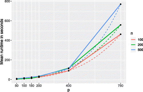
Fig. 2 A typical trajectory of the objective for selecting α for Model 1 $(n=200,p=100,c=0.2)$ in the simulation study in Section 5 (left). The objective in (9) as a function of subset size $n/2\le h\le n$, corresponding to the setting on the left and $\alpha \approx 0.6$. A sudden increase around h = 160, caused by the first outliers being included in the subset.

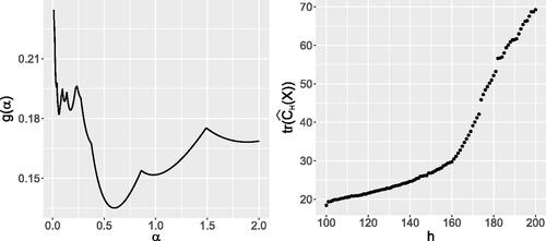
Fig. 3 Left to right, samples from Model 1,2, and 3. Solid curves represent the main processes, while the dashed ones indicate the outliers. The contamination rate is c = 0.1, sample size n = 200, and p = 100 time points.

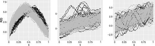
Fig. 4 Left to right: heatmaps of the covariance based on the MRCT estimator, the spatial sign covariance matrix, and the true (theoretical) covariance for n = 200 observations on p = 500 time points for Model 3 with a contamination rate of 20%.

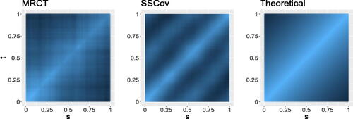
Fig. 5 ISE on a log-scale (top) and COS ${}_{1:5}$ (bottom). The estimates of covariance are based on identified regular observations for $n=200,p=100,500$, and c = 0.2. A solid horizontal line indicates the mean ISE for the sample covariance based on known regular observations as a reference.

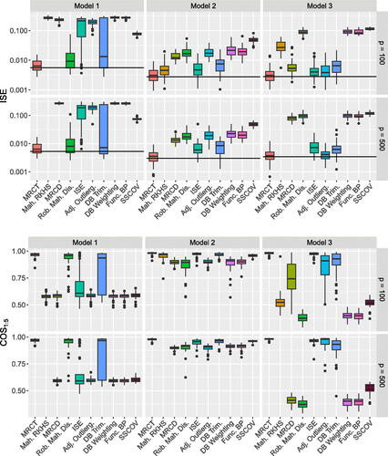
Fig. 6 SST of the Niño 1 + 2 region in the Pacific Ocean. Smoothened regular observations are depicted in gray, while outliers are represented by colored markers. The black dots in the right figure indicate the specific points in time when El Niño events were detected solely using past information, excluding 1982–1984 for the lack of past information.

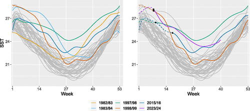
Fig. 7 Left: Spectrum of different glass vessel types. Right: Robust α-Mahalanobis distance on a log-scale. The horizontal line indicates the theoretical cutoff value.

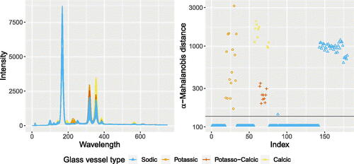
Table 1 True positive and true negative rates for different methods as well as the number of observations considered outlying within the each group.

Method	TPR	TNR	Observations considered outlying
			reg. Sodic	irreg. Sodic	Potassic	Potasso-Calcic	Calcic
Func. BP	1	0	107	38	15	10	10
Rob. Mah. Dis.	0	1	0	0	0	0	0
ISE	0.95	0.80	21	38	11	10	10
DB Trim.	0.50	0.99	1	5	14	8	10
DB Weighting	0.01	1	0	1	0	0	0
MRCT	1	0.99	1	38	15	10	10