Volumetric hyperthermia delivery using the ExAblate Body MR-guided focused ultrasound system

Figures & data

Figure 1. (a) Top view of the ExAblate body transducer and phase distribution of the transducer for the sector-vortex mode 4 at the geometrical focal depth. (b) The concept of mechanical transducer scanning used in this study.

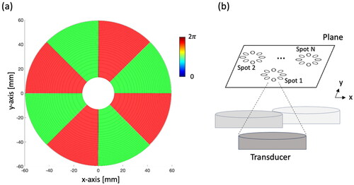
Figure 2. Illustration of the sequential sonication process for multiple heating spots. A series of MR images (N_img) is acquired during sonication, with the number of N_img contingent on the sonication duration (T_s). Notably, a time delay arises between the sonication of each spot due to the transducer movement time (T_mov).

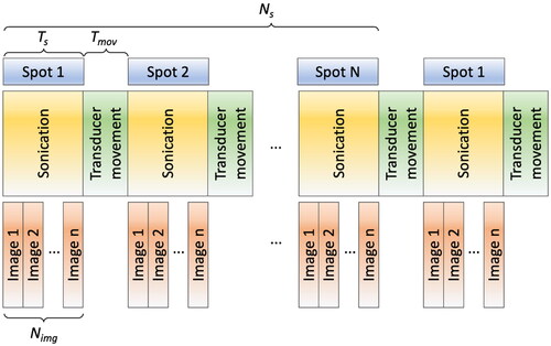
Table 1. The acoustic and thermal properties of the tissue-mimicking phantom were used for the simulation [19, 29] to simulate the perfused tissue, a perfusion rate of 3 kg/m³/s was used throughout the simulation.

Acoustic and thermal properties	Values
Center frequency	1 MHz
Initial temperature	18 °C
Acoustic absorption coefficient	5.8 Np/m/MHz
Speed of sound	1538 m/s
Tissue density	1000 kg/m^3
Heat capacity of phantom	3400 J/°C /kg
Heat capacity of blood	3617 J/°C /kg
Thermal conductivity	0.5 W/m/°C
Perfusion rate	3 kg/m^3/s

Table 2. Hyperthermia control and analysis parameters.

	Simulation	Experiment
Type of feed-back controller	binary feedback control	proportional feedback control
ROI (target area)	20 × 20 × 20 mm^3	(circular) a diameter of 10.9 mm
Field of view	60 × 60 × 130 mm^3	280 × 280 × 3 mm^3
Matrix	160 × 160 × 294	256 × 256
Image update rate	100 ms	3.3 s

Figure 3. Block diagram of temperature feedback control for hyperthermia within the ExAblate Body system. MR temperature images are acquired and visualized on the control computer and used to monitor the temperature throughout the target and within an ROI, which is applied for temperature feedback-based power control through pulse width modulation, thereby facilitating hyperthermia control during MRI scanning.

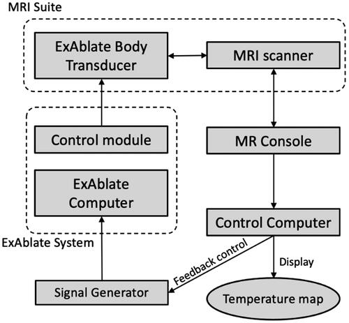
Figure 4. Three different heating patterns and the corresponding temperature distributions for (a) 2, (b) 3, and (c) 4 spots with the distance D_s= 12 mm, sonication time T_s =19 s, and transducer movement time T_mov =12 s. The mask image is generated based on an intensity exceeding 70% of the normalized acoustic intensity. The vortex beam mode 4 is utilized to sonicate each spot, creating multiple foci for large-volume heating. At the end of the thermal simulation, the temperature distributions within the phantom, featuring a simulated perfusion of 3 kg/m³/s, are presented on the X-Y plane and Y-Z plane. The magenta, black, and blue solid lines represent T10, T50, and T90 values, respectively. The green dashed box indicates the ROI to measure T10, T50, and T90 values.

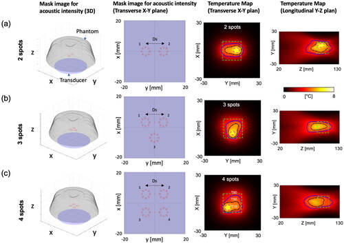
Figure 5. Simulated time-dependent profile in a tissue-mimicking phantom with a simulated perfusion of 3 kg/m³/s within an ROI (20 × 20 × 20 mm³ at the center). The sonication time T_s =19 s and transducer movement time T_mov =12 s are employed. The relative change in temperature is used for the Y-axis scale in the plots. Increasing D_s and the number of spots leads to greater fluctuations in temperature during scanning. This also extends the duration required to reach a target temperature increase of 8 °C.

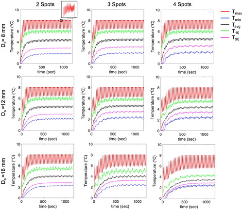
Figure 6. (a) Average values of T10, T50, T90, and difference between T10 and T90. (b) Temperature ripple in Tmax. (c, d) Average values of T10 volume and T50 volume between 10 min and 20 min. Increasing D_s results in reduced average values of T10 and T50 and increased heating volumes and temperature ripple. However, this effect is less pronounced for 2 spots.

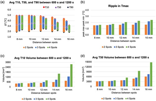
Figure 7. The trend matrix illustrates the relationship between sonication duration (T_s) and transducer movement time (T_mov), characterizing parameter effects on average T10 (a), T50 (b), T90 (c), temperature ripple ([°C], d), and average volume (mm³) for T10 (e) and T50 (f) with the number of spots fixed at 4 and the distance (D_s) set to 12 mm. Average values were computed between 10 to 20 min.

Figure 8. (a) Average temperature map at the focal plane (X-Y plane) for the last 200 s of the simulation, (b-c) a cumulative thermal dose map of CEM and CEMT90 at the focal plane, and (d-e) plots illustrating the maximum peak of CEM based on the distance between spots and transducer movement time. The sonication time is 19 s, and the transducer movement time is 12 s. The green dashed box indicates the targeted ROI to measure T10, T50, and T90 values.

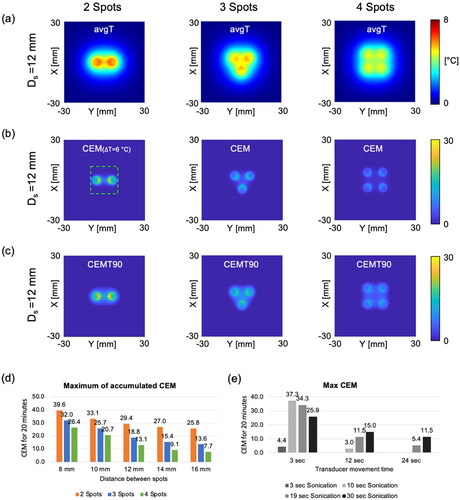
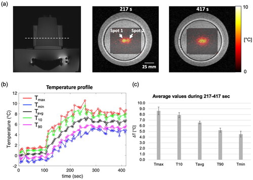
Figure 9. The results of hyperthermia heating on a tissue-mimicking phantom. (a) MR temperature maps overlaid on the corresponding magnitude image at the point when the temperature reached the target temperature and at the end of the experiment. The white-dashed line shows the acquired slice during the experiment. (b) Time-dependent profile of the temperature within a circular ROI with a diameter of 10 pixels (10.9 mm) at the center of the heated region. (c) Average values of Tmax, T10, Tavg, T90 and Tmin during steady-state time interval of 217–417.

Kim K, Zubair M, Adams M, et al. Sonication strategies toward volumetric ultrasound hyperthermia treatment using the ExAblate body MRgFUS system. Int J Hyperthermia. 2021;38(1):1590–1600. doi: 10.1080/02656736.2021.1998658.

 PubMed Web of Science ®Google Scholar

Hasgall PA, Di Gennaro F, Baumgartner C, et al. IT’IS database for thermal and electromagnetic parameters of biological tissues version 4.0. 2018. doi: 10.13099/VIP21000-04-0.

 Google Scholar

Data availability statement

The simulation source codes and/or datasets used in this study are available from the corresponding author upon reasonable request.