Integrated simulation and control environment for the development and safe start-up of cable driven parallel robots

Figures & data

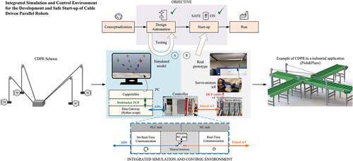
Figure 1. Under-constrained CDPR schematic view.

Figure 2. Closed-loop kinematics model of CDPR.

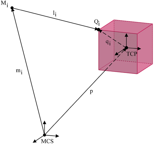
Table 1. Geometrical parameters of the CDPR.

Parameter	$B_l$	$B_w$	$B_h$	$T_l$	$T_w$	$T_h$
Value [mm]	890	1520	1450	58	103	0

Figure 3. Architecture of the proposed environment.

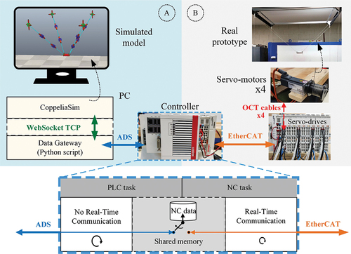
Figure 4. Under-constrained CDPR model in CoppeliaSim. a) tree of components. (b) 3D view.

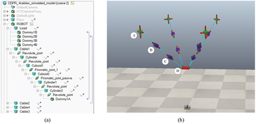
Figure 5. Mechanical and electronics elements of the CDPR prototype.

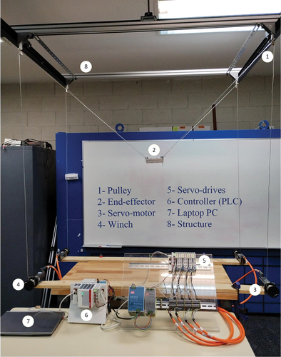
Figure 6. Three-dimensional pick & place trajectory for testing.

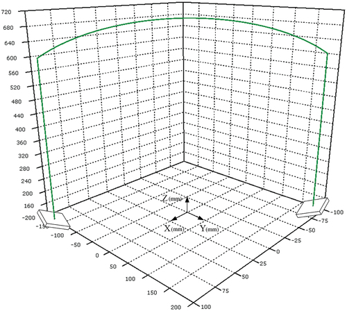
Table 2. Direct kinematic solution of an arbitrary point on the trajectory.

Method Pos	1- Spheres	2- Newton-Raphson	3- Built-in library
X	99.99992488	99.99994526	99.99993776
Y	−174.9999118	−174.999993	−175.0000312
Z	302.8803513	302.8803597	302.880296

Table 3. Comparison of computing time of direct kinematic methods to obtain a new solution.

N	Method	Average [us]	Minimum [us]	Maximum [us]	Number of program cycles to obtain a new solution
1	Spheres	17.52	17	19	1
2	Newton Raphson	32.31	17	41	1
3	Built-in library	18.28	17	20	4

Figure 7. Reaction time difference between the position of the simulated and prototype axes with respect to the target position. a) simulated axis 1 and b) prototype axis 1 at slow speed. c) simulated axis 1 and d) prototype axis 1 at high speed.

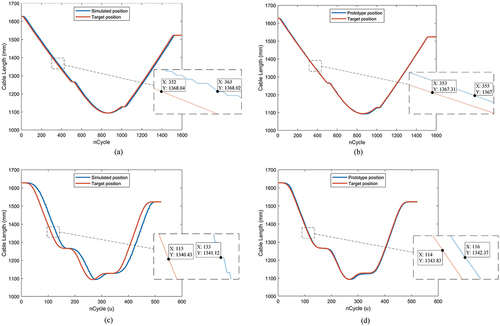
Figure 8. Trajectories of the prototype, simulator, and target at two different speeds. Subfigures (a–c) show trajectories at 100 mm/s, and (d–f) at 500 mm/s, across X-Z, Y-Z, and X-Y planes, respectively.

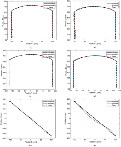
Table 4. Absolute error metrics during trajectory execution.

Phase/Segment	Parameters	Speed
		100 mm/s		500 mm/s
		Simulated	Prototype	Simulated	Prototype
Straight upwards	Average [mm]	0.712	2.364	5.148	6.447
	Standard deviation [mm]	0.403	1.253	3.161	3.815
	Max [mm]	3.085	6.485	14.080	13.225
	Min [mm]	0.028	0.004	0.004	0.008
Displacement	Average [mm]	1.521	2.996	8.087	8.517
	Standard deviation [mm]	0.923	1.692	4.898	2.787
	Max [mm]	7.392	6.865	18.596	14.579
	Min [mm]	0.000	0.152	0.002	3.940
Straight downwards	Average [mm]	0.730	1.312	4.788	4.865
	Standard deviation [mm]	0.468	0.593	3.336	2.708
	Max [mm]	2.862	3.800	13.181	8.219
	Min [mm]	0.000	0.156	0.000	0.385
Complete	Average [mm]	0.979	2.200	5.888	6.504
	Standard deviation [mm]	0.737	1.431	4.065	3.480
	Max [mm]	7.392	6.865	18.596	14.579
	Min [mm]	0.000	0.004	0.000	0.008

Table 5. Mean relative position error during trajectory execution.

Velocity [mm/s]	Mean Relative Position Error [%]
	Simulated	Prototype	Error difference
100	0.19	0.46	0.27
500	1.27	1.42	0.15