
Figures & data
Figure 1. Endemic case in the long run (with ). Left to right
,
,
.
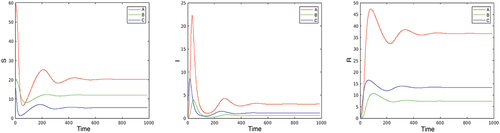
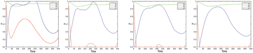
Figure 2. Evolution of (with
) for values of
(left to right).
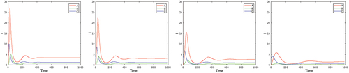
Figure 3. Optimization with respect to both and
in the benchmark case. The first two plots present the optimal controls
and
, the second three plots give the corresponding
,
, and
.
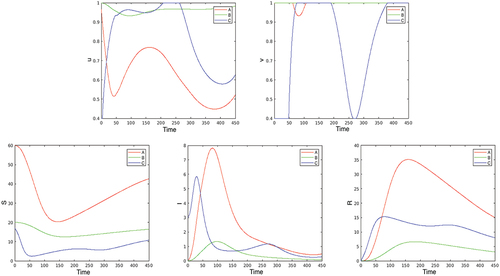
Figure 4. Optimal control for time horizon
, cut at
.
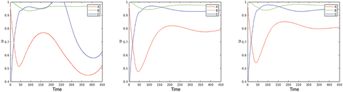
Figure 5. Infected population in the optimal solution for values of (first line), total number of deaths (second line left), and total “control energy”
(second line right)—called “discomfort” on the plot—on
as functions of
.
![Figure 5. Infected population in the optimal solution for values of α=0.2,0.3,0.4,0.5 (first line), total number of deaths (second line left), and total “control energy” E (second line right)—called “discomfort” on the plot—on [0,T] as functions of α.](/cms/asset/8b8220f4-212e-45e7-88c5-b95b4268962b/nmcm_a_2341693_f0005_oc.jpg)
Figure 6. Total number of deaths (left plot) and total social disutility (right plot) in the optimal solution for multiplier of the contact rates varying between 0.2 and 0.8.
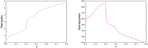
Figure 7. Optimal controls for values of discount
.
Data availability statement
All data supporting the findings of this study are available within the paper.