Predicting the impacts of clearing on vegetation communities: a model-based approach for identifying conservation priorities in Queensland, Australia

Figures & data

Figure 1. Map of the bioregions for this analysis. Areas that have been cleared in the last 30 years are shown in red (as defined by the Statewide Land and Trees Study (SLATS, Department of Science 1988-2016)). Protected areas as of 2019 are shown in green.

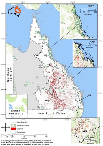
Table 1. Description of each independent predictor variable, the logic behind its inclusion, the data source, year published, and the data type. Datasets by the Queensland Department of Environment and Science, Department of Agriculture and Fisheries, or Department of Natural Resources and Mines were retrieved from http://qldspatial.information.qld.gov.au/catalogue/custom/index.page. We created Rainfall and Temperature data using ANUCLIM http://fennerschool.anu.edu.au/research/products/anuclim-vrsn-61.

Predictor variables	Rationale	Data source	Data year	Data type
Distance to built-up areas	There are higher costs associated with clearing lands that are further from current urban areas (Chomitz and Gray 1999)	Built-up areas: Department of Environment and Science	2014	Continuous
Distance to major roads	Roads facilitate access and are a known correlate to clearing (Chomitz and Gray 1999).	State-controlled roads	2017	Continuous
Distance to watercourses	Increased access to surface water increases the likelihood of land development for agricultural or grazing purposes.	Watercourses: Department of Environment and Science	2014	Continuous
Grass biomass	Lands with higher pasture production are more likely to be cleared for grazing and less likely to be protected due to higher production value.	Agricultural land audit: Department of Agriculture and Fisheries	2014	Continuous
Rainfall	Land arability is a combination of climatic variables which may lead to competition between protection and production (Nori et al. 2013)	ANUCLIM	2017	Continuous
Slope	Flatland (low per cent slope) is easier to clear (Wilson et al. 2005)	Digital elevation model: Department of Natural Resources and Mines	2013	Continuous
Temperature	Land arability is a combination of climatic variables which may lead to competition between protection and production (Nori et al. 2013)	ANUCLIM	2017	Continuous

Figure 2. Schematic representation of the modelling procedure. Predictor variables listed in Table 1 were rasterised to a 250*250 m resolution and then stacked into a single dataset per bioregion. We used a generalised estimating equation to predict deforestation probability.

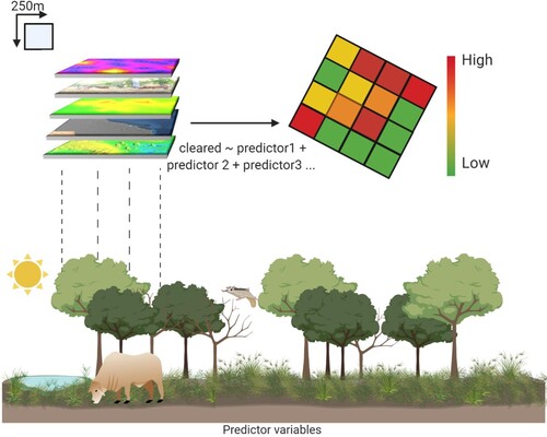
Table 2. A description of the variables included in the final model (p < 0.05) for each bioregion. ‘Built’ refers to Euclidean distance to built-up areas, ‘graze’ refers to grass biomass, ‘rain’ refers to average annual rainfall, ‘roads’ refers to Euclidean distance to State-controlled roads, ‘slope’ refers to slope in per cent rise, ‘temp’ refers to yearly average temperature, ‘wc’ refers to Euclidean distance to major watercourses. The third column shows the mean (M) of simulated Pearson’s Chi-Squared goodness-of-fit values. Chi-square tests whether or not the observed data are consistent with the values imputed from the models (Alsadik 2019). ^{^} indicates that there is no significant difference between the predicted and observed clearing data and the models have performed well. The final column is the mean (M) confidence interval (upper and lower 95 per cent of values) for each bioregion (see methods: model confidence).

Bioregion	List of covariates	M.Chi – Square	M.df	M.pvalue	M. Confidence intervals
Brigalow Belt	Built, rain, roads, slope, temp, wc	97855	97853	0.4980^^	0.103 ± 5.27*10^−5
Cape York	Graze, rain, slope, temp wc	96995	96994	0.4919^^	3.40*10^−3 ± 7.35*10^−6
Central Queensland Coast	Graze, rain, roads, slope, temp, wc	78567	78573	0.5083^^	3.697*10^–2± 1.53*10^−4
Desert Uplands	Graze, rain, roads, slope, temp, wc	95021	95017	0.4961^^	0.0910 ± 1.96*10^−4
Einasleigh Uplands	Built, graze, rain, roads, slope, temp, wc	98645	98646	0.4993^^	1.016*10^–2± 8.57*10^−6
Mulga Lands	Graze, rain, slope, temp, wc	98176	98174	0.4976^^	0.0990 ± 1.35*10^−4
New England Tablelands	Built, roads, slope, temp, wc	66508	66498	0.4918^^	0.0714 ± 1.71*10^−4
Southeast Queensland	Built, graze, roads, rain, slope, temp, wc	94595	94586	0.4921^^	0.0512 ± 7.85*10^−5
Wet Tropics	Built, graze, rain, roads, slope, temp, wc	83461	83466	0.5006^^	0.0224 ± 1.21*10^−4

Figure 3. Map of the likelihood that a pixel will be cleared given the relevant biophysical characteristics of the pixel. The predicted values for each bioregion are shown in a combined raster format ‘predicted values.’BB = Brigalow Belt, CY = Cape York, CQC = Central Queensland Coast, DU = Desert Uplands, EU = Einasleigh Uplands, Mulga = Mulga Lands, NET = New England Tablelands, SEQ = Southeast Queensland, WET = Wet Tropics.

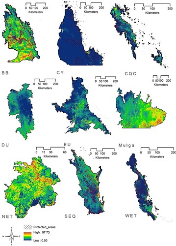
Table 3. Summary table of the number of regional ecosystems affected in each bioregion per scenario. Number is the number of regional ecosystems affected under each of the scenarios. 1 status change is the number of regional ecosystems that will change status once and 2 status changes are those that will change status twice (i.e. from Least Concern to to Endangered) under each scenario.

	Low Scenario			Moderate Scenario			High Scenario
Bioregion	Number	1 status change	2 status changes	Number	1 status change	2 status changes	Number	1 status change	2 status changes
Brigalow Belt	114	2	–	157	30	6	166	74	27
Cape York	1	1	–	20	–	–	66	1	–
Central Queensland Coast	8	3	–	41	2	–	65	7	–
Desert Uplands	69	–	–	74	8	–	75	15	3
Einasleigh Uplands	19	1	–	51	–	–	78	–	–
Mulga Lands	40	7	–	64	29	9	64	45	31
New England Tablelands	5	–	–	13	1	–	22	4	2
Southeast Queensland	12	12	2	126	17	4	152	12	9
Total	268	26	2	546	87	19	688	158	72

Department of Science, Information Technology and Innovation. 1988-2016. State Wide Land And Trees Study (SLATS). Dutton park, Queensland 4102: Queensland Government.

 Google Scholar

Chomitz, Kenneth, and David A Gray. 1999. Roads, Lands, Markets, and Deforestation: A Spatial Model of Land use in Belize. Routledge: The World Bank.

 Google Scholar

Nori, Javier, Julián N. Lescano, Patricia Illoldi-Rangel, Nicolás Frutos, Mario R. Cabrera, and Gerardo C. Leynaud. 2013. “The Conflict Between Agricultural Expansion and Priority Conservation Areas: Making the Right Decisions Before it is Too Late.” Biological Conservation 159: 507–513. https://doi.org/10.1016/j.biocon.2012.11.020.

 Web of Science ®Google Scholar

Wilson, Kerrie, Robert L Pressey, Adrian Newton, Mark Burgman, Hugh Possingham, and Chris Weston. 2005. “Measuring and Incorporating Vulnerability Into Conservation Planning.” Environmental Management 35 (5): 527–543. https://doi.org/10.1007/s00267-004-0095-9

 PubMed Web of Science ®Google Scholar

Alsadik, Bashar. 2019. “Chapter 12 - Postanalysis in Adjustment Computations.” In Adjustment Models in 3D Geomatics and Computational Geophysics, edited by Bashar Alsadik, 345–385. Amsterdam, Netherlands: Elsevier.

 Google Scholar