Coastal ocean forecasting on the GPU using a two-dimensional finite-volume scheme

Figures & data

Fig. 1. a) The relationship between the physical variables h, H, η, and hu used in the shallow-water equations, here shown in one dimension. b) The ocean state is discretised in terms of cell average values, whereas the bathymetry is defined at the cell intersections. c) We find the slopes of the ocean state within each cell. d) The flux between the cells is found from two one-sided point values at each interface, as seen from the two adjacent cells.

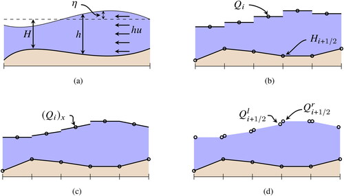
Fig. 2. Desingularization of the quantity $u=h/hu$ using existing and our proposed method with $\kappa =1.0·{10}^{-11}$ for all cases. We compute the value of hu / h using the different approaches for u = 1 and different values of h. Notice how the single precision floating-point errors are clearly visible for $u_1^{*},$ that $u_2^{*}$ has a distinct kink, and that $u_3^{*}$ significantly underestimates the true magnitude of u.

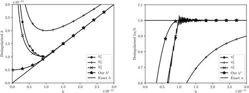
Fig. 3. Planetary Rossby waves generated by a beta plane model for the Coriolis force and with different directions for north. The simulations are initialised by a rotating bump in the middle of the domain, which develops into Rossby waves that propagates westwards with wave energy slowly propagating eastwards. The different figures show that we get the same Rossby waves for arbitrary orientation of our domain. Axes are given in 1000 km, and the colormap shows η in m.

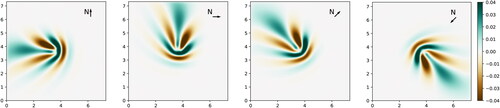
Fig. 4. Reconstruction of the bathymetry at intersection points. Starting with the initial bathymetry H_m defined at cell midpoints (upper left), we compute the H_i values at intersections (upper right). The lower-left figure shows the convergence of our reconstruction algorithm, and the reconstructed bathymetry is plotted together with the original in the lower-right figure. The top two figures have axes units in number of cells, and the x-axis in the bottom right is similarly in number of cells. The y-axis in the bottom right figure shows the depth. Notice that small features such as islands can disappear in the top right figure, but that the bathymetry does not appear to suffer from smoothing caused by the interpolation procedure.

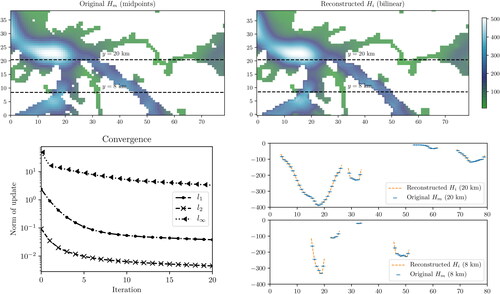
Fig. 5. Widening of narrow straits, in which the land mask is eroded using binary erosion. The left figure shows particle velocities in the Tjeldsund strait in Lofoten/Vesterålen between the main land and Hinnøya (the bathymetry is shown in Fig. 4). Left shows the NorKyst-800 reference, centre shows original (reconstructed) bathymetry, and the right figure shows the result with one grid cell land erosion. The strait width and geometry limits the amount of water passing through it in the original bathymetry, but by eroding one cell of the land mask the amount of water is much closer to the reference. The axis units are in number of grid cells.

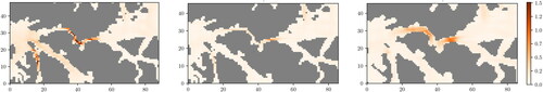
Fig. 6. Convergence plot of our numerical scheme. The numerical case has a water disturbance consisting of a cosine bump at the centre of the domain, and the bathymetry consists of the smooth Matlab peaks function. The Coriolis force varies spatially across the domain according to variations in latitude and direction towards north. The left figure shows the self convergence of the numerical error compared to the reference solution with 1024² cells. To the right we show the bathymetry with the sea-surface level initially (top) and at the end of the simulation (bottom). The horizontal axis are in kilometres, and the vertical axis is in metres. Notice that the height of the bump is slightly reduced in the lower figure (smaller white area).

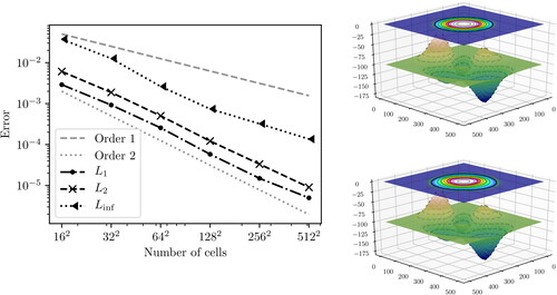
Table 1. Error of computed solutions at different resolutions and numerical reduction order for each refinement. The time step is fixed throughout these simulations.

Resolution	$\Delta t$	L1	Order	L2	Order	$L_{\text{inf}}$	Order
16^2	1600/16	0.002898	–	0.006072	–	0.037367	–
32^2	1600/32	0.000923	1.65	0.001877	1.69	0.012651	1.56
64^2	1600/64	0.000256	1.85	0.000502	1.90	0.002621	2.27
128^2	1600/128	0.000058	2.14	0.000122	2.04	0.000741	1.82
256^2	1600/256	0.000015	1.96	0.000033	1.87	0.000322	1.20
512^2	1600/512	0.000005	1.58	0.000009	1.89	0.000136	1.25

Fig. 7. Weak scaling of our simulator. For small domain sizes, the runtime is dominated by overheads, but for domain sizes larger than approximately 512 × 512, we see that the computational time scales with the number of cells. For each doubling of our domain, we perform approximately eight times as many operations (four times as many cells, and twice the number of time steps).

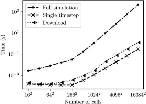
Table 2. Performance for our simulator. The simulation time is approximately eight times larger when we double the resolution. This is because we have four times as many cells and twice as many timesteps to reach the same end time. The download increases by a factor four, which is to be expected as we transfer four times as many data elements.

Resolution	Simulation time	Factor	Download time	Factor
512^2	0.169710	–	0.000929	–
1024^2	1.170814	6.9	0.002773	3.0
2048^2	9.133564	7.8	0.019642	7.1
4096^2	72.832028	8.0	0.077541	3.9
8192^2	582.599290	8.0	0.305405	3.9
16384^2	4695.904546	8.0	1.218880	4.0

Fig. 8. The domain covered by the NorKyst-800 model showing the equilibrium depth off shore. The location of Case 1 in the Norwegian Sea (yellow rectangle), Case 2 around the Lofoten archipelago (red rectangle), and Case 3 (beige rectangle) within the NorKyst-800 model domain, with red stars marking the locations for sea-level predictions. The values on the x- and y-axes are given in km, and the latitude-longitude grid shows how the direction towards north changes throughout the domain.

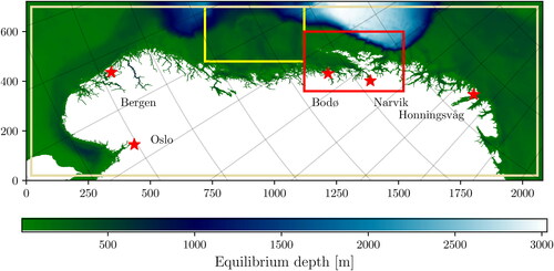
Fig. 9. Case 1 of the Norwegian Sea after 23 hours, comparing the reference solution from NorKyst-800 with our simulations using three different grid resolutions. All simulations obtain sea-surface level (left) similar to the reference solution, meaning that the boundary conditions allow the tides to correctly enter and exit our domain. From the particle velocities (right), we see that only the high-resolution model is able to maintain sharp features, whereas the low-resolution simulation has strong signs of grid effects. The values on the x- and y-axes are in km relative to the location in the complete domain.

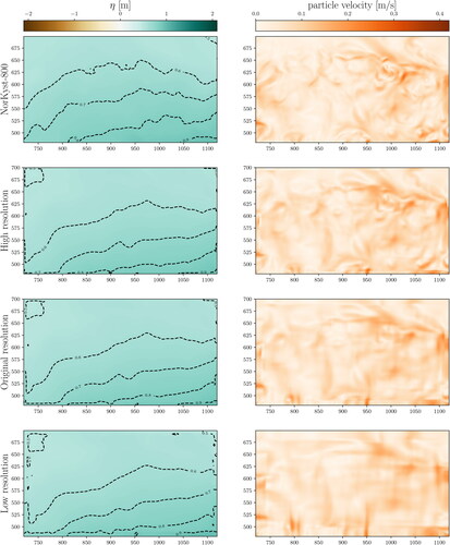
Fig. 10. Case 2 around the Lofoten archipelago after 23 hours, comparing the reference solution from NorKyst-800 with our simulations using three different grid resolutions. The values on the x- and y-axes are in km relative to the location in the complete domain. Our sea-surface levels (left column) are similar but slightly higher within Vestfjorden compared to the reference solution. From the particle velocities (right), we see that we get stronger currents than the reference. The level of details in our simulations are stronger with higher grid resolution, whereas the low-resolution simulation blurs the structures and are influenced by grid effects.

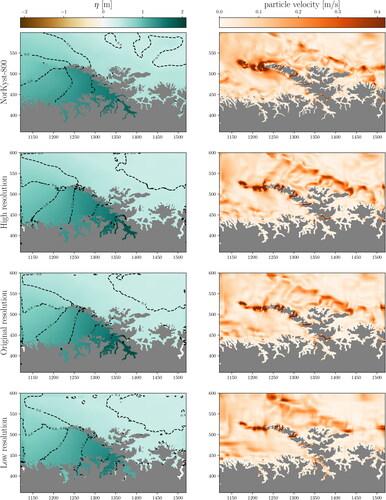
Fig. 11. Simulation result for Case 3 containing almost the complete domain used by NorKyst-800 after 23 hours. The top row shows the reference solution from NorKyst-800, followed by our simulation results using three different grid resolutions below. The values on the x- and y-axes are in km relative to the location in the complete domain. The sea-surface levels (left) show how the tide varies along the coast, with low tide in the Oslofjord (lower left corner), high tide in the middle of the domain, and low tide again towards the border with Russia (lower right corner). Our results are consistent with the reference solution for all grid resolutions. The particle velocities (right column) are qualitatively similar for the reference solution (NorKyst-800), and our simulations with high and original resolution. Even at this scale, it is apparent that the low resolution grid smears the features in the ocean currents.

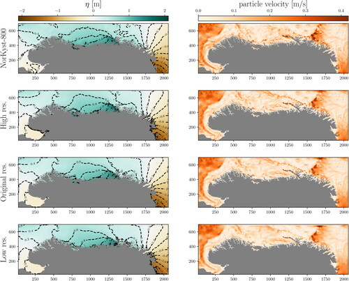
Table 3. Timing results different resolutions of running the complete Norwegian coast (Case 3), excluding initialisation, with the original, high and low resolution on different computer types.

Resolution	Num cells	Average $\Delta t$	Laptop GeForce 840M Maxwell (2014)	Desktop GeForce GTX780 Kepler (2013)	Server Tesla P100 Pascal (2016)
Low	541 875	1.85 s	9m 22 s	1 m 29 s	47 s
Original	2 167 500	0.92 s	53m 49 s	10 m 42 s	3 m 13 s
High	8 670 000	0.46 s	6h 10 m 09 s	1 h 23 m 22 s	23 m 21 s

Table 4. Breakdown of run time for simulating 23 hours of the complete Norwegian coast (Case 3) on the desktop with a GeForce GTX780 GPU. The column with time spent writing to disc includes downloading from the GPU and all over overhead required for this operation.

Resolution	Initialisation	Simulation 1 hour	Write one time step to disc (fraction of simulation time)
Low	15.6 s	3.4 s (85.3%)	0.5 s (14.7%)
Original	11.8 s	25.9 s (92.3%)	2.0 s (7.7%)
High	18.3 s	209.5 s (96.2%)	8.0 s (3.8%)

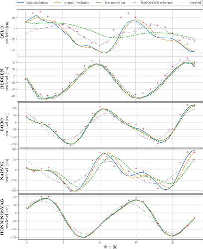
Fig. 12. Tidal predictions, reference NorKyst-800 results, and official gauge measurements every five minutes at selected locations generated by the simulations discussed in Case 3. All grid resolutions capture the tide as predicted by NorKyst-800 with only minor discrepancies at coastal locations, such as Bergen, Bodø and Honningsvåg. The grid resolution comes much more into play deep inside the fjords, such as at Oslo and Narvik. Here, the low-resolutions grid no longer manages to represent the bathymetry well enough for the tide to enter the fjord correctly (especially in the very narrow Oslo fjord), but we still get fair results with the high-resolution grid. The weakly dotted line is actual observed sea-surface level at the respective locations in the time range of the forecast. It should be noted that official tidal forecasts have additional physical terms, which is the main reason why the NorKyst-800 is off.