Investigating the impact of vaccine hesitancy on an emerging infectious disease: a mathematical and numerical analysis

Figures & data

Figure 1. Schematic diagram for the dynamics of an emerging disease in the presence of vaccination, with three infected classes of increasing symptom severity.

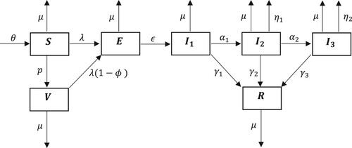
Table 1. Definitions of parameters used in the model.

Parameter	Definition
μ	Natural mortality rate
θ	Recruitment rate
p	Vaccination coverage rate
ϕ	Vaccine efficacy
ϵ	Incubation rate
${\alpha }_1$	Rate of progression from mild symptoms to moderate symptoms
${\alpha }_2$	Rate of progression from moderate symptoms to severe symptoms
${\text{β}}_1$	Transmission coefficient for individuals infected with mild symptoms
${\text{β}}_2$	Transmission coefficient for individuals infected with moderate symptoms
${\text{β}}_3$	Transmission coefficient for individuals infected with severe symptoms
${\gamma }_1$	Recovery rate for individuals infected with mild symptoms
${\gamma }_2$	Recovery rate for individuals infected with moderate symptoms
${\gamma }_3$	Recovery rate for individuals infected with severe symptoms
${\eta }_1$	Diseased-induced death rate for individuals infected with moderate symptoms
${\eta }_2$	Diseased-induced death rate for individuals infected with severe symptoms

Table 2. Parameter values used for numerical simulations.

Parameter	Value	Units	Source/s
μ	2.7e−5	$\frac{1}{\mathrm{d}\mathrm{a}\mathrm{y}}$	Assumed *
θ	0.277	$\frac{\mathrm{i}\mathrm{n}\mathrm{d}\mathrm{i}\mathrm{v}\mathrm{i}\mathrm{d}\mathrm{u}\mathrm{a}\mathrm{l}}{\mathrm{d}\mathrm{a}\mathrm{y}}$	Set to $\mu N\left(0\right)$
p	0.05	$\frac{1}{\mathrm{d}\mathrm{a}\mathrm{y}}$	Assumed ^†
ϕ	95%	$\mathrm{d}\mathrm{i}\mathrm{m}\mathrm{e}\mathrm{n}\mathrm{s}\mathrm{i}\mathrm{o}\mathrm{n}\mathrm{l}\mathrm{e}\mathrm{s}\mathrm{s}$	[16,17]
ϵ	0.084	$\frac{1}{\mathrm{d}\mathrm{a}\mathrm{y}}$	[16,18–20]
${\alpha }_1$	0.06	$\frac{1}{\mathrm{d}\mathrm{a}\mathrm{y}}$	Assumed ^‡
${\alpha }_2$	0.01	$\frac{1}{\mathrm{d}\mathrm{a}\mathrm{y}}$	Assumed ^§
${\text{β}}_1$	4e−4	$\frac{1}{\mathrm{i}\mathrm{n}\mathrm{d}\mathrm{i}\mathrm{v}\mathrm{i}\mathrm{d}\mathrm{u}\mathrm{a}\mathrm{l}\times \mathrm{d}\mathrm{a}\mathrm{y}}$	[16,19,20]
${\text{β}}_2$	3e−4	$\frac{1}{\mathrm{i}\mathrm{n}\mathrm{d}\mathrm{i}\mathrm{v}\mathrm{i}\mathrm{d}\mathrm{u}\mathrm{a}\mathrm{l}\times \mathrm{d}\mathrm{a}\mathrm{y}}$	[16,19]
${\text{β}}_3$	2e−4	$\frac{1}{\mathrm{i}\mathrm{n}\mathrm{d}\mathrm{i}\mathrm{v}\mathrm{i}\mathrm{d}\mathrm{u}\mathrm{a}\mathrm{l}\times \mathrm{d}\mathrm{a}\mathrm{y}}$	[16,19,20]
${\gamma }_1$	0.2	$\frac{1}{\mathrm{d}\mathrm{a}\mathrm{y}}$	[16,19,20]
${\gamma }_2$	0.1	$\frac{1}{\mathrm{d}\mathrm{a}\mathrm{y}}$	[16,19]
${\gamma }_3$	0.08	$\frac{1}{\mathrm{d}\mathrm{a}\mathrm{y}}$	[16,19,20]
${\eta }_1$	0.009	$\frac{1}{\mathrm{d}\mathrm{a}\mathrm{y}}$	Assumed ^#
${\eta }_2$	0.011	$\frac{1}{\mathrm{d}\mathrm{a}\mathrm{y}}$	[16,21]

Note: Since the study is focused on an emerging respiratory infection, we use parameter values drawn from the literature of COVID-19, which is the most recent respiratory infection to affect the world at a pandemic level.*Since the population used for the simulations is hypothetical, the value for μ was chosen based upon values from the general literature.^†This value was assigned based upon a 5% vaccination coverage rate. ^{‡, §} These values were assumed based on the value of ϵ and the relation $ϵ<{\alpha }_1<{\alpha }_2$. ^# This value was assumed based on the value of ${\eta }_2$ and the relation ${\eta }_1<{\eta }_2$.

Figure 2. The bifurcation diagram for the equilibria of model (1(1) $\begin{array}{rl}& \frac{\mathrm{d}S}{\mathrm{d}t}=\theta -(\mu +p+\lambda )S\\ & \frac{\mathrm{d}V}{\mathrm{d}t}=pS-[\mu +\lambda (1-\varphi \left)\right]V\\ & \frac{\mathrm{d}E}{\mathrm{d}t}=\lambda S+\lambda (1-\varphi )V-(\mu +ϵ)E\\ & \frac{\mathrm{d}{I}_1}{\mathrm{d}t}=ϵE-(\mu +{\alpha }_1+{\gamma }_1)I_1\\ & \frac{\mathrm{d}{I}_2}{\mathrm{d}t}={\alpha }_1{I}_1-(\mu +{\eta }_1+{\alpha }_2+{\gamma }_2)I_2\\ & \frac{\mathrm{d}{I}_3}{\mathrm{d}t}={\alpha }_2{I}_2-(\mu +{\eta }_2+{\gamma }_3)I_3\\ & \frac{\mathrm{d}R}{\mathrm{d}t}={\gamma }_1{I}_1+{\gamma }_2{I}_2+{\gamma }_3{I}_3-\mu R\end{array}$(1) ) with respect to vaccine efficacy $\left(\varphi \right)$. This plot illustrates the sum of infected components of the disease-free equilibrium (horizontal line) and endemic equilibrium (curve), with respect to varying values of ϕ. All other parameters are fixed as in Table 2. Red (dashed) indicates that the steady state is unstable, and blue (solid) indicates it is stable.

Figure 3. A graphical illustration (i.e. tornado plot) of the sensitivity indices of the model parameters. Since the vaccine efficacy (ϕ) has an extremely large negative sensitivity index (see Table 3), we instead use the sensitivity index of the vaccine failure (ζ) for the convenience of understanding the graphical representation.

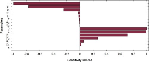
Table 3. Sensitivity indices of the model parameters using differential sensitivity analysis [28].

Parameter (ω)	Sensitivity index ($S_{\omega }$)
ϕ	−18.797
μ	−0.9903
${\gamma }_1$	−0.7686
${\gamma }_2$	−0.2423
${\eta }_1$	−0.0218
${\gamma }_3$	−0.0173
p	−0.0101
${\alpha }_2$	−0.0046
${\eta }_2$	−0.0024
θ	1
ζ *	0.9893
${\text{β}}_1$	0.7114
${\text{β}}_2$	0.2689
${\alpha }_1$	0.0579
${\text{β}}_3$	0.0197
ϵ	0.0003

Note: The parameter values are as in Table 2.*Note that $\zeta =1-\varphi$.

Figure 4. Variation in ${\mathcal{R}}_0$ according to different pairs of parameters. The remaining parameters are fixed as in Table 2. The ranges of parameters were chosen to show the most pertinent model behaviour near the threshold of ${\mathcal{R}}_0=1$. Note that the choice of distinct colours is intended for better illustration of results, and does not mean that ${\mathcal{R}}_0$ has discontinuous jumps. (a) Variation in ${\mathcal{R}}_0$ according to ${\text{β}}_1$ and p. (b) Variation in ${\mathcal{R}}_0$ according to ${\text{β}}_1$ and ϕ. (c) Variation in ${\mathcal{R}}_0$ according to p and ϕ.

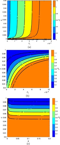
Figure 5. Cumulative number of disease-induced deaths given various values of vaccine efficacy (ϕ) between 0.9 and 1. All other parameters are fixed as in Table 2.

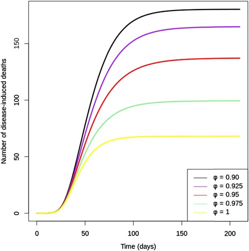
Figure 6. Change in (a) $I_1$, (b) $I_2$, and (c) $I_3$ over time with various levels of vaccine hesitancy (ψ) between 0 and 1, with proportionality constant k = 0.05 and vaccine efficacy $\varphi =0.95$. All other parameters are fixed as in Table 2. Note the different scales for the vertical axes. (a) Infections with mild symptoms over time. (b) Infections with moderate symptoms over time. (c) Infections with severe symptoms over time.

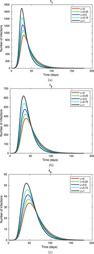
Figure 7. Cumulative number of disease-induced deaths given various values of vaccine hesitancy (ψ) between 0 and 1. Note that k = 0.05 and all other parameters are fixed as in Table 2.

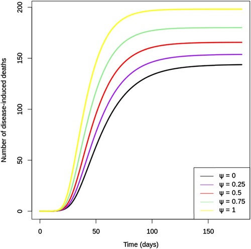
Table 4. The vaccine efficacy required to compensate for different levels of vaccine hesitancy.

Vaccine hesitancy (ψ)	Goal	Requirement on vaccine efficacy (ϕ)
10%	Reduce $I_1^{max}$ by 40%	$\varphi =0.93675$
	Reduce $I_2^{max}$ by 40%	$\varphi =0.96704$
	Reduce $I_3^{max}$ by 40%	$\varphi =0.97928$
25%	Reduce $I_1^{max}$ by 40%	$\varphi =0.97090$
	Reduce $I_2^{max}$ by 40%	$\varphi =0.99276$
	Reduce $I_3^{max}$ by 40%	$\varphi =0.99865$
60%	Reduce $I_1^{max}$ by 40%	Infeasible
		($\varphi =1⟹27.57\mathrm{\%}$ drop in $I_1^{max}$)
	Reduce $I_2^{max}$ by 40%	Infeasible
		($\varphi =1⟹25.85\mathrm{\%}$ drop in $I_3^{max}$)
	Reduce $I_3^{max}$ by 40%	Infeasible
		($\varphi =1⟹25.22\mathrm{\%}$ drop in $I_3^{max}$)

Note: Value of peak infection = $I_i^{max}$. Note that k = 0.05 and all other parameters are fixed as in Table 2.

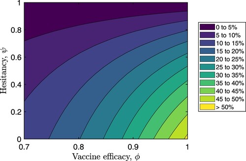
Figure 8. Percentage reductions in the peak of total infection (i.e. the sum $I_1+I_2+I_3$) for varying values of vaccine efficacy (ϕ) and vaccine hesitancy (ψ). All other parameters are fixed as in Table 2.

Centers for Disease Control & Prevention. COVID-19 and your health. Centers for disease control and prevention; 2020 Feb. Available from: https://www.cdc.gov/coronavirus/2019-ncov/your-health/about-covid-19/basics-covid-19.html.

 Google Scholar

E.P. Esteban, L. Almodovar-Abreu. Assessing the impact of vaccination in a COVID-19 compartmental model. Inform Med Unlocked. 2021;27:Article ID 100795. doi: 10.1016/j.imu.2021.100795

 PubMedGoogle Scholar

National Institute of Health. Clinical spectrum of SARS-CoV-2 infection; n.d. Available from: https://www.covid19treatmentguidelines.nih.gov/overview/clinical-spectrum/.

 Google Scholar

T. Šušteršič, A. Blagojević, D. Cvetković, et al. Epidemiological predictive modeling of COVID-19 infection: development, testing, and implementation on the population of the benelux union. Front Public Health 9 (2021), pp. 1–24. doi:10.3389/fpubh.2021.727274.

 Web of Science ®Google Scholar

Johns Hopkins Coronavirus Resource Center. Mortality analyses; n.d. Available from: https://coronavirus.jhu.edu/data/mortality.

 Google Scholar

C.W. Castillo-Garsow, C. Castillo-Chavez, A tour of the basic reproductive number and the next generation of researchers, in An Introduction to Undergraduate Research in Computational and Mathematical Biology, H. Callender Highlander, A. Capaldi, and C. Diaz Eaton, ed., Foundations for Undergraduate Research in Mathematics, Birkhäuser, Cham, 2020. doi:10.1007/978-3-030-33645-5_2

 Google Scholar