Figures & data
Figure 1. Visualization the modes of one-dimensional scaled Legendre basis polynomials corresponding to the 4th-order approximation.
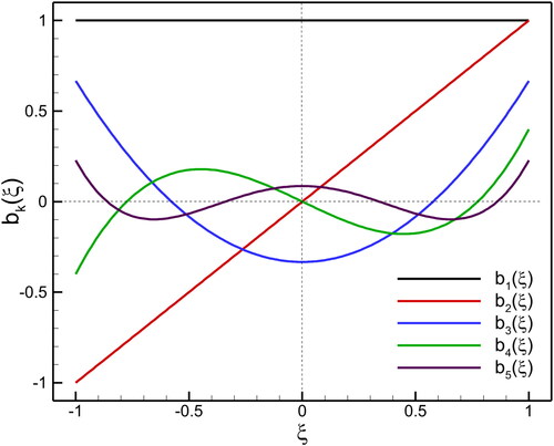
Table 1. Accuracy test of the linear scalar problem.
Figure 2. Validation of numerical solver: comparison of exact and numerical solutions for the calculated quantities (a) density and (b) pressure at in classical Sod shock tube problem.
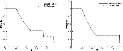
Figure 3. Graphical representation and initial configuration of shock tube problem.
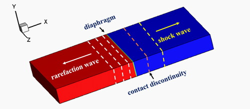
Figure 4. Time evolution of density profiles for G13 (solid line), and G5 equations (dashed line) at Kn
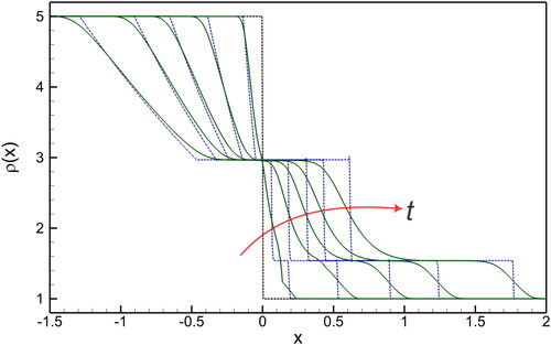
Figure 5. Shock tube problem: Kn number effect on macroscopic quantities (density (), pressure (p), velocity (v), temperature (
), stress (
), and heat flux (q)) in the G5 and G13 systems at
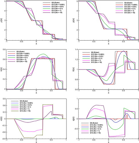
Figure 6. Shock tube problem: Kn number effect on the solutions of normal stress vs heat flux in the G13 system at
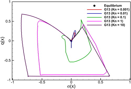
Figure 7. Kn number effect on the spatiotemporal contours for density solution in the G5 and G13 systems. In each sub-figure, horizontal axis denotes the while vertical axis represents the time
![Figure 7. Kn number effect on the spatiotemporal contours for density solution in the G5 and G13 systems. In each sub-figure, horizontal axis denotes the x∈[−4.0,4.0], while vertical axis represents the time t∈[0,1.5].](/cms/asset/39b39cab-c908-42d9-b1d7-47fd1ea35a84/ltty_a_2342947_f0007_c.jpg)
Figure 8. Kn number effect on the spatiotemporal contours for pressure solution in the G5 and G13 systems. In each sub-figure, horizontal axis denotes the while vertical axis represents the time
![Figure 8. Kn number effect on the spatiotemporal contours for pressure solution in the G5 and G13 systems. In each sub-figure, horizontal axis denotes the x∈[−4.0,4.0], while vertical axis represents the time t∈[0,1.5].](/cms/asset/46595db6-272f-47a9-95cf-5918843833d2/ltty_a_2342947_f0008_c.jpg)
Figure 9. Kn number effect on the spatiotemporal contours for heat flux solution in the G5 and G13 systems. In each sub-figure, horizontal axis denotes the while vertical axis represents the time
![Figure 9. Kn number effect on the spatiotemporal contours for heat flux solution in the G5 and G13 systems. In each sub-figure, horizontal axis denotes the x∈[−4.0,4.0], while vertical axis represents the time t∈[0,1.5].](/cms/asset/dade0fbc-7f14-403c-81bb-88f3d36a2177/ltty_a_2342947_f0009_c.jpg)
Figure 10. Kn number effect on the several solutions of the G13 system with different pressure ratios in the hyperbolicity region.
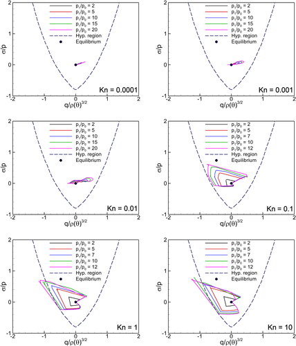
Figure 11. Hyperbolicity boundary and two different initial conditions for G13 system. For pressure ratio of 15, the ellipticity of G13 equations leads to oscillations and break-down of the computation.
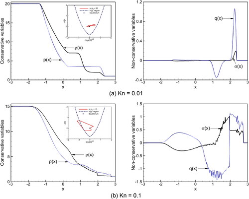
Figure 12. Shock tube problem: profile for pressure ratio vs Kn number.
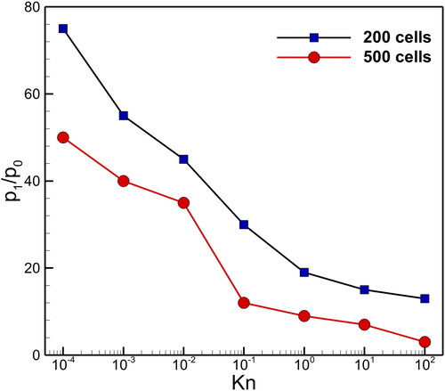
Figure 13. Two shock waves: Kn effects on macroscopic quantities in the G5 and G13 systems at
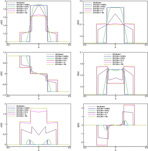
Figure 14. Two shock waves: Kn effects on the solutions of normal stress vs heat flux in the G13 system at
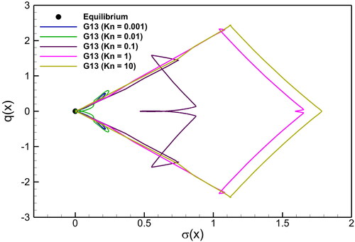
Figure 15. Two rarefaction waves: Kn effect on macroscopic quantities in the G5 and G13 systems at
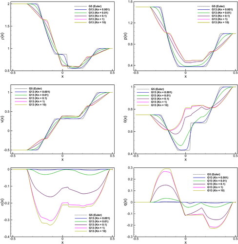
Figure 16. Two rarefaction waves: Kn effects on the solutions of nomral stress vs heat flux in the G13 system at
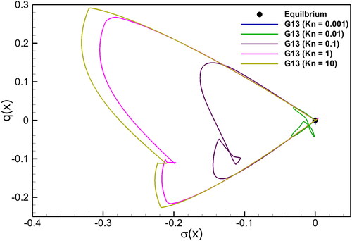
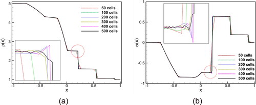
Figure A1. Grid convergence study in shock tube problem at Kn = 1: profiles of (a) density, and (b) heat flux quantities for six different cells.