Tractable Bayesian Inference For An Unidentified Simple Linear Regression Model

Abstract

In this article, I propose a tractable approach to Bayesian inference in a simple linear regression model for which the standard exogeneity assumption does not hold. By specifying a beta prior for the squared correlation between an error term and regressor, I demonstrate that the implied prior for a bias parameter is t-distributed. If the posterior distribution for the identified regression coefficient is normal, this implies that the posterior distribution for the unidentified treatment effect is the convolution of a normal distribution and a t-distribution. This result is closely related to the literatures on unidentified regression models, imperfect instrumental variables, and sensitivity analysis.

Keywords:

• Bayesian statistics
• Identification
• Linear regression
• Omitted variable bias
• Sensitivity analysis
• Unidentified models

1 Introduction

Consider the simple linear regression model, (1) $$Y=\beta X+U,$$(1) in which the regressand Y, the regressor X, and the error term U are mean-zero random variables.

As is well known, this model is identified if $\mathrm{E}[U|X]=0$, which is a sufficient condition for $\mathrm{E}[U]=0$ and $\text{Cov}[X,U]=0$ (Wooldridge 2010, chap. 4). Identification, in this context, means that each unique value of β implies a unique likelihood function. More precisely, there are no pairs β₁ and β₂ that generate likelihood functions $\mathrm{L}$ such that $\mathrm{L}({\beta }_1)=\mathrm{L}({\beta }_2)$. Identified models, in other words, do not suffer from observational equivalence (Wechsler, Izbicki, and Esteves 2013).

If $\mathrm{E}[U|X]\ne 0$, however, a sample of observations on Y and X will not permit simultaneous estimation of β and $\mathrm{E}[U|X]$. In this case, the linear regression model is unidentified. As discussed below, this is because there exist pairs $\left({\beta }_1,\mathrm{E}{[U|X]}_1\right)$ and $\left({\beta }_2,\mathrm{E}{[U|X]}_2\right)$ that generate likelihood functions $\mathrm{L}$ such that $\mathrm{L}\left({\beta }_1,\mathrm{E}{[U|X]}_1\right)=\mathrm{L}\left({\beta }_2,\mathrm{E}{[U|X]}_2\right)$.

Unidentified models are considered in various approaches to statistics. The literature on sensitivity analysis, for example, extends back to Cornfield et al. (1959). Sensitivity analyses that are particularly relevant to the linear regression model in (1) include Rosenbaum and Rubin (1983), Frank (2000), Imbens (2003), Hosman et al. (2010), Ashley and Parmeter (2015), Kiviet (2016), Oster (2019), and Cinelli and Hazlett (2020).

Sensitivity analyses solve the inferential problem in (1) by assessing how estimates of β are affected by deterministic changes in functions of $\mathrm{E}[U|X]$. An alternative approach is the Bayesian analysis of unidentified models, in which the posterior distribution of β is conditional on a prior for some function of $\mathrm{E}[U|X]$. This is a generalization of the standard Bayesian approach, in which the (implicit) prior for $\mathrm{E}[U|X]$ is degenerate at $\mathrm{E}[U|X]=0$.

This type of Bayesian inference has been widely studied in medical statistics and econometrics. Greenland (2005) is a key reference in the former literature, as is the more recent Greenland (2021). A book-length treatment of Bayesian inference for unidentified models is provided in Gustafson (2015) and Burstyn et al. (2019) provide a rare (for this literature) treatment of Bayesian inference in unidentified linear regression models.

The related literature in econometrics dates back to Leamer (1974) and Kadane (1974), with Florens, Mouchart, and Rolin (1985, 1990) providing Bayesian discussions of unidentified models, and Poirier (1998) providing a particularly clear discussion with useful examples. Kraay (2012), Gustafson (2015), Chan and Tobias (2015), and DiTraglia and Garcia-Jimeno (2021) provide Bayesian treatments of imperfect instrumental variable models, which also give rise to identification problems.

There is, therefore, a substantial literature exploring the Bayesian approach to inference in unidentified models. This literature, however, tends to rely on numerical results, and often focuses on special cases (e.g., Burstyn et al. 2019). This is quite natural in applied contexts, but can make it difficult for those unfamiliar with the literature (particularly students) to understand the estimation problem. The major exception to this rule is Leamer (1974), who (in an under-cited paper) proposes a joint-normal prior for the model in (1) to arrive at a tractable posterior for β.

In this article, I build on the approach of Leamer (1974) to provide a tractable approach to Bayesian inference in an unidentified simple linear regression model. Specifically, I show that a beta prior for the squared correlation between the error term and regressor in (1) implies a Student’s t prior for a bias parameter recently derived in Cinelli and Hazlett (2020). A special case implies a uniform prior for the correlation between the error term and regressor, which allows one to appeal to the principle of insufficient reason in the absence of useful prior information. If the posterior distribution for the identified regression coefficient is normal, then the posterior distribution for the unidentified β is the convolution of a normal distribution and a t-distribution.

Alternatively, the presence of useful prior information can motivate tighter priors for the correlation between the error term and regressor, leading to an inferential problem similar to Leamer (1974). Whether or not this is possible will depend on the relationship being modeled, and will rely on relevant subject knowledge. I provide a simple example, using social science data from the recent extreme bounds analysis in Frank and Martínez i Coma (2023), to illustrate how the approach might be used in practice.

Throughout the article, upper case Roman letters refer to observable and unobservable variables when considered as random variables, and lower case Roman letters refer to realizations. Following the notational convention in Gustafson (2015), lower case Greek letters with star superscripts refer to parameters when considered as random variables, and lower case Greek letters without superscripts refer to realizations. I refer to the target of inference as a treatment effect, in keeping with the potential outcomes framework, but the approach is valid whenever a linear regression coefficient is consistent for some parameter of interest when regressors are uncorrelated with an error term, and inconsistent otherwise.

2 The Model

Instead of relying on the standard exogeneity assumption to justify an estimator for β in (1), assume instead the more general restriction, (2) $$\mathrm{E}\left[U\right|X]=\gamma X.$$(2)

This implies that, (3) $$Y=\delta X+V,$$(3) in which $\delta =\beta +\gamma ,\mathrm{E}[V|X]=0$, and $\mathrm{E}[Y|X]=\delta X$. One can see that $\delta =\beta +\gamma$ is identified, as distinct values of δ give rise to distinct conditional expectation functions. But the treatment effect β and the bias parameter γ are unidentified, because infinitely many pairs of β and γ give rise to each distinct value of δ.

The model described by (1) and (2) is, therefore, unidentified by construction. However, eq. (8)(8) $${\gamma }^{\mathrm{\star }}|{\sigma }_V,{\sigma }_X\sim \text{St}\left(0,\frac{{\sigma }_V}{{\sigma }_X\sqrt{\nu }},\nu \right).$$(8) in Cinelli and Hazlett (2020) implies that, (4) $$\left|\gamma \right|=\frac{{\sigma }_V}{{\sigma }_X}\sqrt{\frac{\psi }{1-\psi }},$$(4) in which $V=Y-\delta X$ is the population analogue of the ordinary least squares residual from (3), σ_V is the standard deviation of V, σ_X is the standard deviation of X, and ψ is the squared correlation between X and U. The result in (4) is derived in online appendix A. It is useful because it isolates ψ, which is the unidentified part of the model.

Motivating a prior for δ is a thoroughly studied problem in Bayesian statistics. But how should one motivate a prior for γ? With limited background knowledge, one might appeal to the principle of insufficient reason, sometimes known as the principle of indifference. This principle states that, if one has no more reason to believe A than B, then one ought not to believe A more than B (Novack 2010). In other words, where one does not have sufficient reason to regard one possible case as more probable than another, one ought to treat each case as equally probable (Dubs 1942). For example, in their discussion of unidentified models, Moon and Schorfheide (2012) suggest that, “a prior that is approximately uniform on the identified set for the parameter of interest might serve as a useful benchmark.”

The appeal to the principle of insufficient reason in Moon and Schorfheide (2012) removes the need to choose arbitrary parameters for prior distributions on unidentified parameters. However, as ψ can take any value between 0 and 1, the bias in (4) can take any value on the real number line. One cannot, therefore, appeal to the principle of insufficient reason to motivate a (proper) uniform prior for the bias parameter itself.

One can, however, appeal to the principle of insufficient reason to motivate a uniform prior distribution for the correlation between X and U, denoted by ρ. Although this is not the parameter of interest, it is directly related to the parameter of interest and is the underlying source of bias. Moreover, uniform priors have been recommended for correlation coefficients in the identified case (e.g., in Jeffreys 1961), and there is no obvious reason to suppose that identifiability should influence our choice of prior. Assuming, therefore, that the researcher can motivate the uniform prior, (5) $${\rho }^{\mathrm{\star }}\sim \text{Unif}[-1,1],$$(5) we have that ${\psi }^{\mathrm{\star }}\sim p(\psi )=0.5{\psi }^{-0.5}$, or, (6) $${\psi }^{\mathrm{\star }}\sim \text{Beta}(0.5,1).$$(6)

The prior in (6) suggests the generalization, (7) $${\psi }^{\mathrm{\star }}\sim \text{Beta}(0.5,0.5\nu ),$$(7) which leads to a flexible class of prior distributions for γ. To see this, some results for the generalized beta, generalized beta prime, and half-t distributions are briefly recapped.

3 The Generalized Beta, Beta Prime, and Half-t Distributions

Consider a beta-distributed variable Q with parameters κ and λ; $Q\sim \text{Beta}(\kappa ,\lambda )$. According to Crooks (2019), it is the case that, $$T=Q^{1/\omega }\sim \text{GenBeta}(\kappa ,\lambda ,\omega ),$$ in which the generalized beta distribution, $\text{GenBeta}(\kappa ,\lambda ,\omega )$, has the probability density function, $$p(t)=\frac{\left|\omega \right|}{\mathrm{B}(\kappa ,\lambda )}{t}^{\kappa \omega -1}{\left(1-t^{\omega }\right)}^{\lambda -1}.$$

If $\kappa =0.5,\lambda =0.5\nu$, and ω = 2, this expression simplifies to, $$p(t)\propto {(1-t^2)}^{0.5\nu -1},$$ which is related to the distributions discussed in Berger and Sun (2008) and Ly, Marsman, and Wagenmakers (2018). Using the same beta-distributed Q, it is also the case that, $$Z=\alpha +\eta {\left(\frac{Q}{1-Q}\right)}^{1/\mu }\sim \text{GenBetaPrime}(\alpha ,\eta ,\kappa ,\lambda ,\mu ),$$ in which the generalized beta prime distribution, $\text{GenBetaPrime}(\alpha ,\eta ,\kappa ,\lambda ,\mu )$, has the probability density function, $$p(z)=\frac{1}{\mathrm{B}(\kappa ,\lambda )}\left|\frac{\mu }{\eta }\right|{\left(\frac{z-\alpha }{\eta }\right)}^{\kappa \mu -1}{\left(1+{\left(\frac{z-\alpha }{\eta }\right)}^{\mu }\right)}^{-\kappa -\lambda }.$$

If α = 0, $\kappa =0.5,\lambda =0.5\nu$, μ = 2, and $\eta =\theta \sqrt{\nu }$, this expression simplifies to, $$p(z)\propto {\left(1+\frac{1}{\nu }{\left(\frac{z}{\theta }\right)}^2\right)}^{-(\nu +1)/2},$$ which is a half-t distribution with ν degrees of freedom (Gelman 2006; Crooks 2019).

4 Prior Distributions for γ

The results in Sections 2 and 3 imply that, if a researcher can motivate a beta prior for ψ, then their prior for $\left|\rho \right|$ is a generalized beta distribution and their prior for γ is the non-standardised t-distribution, (8) $${\gamma }^{\mathrm{\star }}|{\sigma }_V,{\sigma }_X\sim \text{St}\left(0,\frac{{\sigma }_V}{{\sigma }_X\sqrt{\nu }},\nu \right).$$(8)

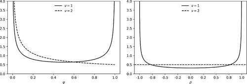
Figure 1 plots examples of priors for ψ and ρ for two obvious choices of ν. For ν = 1, the prior for ρ resembles (but is not identical to) the prior suggested in Lindley (1965), and the implied prior for γ is a Cauchy distribution (Crooks 2019). For ν = 2, the prior for ρ is uniform, as in (5). As ν becomes larger, the prior for ρ becomes narrower and the prior for γ becomes approximately normal.

Figure 1 Example priors for ψ (left panel) and ρ (right panel) for two choices of ν in (7).

Of course, it would be reasonable to object to privileging the correlation coefficient in this derivation of a prior distribution for γ. Instead, one could place a prior directly on γ, as in Leamer (1974). In fact, the approach outlined above was initially motivated as a way of justifying Leamer’s choice. In addition, it is worth noting that the generalized beta prior for ρ has the same form as many of the reference priors in Berger and Sun (2008), with the correspondence depending on the choice of ν.

5 Posterior Distributions for β

The model in Section 2 is only specified at the level of conditional expectation functions. To provide a more concrete guide to its applicability, consider the following hierarchical representation of a model that can be estimated in practice: (9) $$\begin{array}{cc}p(Y|\delta ,{\sigma }_V^2,x)\hfill & =\mathrm{N}\left(\delta x,{\sigma }_V^2\right),\hfill \\ \delta =\beta +\gamma ;p({\gamma }^{\mathrm{\star }}|{\sigma }_V^2,x)\hfill & =\text{St}\left(0,\frac{{\sigma }_V}{{\widehat{\sigma }}_X\sqrt{\nu }},\nu \right),\hfill \\ p({\delta }^{\mathrm{\star }},{\sigma }_V^{2\mathrm{\star }}|x)\hfill & \propto 1/{\sigma }_V^2.\hfill \end{array}$$(9)

The data are now assumed to be normally distributed, and both the data and priors are conditional on the sample values of the regressor. The prior distribution for the estimated regression parameters is uniform on $(\delta ,\hspace{0.17em}\log \hspace{0.17em}{\sigma }_V)$, that is, uninformative (Gelman et al. 1995, chap. 14).

Given the foregoing, the conditional posterior distribution for δ is normal, (10) $${\delta }^{\mathrm{\star }}|{\sigma }_V^2,y,x\sim \mathrm{N}\left(\widehat{\delta },\frac{{\sigma }_V^2}{s_{xx}}\right),$$(10) in which $\widehat{\delta }$ is the OLS estimator and s_xx is the sample sum of squares of the regressor, while the posterior for ${\sigma }_V^2$ is a scaled inverse-${\chi }^2$ distribution, (11) $${\sigma }_V^{2\mathrm{\star }}|y,x\sim \text{Inv}-{\chi }^2\left(n-1,{\widehat{\sigma }}_V^2\right),$$(11) in which ${\widehat{\sigma }}_V^2$ is the sample standard deviation of the OLS residuals.

As $\delta =\beta +\gamma$, the conditional posterior distribution for β is a convolution of the normal conditional posterior for δ and the Student’s t prior for γ, (12) $$\begin{array}{cc}{\beta }^{\mathrm{\star }}|{\sigma }_V,y,x\hfill & ={\delta }^{\mathrm{\star }}|{\sigma }_V,y,x\hfill \\ \hfill & -{\gamma }^{\mathrm{\star }}|{\sigma }_V,x.\hfill \end{array}$$(12)

As described in Pogány and Nadarajah (2013), the probability density function of this convolution can be expressed as, $$p(\beta )\propto \hspace{0.17em}\exp \hspace{0.17em}\left(-\frac{{\left(\beta -\widehat{\delta }\right)}^2}{\frac{2{\sigma }_V^2}{s_{xx}}}\right)\times g(\beta ),$$ in which $g(\beta )$ involves an integral that is explained in online appendix B, and is straightforward to evaluate numerically.

To compute the marginal posterior distribution for β, ${\sigma }_V^2$ needs to be integrated out of the conditional posteriors for δ and β in (12), using (11). This is straightforward to achieve using simulations, although certain choices of ν in the prior for γ might imply the need for a large number of runs to accurately estimate the tails in ${\gamma }^{\mathrm{\star }}|x$.

On the other hand, if both ν and the sample size are large enough, the marginal posteriors for both δ and γ will be approximately normal, and so too will the marginal posterior for β. These issues are considered further in the next section.

6 Practical Considerations

The model outlined in Section 5 is simplified to permit tractability, in order to aid pedagogy. However, if one can motivate a reasonable value for ν, then the model can be estimated. Moreover, the prior for $(\delta ,{\sigma }_V)$ could be changed without major complication (e.g., by using a conjugate prior).

How, then, should a researcher motivate a choice for ν? This will depend on the relationship being modeled and the presence of expert subject knowledge. But progress can be made by examining existing extreme bounds analyses in the relevant subject, to give some idea about the correlation structure of commonly used covariates (Leamer 1983).

Consider, for example, the problem of identifying the determinants of voter turnout in elections. This is of obvious policy importance, as the overall health of a democracy is closely related to the engagement of its citizens in the electoral process. Despite this, there is very little consensus in the political science literature on these determinants, mainly due to a lack of convincing identification strategies. One obvious possibility is the cross-country relationship between voter turnout and income inequality, (13) $$Y=\beta X+U,$$(13) in which Y denotes the number of voters in an election as a percentage of the voting population, and X denotes the Gini coefficient of income inequality. Clearly, $\mathrm{E}[U|X]=\gamma X$ in the general case.

This problem motivates the recent extreme bounds analysis in Frank and Martínez i Coma (2023). They estimate repeated linear regression models of the form described in (13), augmented with, (14) $$U=\zeta C+E,$$(14) in which C is a vector of different combinations of over 60 observable covariates, and E is an error term.

Using their dataset, the left panel of Figure 2 plots the empirical distributions of the squared correlation ψ between X and different choices of U, calculated from approximately 37,000 regressions (further details of the computations are provided in online appendix C). This histogram is overlaid with the beta prior in (7), in which $\nu =134$.

Figure 2 Empirical distribution of ψ from Frank and Martínez i Coma (2023) (left panel) and normal approximations to the posterior distributions for δ and β (right panel) in (13).

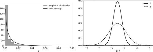
In this example, the empirical distribution of ψ is relatively tight. Moreover, the residual degrees of freedom in the simple linear regression of Y on X is 397, so one can treat the marginal posterior distributions of both δ and β as approximately normal. The posterior mean and variance for δ, using the model in Section 5, are–1.08 and 0.46, while the posterior for β is approximated by, (15) $${\beta }^{\mathrm{\star }}|y,x\sim \mathrm{N}\left(\widehat{\delta },\frac{{\widehat{\sigma }}_V^2}{s_{xx}}+\frac{{\widehat{\sigma }}_V^2}{{\widehat{\sigma }}_X^2\nu }\right),$$(15) which has a mean and variance of–1.08 and 1.83. Approximately 79% of this posterior mass is for negative values of β, with the remaining 21% positive.

These normal approximations to the posterior distributions of δ and β are displayed in the right panel of Figure 2. The increased uncertainty surrounding the treatment effect β compared to the reduced form δ is readily apparent, which is qualitatively similar to the results in Frank and Martínez i Coma (2023), in which the extreme bounds distribution of the coefficient on income inequality varies widely across model specifications.

The normal approximation in (15) illustrates in a particularly clear manner that the posterior standard deviation of β shrinks to a positive constant as the sample size increases, rather than zero. In general, as discussed Gustafson (2005), Moon and Schorfheide (2012), Gustafson (2015), and others, the posterior of the identified δ tends to the true value of δ as the sample size increases, while the posterior of the unidentified β tends to its conditional prior evaluated at the true value of δ.

Of course, in other cases a choice of large ν might be inappropriate. Moreover, one might be concerned that, even though scores of observable confounders have been used to estimate the distribution of ψ in this example, the remaining unobservable confounders might follow a different distribution. In these cases researchers could utilize a uniform prior for ρ, appealing to the principle of insufficient reason, or even the extreme prior obtained by setting ν = 1, which implies that the posterior for β is the convolution of a normal distribution and a Cauchy distribution, which is a Voigt distribution (Crooks 2019).

7 Discussion

According to the data visualization pioneer Edward Tufte, one of the “shortest true statements” that can be made about statistics is that, “correlation is not causation but it sure is a hint” (Tufte 2006). This outlook informs various approaches to statistics that attempt to deal with imperfect identification, including the literatures on unidentified regression models, imperfect instrumental variables, and sensitivity analysis.

In this article, I hope to have contributed to these literatures by providing a tractable approach to Bayesian inference for unidentified linear regression models. Although the estimation problem discussed in this paper does not disappear as the sample size increases, it does disappear as the correlation between the regressor and regressand becomes stronger, and σ_V approaches zero in (4). Simply put, the stronger the correlation between the regressor and regressand, the greater the likelihood of a positive treatment effect.

The results in this paper are most closely related to those in Leamer (1974) and Cinelli and Hazlett (2020). In fact, thinking about how one might appeal to the principle of insufficient reason to motivate a choice of variance for the bias prior in Leamer (1974) was the original inspiration behind this article, and was made possible by the derivations in Cinelli and Hazlett (2020). Various contributions in the medical statistics literature, including Gustafson (2005, 2009, 2010, 2012, 2014), McCandless, Gustafson, and Levy (2007, 2008), Gustafson et al. (2010), Xia and Gustafson (2016), and Gustafson and McCandless (2018), are also closely related.

Importantly, the Bayesian approach should not be seen as a competitor to sensitivity analyses, but rather a complement. In fact, one could conduct a sensitivity analysis on the Bayesian approach outlined in this article, by observing how the posterior for β changes when ν is varied deterministically. At the same time, using prior distributions can simply the inferential procedure somewhat, by reducing the amount of parameters that have to be varied deterministically.¹

Finally, there are many ways that the approach outlined in this article could be extended to make it less focused on simplicity for pedagogical reasons, and more focused on practical application. One obvious avenue is an extension to multiple linear regressions with observable controls, perhaps borrowing from the frequentist approach in Oster (2019). Another would be an exploration of the correlation structure of observable covariates using other extreme bounds analyses, or novel databases.

In any case, I hope that the tractability of the results presented here will help those unfamiliar with the literature to understand the peculiar problems of estimation and inference in unidentified models, and apply simple solutions in practice.

Supplementary Materials

Supplementary materials include a derivation of the bias parameter, an explanation of the convolution of a normal distribution and t-distribution, and further details on the empirical example.

Acknowledgments

I would like to thank Carlos Cinelli, Gavin Crooks, Andrew Gelman, Sander Greenland, Paul Gustafson, Karsten Kohler, Edward Leamer, Lawrence McCandless, Ron Smith, Rafael Wildauer, the editor and referees for very helpful feedback and suggestions. Any remaining errors are the responsibility of the author.

Disclosure Statement

This article did not receive specific funding, and the author has no competing interests to declare.

Notes

1 The argument that sensitivity analysis should be agnostic to inferential procedure was originally put to me by Carlos Cinelli, in private correspondence.

References

- Ashley, R. A., and Parmeter, C. F. (2015), “When Is It Justifiable to Ignore Explanatory Variable Endogeneity in a Regression Model?” Economics Letters, 137, 70–74. DOI: 10.1016/j.econlet.2015.09.029.
- Berger, J. O., and Sun, D. (2008), “Objective Priors for the Bivariate Normal Model,” The Annals of Statistics, 36, 963–982. DOI: 10.1214/07-AOS501.
- Burstyn, I., Barone-Adesi, F., De Vocht, F., and Gustafson, P. (2019), “What to Do When Accumulated Exposure Affects Health but Only Its Duration Was Measured? A Case of Linear Regression,” International Journal of Environmental Research and Public Health, 16, 1896. DOI: 10.3390/ijerph16111896.
- Chan, J. C., and Tobias, J. L. (2015), “Priors and Posterior Computation in Linear Endogenous Variable Models with Imperfect Instruments,” Journal of Applied Econometrics, 30, 650–674. DOI: 10.1002/jae.2390.
- Cinelli, C., and Hazlett, C. (2020), “Making Sense of Sensitivity: Extending Omitted Variable Bias,” Journal of the Royal Statistical Society, Series B, 82, 39–67. DOI: 10.1111/rssb.12348.
- Cornfield, J., Haenszel, W., Hammond, E. C., Lilienfeld, A. M., Shimkin, M. B., and Wynder, E. L. (1959), “Smoking and Lung Cancer: Recent Evidence and a Fiscussion of Some Questions,” Journal of the National Cancer Institute, 22, 173–203.
- Crooks, G. E. (2019), “Field Guide to Continuous Probability Distributions,” Technical Report, Berkeley Institute for Theoretical Sciences. Available at http://threeplusone.com/fieldguide
- DiTraglia, F. J., and Garcia-Jimeno, C. (2021), “A Framework for Eliciting, Incorporating, and Disciplining Identification Beliefs in Linear Models,” Journal of Business & Economic Statistics, 39, 1038–1053. DOI: 10.1080/07350015.2020.1753528.
- Dubs, H. H. (1942), “The Principle of Insufficient Reason,” Philosophy of Science, 9, 123–131. DOI: 10.1086/286754.
- Florens, J., Mouchart, M., and Rolin, J. (1985), “On Two Definitions of Identification,” Statistics: A Journal of Theoretical and Applied Statistics, 16, 213–218.
- Florens, J., Mouchart, M., and Rolin, J. (1990), Elements of Bayesian Statistics, Monographs and Textbooks in Pure and Applied Mathematics, Boca Raton, FL: CRC Press.
- Frank, K. A. (2000), “Impact of a Confounding Variable on a Regression Coefficient,” Sociological Methods & Research, 29, 147–194. DOI: 10.1177/0049124100029002001.
- Frank, R. W., and Martínez i Coma, F. (2023), “Correlates of Voter Turnout,” Political Behavior, 45, 607–633. DOI: 10.1007/s11109-021-09720-y.
- Gelman, A. (2006), “Prior Distributions for Variance Parameters in Hierarchical Models,” comment on article by Browne and Draper, Bayesian Analysis, 1, 515–534. DOI: 10.1214/06-BA117A.
- Gelman, A., Carlin, J. B., Stern, H. S., and Rubin, D. B. (1995), Bayesian Data Analysis, Boca Raton, FL: Chapman and Hall/CRC. Available at http://www.stat.columbia.edu/∼gelman/book/
- Greenland, S. (2005), “Multiple-Bias Modelling for Analysis of Observational Data,” Journal of the Royal Statistical Society, Series A, 168, 267–306. DOI: 10.1111/j.1467-985X.2004.00349.x.
- ——(2021), “Invited Commentary: Dealing with the Inevitable Deficiencies of Bias Analysis - and All Analyses,” American Journal of Epidemiology, 190, 1617–1621.
- Gustafson, P. (2005), “On Model Expansion, Model Contraction, Identifiability and Prior Information: Two Illustrative Scenarios Involving Mismeasured Variables,” Statistical Science, 20, 111–140. DOI: 10.1214/088342305000000098.
- ——(2009), “What are the Limits of Posterior Distributions Arising from Nonidentified Models, and Why Should We Care?” Journal of the American Statistical Association, 104, 1682–1695.
- ——(2010), “Bayesian Inference for Partially Identified Models,” The International Journal of Biostatistics, 6, Article 17.
- ——(2012), “On the Behaviour of Bayesian Credible Intervals in Partially Identified Models,” Electronic Journal of Statistics, 6, 2107–2124.
- ——(2014), “Bayesian Inference in Partially Identified Models: Is the Shape of the Posterior Distribution Useful?,” Electronic Journal of Statistics, 8, 476–496.
- ——(2015), Bayesian Inference for Partially Identified Models: Exploring the Limits of Limited Data (Vol. 140), Boca Raton, FL: CRC Press.
- Gustafson, P., McCandless, L., Levy, A., and Richardson, S. (2010), “Simplified Bayesian Sensitivity Analysis for Mismeasured and Unobserved Confounders,” Biometrics, 66, 1129–1137. DOI: 10.1111/j.1541-0420.2009.01377.x.
- Gustafson, P., and McCandless, L. C. (2018), “When is a Sensitivity Parameter Exactly That?” Statistical Science, 33, 86–95. DOI: 10.1214/17-STS632.
- Hosman, C. A., Hansen, B. B., Holland, P. W., et al. (2010), “The Sensitivity of Linear Regression Coefficients’ Confidence Limits to the Omission of a Confounder,” The Annals of Applied Statistics, 4, 849–870. DOI: 10.1214/09-AOAS315.
- Imbens, G. W. (2003), “Sensitivity to Exogeneity Assumptions in Program Evaluation,” American Economic Review, 93, 126–132. DOI: 10.1257/000282803321946921.
- Jeffreys, H. (1961), Theory of Probability (3rd ed.), New York: The Clarendon Press, Oxford University Press.
- Kadane, J. (1974), “The Role of Identification in Bayesian Theory,” in Bayesian Econometrics and Statistics, eds. S. Fienberg, and A. Zellner, Amsterdam: North Holland.
- Kiviet, J. F. (2016), “When Is It Really Justifiable to Ignore Explanatory Variable Endogeneity in a Regression Model?” Economics Letters, 145, 192–195. DOI: 10.1016/j.econlet.2016.06.021.
- Kraay, A. (2012), “Instrumental Variables Regressions with Uncertain Exclusion Restrictions: A Bayesian Approach,” Journal of Applied Econometrics, 27, 108–128. DOI: 10.1002/jae.1148.
- Leamer, E. (1974), “False Models and Post-Data Model Construction,” Journal of the American Statistical Association, 69, 122–131. DOI: 10.1080/01621459.1974.10480138.
- Leamer, E. E. (1983), “Let’s Take the Con Out of Econometrics,” The American Economic Review, 73, 31–43.
- Lindley, D. (1965), Introduction to Probability and Statistics from a Bayesian Viewpoint (Part 2: Inference), Cambridge, UK: Cambridge University Press.
- Ly, A., Marsman, M., and Wagenmakers, E.-J. (2018), “Analytic Posteriors for Pearson’s Correlation Coefficient,” Statistica Neerlandica, 72, 4–13. DOI: 10.1111/stan.12111.
- McCandless, L. C., Gustafson, P., and Levy, A. (2007), “Bayesian Sensitivity Analysis for Unmeasured Confounding in Observational Studies,” Statistics in Medicine, 26, 2331–2347. DOI: 10.1002/sim.2711.
- McCandless, L. C., Gustafson, P., and Levy, A. (2008), “A Sensitivity Analysis Using Information about Measured Confounders Yelded Improved Uncertainty Assessments for Unmeasured Confounding,” Journal of Clinical Epidemiology, 61, 247–255. DOI: 10.1016/j.jclinepi.2007.05.006.
- Moon, H. R., and Schorfheide, F. (2012), “Bayesian and Frequentist Inference in Partially Identified Models,” Econometrica, 80, 755–782.
- Novack, G. (2010), “A Defense of the Principle of Indifference,” Journal of Philosophical Logic, 39, 655–678. DOI: 10.1007/s10992-010-9147-1.
- Oster, E. (2019), “Unobservable Selection and Coefficient Stability: Theory and Evidence,” Journal of Business & Economic Statistics, 37, 187–204. DOI: 10.1080/07350015.2016.1227711.
- Pogány, T. K., and Nadarajah, S. (2013), “On the Convolution of Normal and t Random Variables,” Statistics, 47, 1363–1369. DOI: 10.1080/02331888.2012.694447.
- Poirier, D. (1998), “Revising Beliefs in Nonidentified Models,” Econometric Theory, 14, 483–509. DOI: 10.1017/S0266466698144043.
- Rosenbaum, P. R., and Rubin, D. B. (1983), “Assessing Sensitivity to an Unobserved Binary Covariate in an Observational Study with Binary Outcome,” Journal of the Royal Statistical Society, Series B, 45, 212–218. DOI: 10.1111/j.2517-6161.1983.tb01242.x.
- Tufte, E. (2006), The Cognitive Style of PowerPoint: Pitching Out Corrupts Within, Cheshire, CT: Graphics Press LLC.
- Wechsler, S., Izbicki, R., and Esteves, L. G. (2013), “A Bayesian Look at Nonidentifiability: A Simple Example,” The American Statistician, 67, 90–93. DOI: 10.1080/00031305.2013.778787.
- Wooldridge, J. M. (2010), Econometric Analysis of Cross Section and Panel Data, Cambridge, MA: MIT Press.
- Xia, M., and Gustafson, P. (2016), “Bayesian Regression Models Adjusting for Unidirectional Covariate Misclassification,” Canadian Journal of Statistics, 44, 198–218. DOI: 10.1002/cjs.11284.