Renewable energy resource integrated multilevel inverter using evolutionary algorithms

Abstract

In this paper, with the development of an intelligent power system idea, sustainable energy sources were increasingly deployed, including transmission and distribution systems networks. As a result, optimal use of cascaded H-bridge inverter topologies (MLIs) and power distribution operations is critical for long-term power generation. Traditionally, selective harmonics reduction models must be performed to achieve the optimal switching frequency of multilevel inverters. This research aims to determine the switching frequency for wind-incorporated multilevel inverters to reduce overall harmonic components used in grid applications. This research adds towards the best possible solution by employing multiple newly established adaptive optimization techniques: MNSGA-II and salp swarm. The well-known genetic algorithm and particle swarm optimization are used for the wind-tied multilevel inverters optimization issue. Seven-level, eleven-level, and fifteen-level MLIs were employed to reduce overall harmonic distortion. The reliability and convergence rate of simulated data with various modulation indices for seven-, eleven-, and fifteen-level MLIs are obtained and compared. Models are developed based on MATLAB Simulink and are used to validate quantitative measurements.

KEYWORDS:

• Modified non-dominated sorting genetic algorithm (MNSGA-II)
• salp swarm algorithm (SSA)
• particle swarm optimization (PSO)
• multilevel inverters (MLIs)
• modulation index
• cascaded H-bridge

1. Introduction

The impacts of climate change on our planet are increasingly becoming a serious threat. As stated in the Paris climatic accord of 2015, the world is committed to keeping the global temperature increase below 2 degrees Celsius. The primary contributor of this climate change is the burning of fossil fuels, which in turn releases large amounts of carbon dioxide into the atmosphere. To reduce the effects of climate change, the energy balance is being reformulated to include renewable and sustainable sources of energy, such as biofuels [1].

To facilitate the integration of renewable sources of energy into the grid, several control techniques have been proposed. For example, a three-level inverter can be used to create a hierarchical optimum multi-objective control scheme, wherein the grid side and neutral-point voltages are optimized using fuzzy satisfaction determination [2]. On the other hand, genetic algorithms have been used to generate an optimal solution to the state-of-charge equations [3]. However, the classic FCS-MPC technique suffers from a large number of sliding optimization computations and difficulties in coefficient calculation. To address this, an optimal model predictive control technique has been developed that reduces the number of switching stages and simplifies the calculation of weight factors. Additionally, active damping has been proposed to mitigate the resonance of LC filters without the need for additional physical equipment, thereby increasing the controller versatility [4,5].

The modelling and implementation of an all-silicon hyper-efficient discreetly ventilated 12.5-kilowatt three-phase seven-stage Hybrid Active Neutral Point Clamped inverters and the testing of the project of maximum efficiency and energy densities. By utilizing a DC-bus midpoint connection and an active neutral point clamped level front-end that employs switching designed at twice the Voltage level and operates online frequency, the number of flying capacitor units can be significantly reduced, especially in lower frequency variation, resulting in better-efficient converters [6]. The Probabilistic approach is then used to compute the maintenance costs based on the frequency of experiencing the stages, incorporating the upfront outlay, components power dissipation, maintenance power loss, replacement costs, and external conditions into a single indicator [7]. A centralized BESS siting optimum algorithm based on a no-preference proposed method employing an evolutionary algorithm that examines a global optimum determined using engineering and commercial characteristics is also employed [8]. Furthermore, approaches for reduced switching carrier frequency, including harmonic distortion reduction, provide essential benefits such as minimal transmission loss, flexibility control terminal voltage oscillations, and an excellent harmonic frequency pattern [9,10]. A non-dominated sorting Multi-Objective Grey Wolf Optimizer is then utilized to fix the multi-objective structure of an optimal solution and is compared using NSGA-II [11]. The fundamental input analyses, modelling, and experimental findings have thus confirmed the feasibility of the developed Elongated Multilevel Inverters, and the power supply issue is well accepted by employing the Multi-Objective Grey Wolf Optimizer-based restructuration harmonics removal technique.

Harmonic distortion definitions and its application to multilevel inverters of various architectures would be incomplete without a discussion of the hybrid active filter using the bidirectional converter control approach and the cascaded H-bridge configuration [12]. This approach has the advantage of providing reactive power and speed control for doubly fed induction machines [13]. In addition, the probabilistic structure of wind turbine and photovoltaic production and varying loads has been used to develop the best possible power converter Solar, WT, and Battery storage systems [14]. Furthermore, the use of Social Spider Optimizer has been suggested as it requires fewer regulating variables and is easy to implement [15]. The author's proposed architecture for removing the requirement for additional controls in capacitor voltage equalization and the necessity for power frequencies of transformers is based on the Cascaded multilevel inverters design that enables the use of the entire dc-link voltage [16]. This control technique has been evaluated in terms of converters current as well as high-voltage direct link voltage limits, as well as positively and negatively sequences grids codes need under extreme stable and unstable disturbances just at the point of common coupling of alternating grids [17]. The feedforward voltages and current circuits can be used to regulate the bus voltage of photovoltaic systems and introduce voltage faults into a solitary reference signal [18]. The efficiency of Asynchronous Particle Swarm Optimization-GA in terms of higher accuracy and the chance of reaching global optimal solutions has been tested using the cumulative distribution function to evaluate the fitness values obtained using different algorithms [19]. Additionally, the modified grey wolf optimization has been integrated with other inverter topologies to test its performance based on harmonic indices and convergence rate.

Recent studies have proposed a single-stage MLI architecture to reduce the number of transistors inside the circuits and attain higher reference voltages at outputs [20]. The architecture also provides more levels at outputs using many switching DC sources [21]. An industrial IoT algorithm was used to monitor the wind energy system using IoT [22], while a freestanding Solar panel was used that employed a 21-stage multilevel inverter combined with a three-stage DC-DC power converter [23]. Dissent quantization bat metaheuristic method was used to tackle the non-linear Pulse width modulation problem [24,25]. This strategy utilizes the features of permanent magnet synchronous generators (PMSG) and cascaded H-bridge STATCOMs (CHBs) to separate the active and reactive power control of the grid-connected converters, thus reducing the unbalanced voltage. The proposed strategy was validated through simulations and experiments on a laboratory setup and was found to effectively reduce unbalanced grid voltage and improve the power quality of the grid [26].

According to the literature study, the MNSGA-II and salp swarm optimization function well when addressing technological difficulties. As a result, this work builds on the earlier investigation of either the model employed or the methods utilized. It employs salp swarm optimization and MNSGA-II to eliminate distortions and minimize harmonic distortion in the multilevel inverter. Various realistic numerical simulations of wind-tied multilevel inverters for seven, eleven, and fifteen levels were determined and compared employing MNSGA-II and salp swarm optimization. Simulation models also utilize GA and Swarm optimization, a well-known community optimal approach. Proposed algorithm, MNSGA-II and salp swarm algorithms, are extensions of GA and PSO. Despite this, our approach is novel in several respects. First, we introduce the concept of a “multi-objective non-dominated sorting genetic algorithm-II” (MNSGA-II). This algorithm combines the best of both GA and PSO, while still maintaining the multi-objective nature of the problem. Second, we propose the use of a “Salp Swarm Algorithm” to further optimize the performance of the algorithm. This approach has not been previously used in the field and could potentially lead to substantial improvements in the performance of the algorithm. Finally, here we conducted extensive experiments using real-world datasets to demonstrate the efficacy of our approach. This provides further evidence of the novelty of our approach. The mathematical computations’ findings are validated utilizing Matlab / Simulink software modelling. In summary, the following are the original study achievements:

• An optimal control model eliminates distortions and minimizes total harmonic distortions.

• The optimal control solution is obtained using the salp swarm algorithm and MNSGA-II. The results obtained of 7-level, 11-level, and 15-level Wind tied. Multilevel inverter models were evaluated through analytical reliability and precision. Furthermore, the mathematical findings from MNSGA-II and SSA are contrasted towards the results derived via GA and PSO.

• MATLAB Simulink modelling for a seven-level wind-connected multilevel inverter is created. Harmonic distortion calculations are performed with the Fourier tool and compared to those produced with heuristics optimization algorithms.

The following is an outline of the article's body: The Overview of the multilevel inverters with suggested cascaded H-bridge is described in Chapter 2. Chapter 3 defines the Wind System Model with an Uncontrolled diode bridge rectifier in detail. Chapter 4 defines the Heuristic methods with different optimization like MNSGA-II, Salp swarm, GA, and PSO to assess the system's total response for each MLIs component and its initial transfer function and appropriate cost measurements. Chapter 5 comprehensively describes the proposed system's real-time development and performance evaluation. And thus, the suggested method's outcomes and comments are analysed. Eventually, Chapter 6 concludes the article.

2. Multilevel inverters with suggested cascaded H-bridges

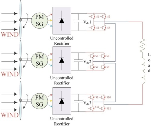
Figure 1 is a simplified representation of a cascaded H-bridge multilevel inverters having 7 layers. This should be noted that the amplitudes of the DC supplies were equivalent and linked towards a renewable wind source, single-phase full-bridge converter, and H-bridge inverters. Dependent on how the Input voltages are connected towards the AC outputs, every inverter stage generates +V_in, 0, or –V_in. This should be noticed that the configurations of switching devices S_w have a vital role throughout the outputs. Generally, the higher the number of levels and the more complex the modulation technique, the higher the switching frequency. The switching frequency also depends on the desired level of power quality, as higher switching frequencies tend to reduce ripple and noise in the output voltage. In general, switching frequencies for multilevel inverters can range from a few kilohertz to hundreds of kilohertz. The proposed work is done through 200 KHz.

Figure 1. Multilevel inverter with a single-phase and 7 levels of suggested cascaded H-bridge.

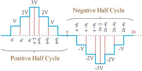
The range of output voltages depends on the number of independent DC supplies and can be expressed by 2*t + 1; wherein t seems to be the range of different DC supplies. The FFT of stepped waveforms of s stages is seen as follows. The stepping terminal voltage graphs of 7-level inverters and their related conduction angles are illustrated in Figure 2. The fundamental multilevel inverter relations are represented in Equations (1(1) $\begin{array}{rl}V\left(\mathrm{\omega T}\right)& =\frac{4V_{\mathrm{in}}}{\pi }\sum _m[\cos m{\varphi }_1+\cos m{\varphi }_2+\dots \\ & +\cos m{\varphi }_s]\sin \frac{\mathrm{m\omega T}}{m};m=1,3,5,\mathrm{7..}\end{array}$(1) ) to (5(5) $\begin{array}{rl}G\left(7m\right)& =\cos 7{\varphi }_1+\cos 7{\varphi }_2+\cos 7{\varphi }_3\end{array}$(5) ) [27]. (1) $\begin{array}{rl}V\left(\mathrm{\omega T}\right)& =\frac{4V_{\mathrm{in}}}{\pi }\sum _m[\cos m{\varphi }_1+\cos m{\varphi }_2+\dots \\ & +\cos m{\varphi }_s]\sin \frac{\mathrm{m\omega T}}{m};m=1,3,5,\mathrm{7..}\end{array}$(1) Equation (1), $\omega$ as well as $V_{\mathrm{in}}$ correspondingly, the DC input's rotation speed and output voltages. Take note as ${\varphi }_j$ represents the conduction angles of stage j. When applying $V_{\mathrm{in}}$ normalization, the difference of the components in Equation (1) Maybe calculated using the standard representation (2) $\begin{array}{rl}G\left(m\right)& =\frac{4}{\mathrm{m\pi }}\sum _m[\cos m{\varphi }_1+\cos m{\varphi }_2+\dots \\ & +\cos m{\varphi }_s];m=1,3,5,\mathrm{7..}\end{array}$(2) Wherein it's switching orientations ${\varphi }_1$, ${\varphi }_2$, … , ${\varphi }_m$ should fulfil the following constrictions: (3) $\begin{array}{r}{\varphi }_1\le {\varphi }_2\le \dots \le {\varphi }_m\le \frac{\pi }{2}\end{array}$(3)

Figure 2. Seven-level cascaded H-multilevel bridge's inverter voltage outputs.

Total harmonic distortion is determined as the percentage of the summing of voltage measurement having odd indices towards the required power components, which may be expressed quantitatively as, (4) $\begin{array}{r}\text{THD}=\frac{\sqrt{{\sum }_{m=3,5,7\dots }^{m=49}{V}_m^2}}{V_1^2}\end{array}$(4)

Traditionally, optimizing methods are designed to decrease reduced-order harmonic components. Such a technique is outlined simply below. The amount of distortions that may be removed is smaller than the total of H-bridges. $\begin{array}{rl}G\left(m\right)& =\cos {\varphi }_1+\cos {\varphi }_2+\cos {\varphi }_3-3n_1\end{array}$ $\begin{array}{rl}G\left(5m\right)& =\cos 5{\varphi }_1+\cos 5{\varphi }_2+\cos 5{\varphi }_3\end{array}$ (5) $\begin{array}{rl}G\left(7m\right)& =\cos 7{\varphi }_1+\cos 7{\varphi }_2+\cos 7{\varphi }_3\end{array}$(5) $n_1$ Seems to be the modulation indices defined through (5) as $\frac{V_l^{\ast }}{V_{\mathrm{lmax}}}$. This should be noted as $V_l^{\ast }$ indicates the inverter's magnitude commands for only a sinusoidal waveform outputs voltage level whereas $V_{\mathrm{lmax}}$ denotes the inverter's optimum value magnitude. To eliminate the uneven oscillations, $G\left(k\right)$ values ought to be equivalent to 0. Nevertheless, because the IEEE 519 typical requires its first 50 harmonics to be minimized, this study incorporates various approaches to optimize 7, eleven, and fifteen Multilevel inverters: (6) $\begin{array}{rl}& \text{minimise}\sqrt{\frac{{\sum }_{m=3,5,\mathrm{7..}}^{m=49}{V}_m^2}{V_1}}+|\cos {\mathrm{\Psi }}_1+\cos {\mathrm{\Psi }}_2+\dots \\ & +\cos {\mathrm{\Psi }}_k-\mathrm{Kn}|,\\ & \text{subject to }{\varphi }_1\le {\varphi }_2\le \dots \le {\varphi }_k\le \frac{\pi }{2}\end{array}$(6) Equation (6), k equals 3, 5, and 7 with seven-, eleven-, as well as fifteen-level multilevel inverters, correspondingly.

3. Wind system model with uncontrolled DBR

The wind generator produced electrical output at a specified nominal state based on wind direction. Therefore, the wind velocity is related to Equation (7(7) $\begin{array}{rl}{P}_{\mathrm{wind}}& =\{\begin{array}{l}0,V〈V_{\mathrm{Cin}}\left(\mathrm{or}\right)V〉V_{\mathrm{Cout}}\\ P_{\mathrm{wind}}^{\max }\left(\frac{P_{\mathrm{wind}}^c-P_{\mathrm{wind}}^{\max }}{V_{\mathrm{Cout}}-V_R}\right)\left(V\left(t\right)-V_R\right)\\ P_{\mathrm{wind}}^{\max }\left(\frac{V\left(t\right)-V_{\mathrm{Cin}}}{V_R-V_{\mathrm{Cin}}}\right)\text{3,}{V}_{\mathrm{Cin}}\le V\le V_R\end{array},\\ & V_R<V\le V_{\mathrm{Cout}}\end{array}$(7) ) depending on the wind generator [28]. (7) $\begin{array}{rl}{P}_{\mathrm{wind}}& =\{\begin{array}{l}0,V〈V_{\mathrm{Cin}}\left(\mathrm{or}\right)V〉V_{\mathrm{Cout}}\\ P_{\mathrm{wind}}^{\max }\left(\frac{P_{\mathrm{wind}}^c-P_{\mathrm{wind}}^{\max }}{V_{\mathrm{Cout}}-V_R}\right)\left(V\left(t\right)-V_R\right)\\ P_{\mathrm{wind}}^{\max }\left(\frac{V\left(t\right)-V_{\mathrm{Cin}}}{V_R-V_{\mathrm{Cin}}}\right)\text{3,}{V}_{\mathrm{Cin}}\le V\le V_R\end{array},\\ & V_R<V\le V_{\mathrm{Cout}}\end{array}$(7) $P_{\mathrm{wind}}^c$ denotes wind turbines at cutting voltages, V_R denotes baseline wind velocity, V(t) denotes wind velocity at time t, $V_{\mathrm{Cout}}$ denotes windmill cutoff speed, $V_{\mathrm{Cin}}$ denotes windmill cut-in speed, and $P_{\mathrm{wind}}^{\max }$ denotes wind creates maximum power. However, the turbine's mechanical output may be tuned towards any power depending on the known wind velocity via changing those variables on such a network, solar and wind technologies moderate peak load. When the generation capacity exceeds the ability of hybrid energy systems to regulate, a battery can be connected to the system. Due to its robust control techniques, the wind speed remains constant at various ecological conditions. The literature illustrates that the bridge rectifier rectifies the input using diodes. Because the diode is a unidirectional circuit, the current can only travel in one way. This diode design inside the rectifier doesn't enable the power to fluctuate based on the load demand. As a result, this rectifier is found in continuous or fixed power sources.

4. Heuristic methods

The chapter defines the heuristics strategies used only to solve the Harmonic distortion elimination issue. The first paragraph discusses the MNSGA-II method and steps to implement a Harmonic distortion reduction issue. Furthermore, the SSA, GA, and PSO approaches were recently explained in the subsequent paragraphs. Finally, the procedures and schematics are provided to demonstrate how the approaches are applied towards the Harmonic distortion elimination issue.

4.1. Modified non-dominated sorting genetic algorithm MNSGA-II

The NSGA-II techniques benefited elitism, non-dominance, selection, and crowding closeness, which resulted in rapid convergence to the best method. Several publications have previously addressed the NSGA-II. The improved NSGA-II, which incorporates Pareto optimum searching, deals with inequality, quick non-dominated sorting, and variation. As a result, transverse diversity is stable, and non-dominated reinforcement is consistently delivered to the Pareto front. To solve this limitation, a new non-dominated sorting evolutionary algorithm (MNSGA-II) was developed to increase non-dominated variants arrangements due to the nonlinear crowding distance. The following Equation (8(8) $\begin{array}{r}c{d}_i=\frac{1}{r}\sum _{k=1}^r|h_{i+1}^k-h_{i-1}^k|\end{array}$(8) ) is the crowding distance equation: (8) $\begin{array}{r}c{d}_i=\frac{1}{r}\sum _{k=1}^r|h_{i+1}^k-h_{i-1}^k|\end{array}$(8) where cd_i is the crowding distance of an ith solution, denotes the number of objectives, as well as $h_i^k$ is still the kth target value of the ith solution. The issue with this approach is that there is an insufficient homogenous variation to discover the optimal answer. The MNSGA-II procedures would utilize $\mathrm{dcd}$ methods to overcome glitches of the proposed problem and it is represented in Equation (9(9) $\begin{array}{r}\mathrm{dc}{d}_i=\frac{c{d}_i}{\log \left(1/\phantom{1V_i}{V}_i\right)}\end{array}$(9) ). (9) $\begin{array}{r}\mathrm{dc}{d}_i=\frac{c{d}_i}{\log \left(1/\phantom{1V_i}{V}_i\right)}\end{array}$(9)

The particular variation of the $\mathrm{cds}$ with the neighbour of the ith solution provides information about the various degrees of $\mathrm{cd}$ in different applications represented in Equation (10(10) $\begin{array}{r}{V}_i=\frac{1}{r}\sum _{k=1}^r(|h_{i+1}^k-h_{i-1}^k|-c{d}_i{)}^2\end{array}$(10) ). (10) $\begin{array}{r}{V}_i=\frac{1}{r}\sum _{k=1}^r(|h_{i+1}^k-h_{i-1}^k|-c{d}_i{)}^2\end{array}$(10) Whenever the $\mathrm{dcd}$ method is utilized, the non-dominated sorting strategy is adjusted. The planned MNSGA-II, which includes $\mathrm{dc}{d}^{\mathrm{\prime }}s$ stages-specific process flow, is shown below.

• Stage 1: Estimate the Control Variable that is likely to be the output voltage.

• Stage 2: Specify parameters such as the population size, the maximum number of iterations, and the likelihood of mutation and crossover.

• Stage 3: Generate a starting population and assess the goal parameters.

• Stage 4: Establish the generation count i = 0.

• Stage 5: Perform binary crossover as well as polynomial mutation tests.

• Stage 6: Order the merged parent and offspring populations utilizing non-dominated sorting.

• Stage 7: Develop a population in subsequent generations using DCD from a combined parent and offspring population.

• Stage 8: Select your parents based on your tournament ranking.

• Stage 9: i < i_max.

In conclusion, MNSGA-II diversity and the Pareto optimal front are created with high consistency.

4.2. Genetic algorithm

An optimization strategy is a comprehensive search that may address complicated problems and optimize tough jobs. GA uses randomized transition rules instead of deterministic assumptions to develop communities of plausible possibilities known as chromosomes over and over again. Almost every stage of an algorithm is referred to as an iteration. To simulate systems integration, goal functions and genetic algorithms such as reproduction, crossover, and mutation are utilized. As seen, an optimization method is frequently initiated with a population of people. Every population is strongly mentioned by a chromosome, a unique binary sequence. The objective function evaluates and examines a person's knowledge via allocating a similar value called its performance to each individual. The stability of each chromosome is assessed, and a selection of the fittest approach is utilized. In this work, the error signal is used to determine the fitness of each chromosome. The three primary activities of evolutionary computation are reproduction, crossover, and mutation [29].

• Stage 1: Set the parameters using a random set of values, such as the crossover probability, number of iterations, number of nodes, and reproductions ratios. Choose a coding method.

• Stage 2: Determine and evaluate the results of the fitness function.

• Stage 3: Proceed with the mutation and crossover procedures until the full cluster is implemented.

• Stage 4: Stage 2 should be performed again until desired results are obtained.

It uses a Genetic Algorithm to Optimize MLI parameters. It has been summarized further down. GA initially generates randomized populations, which are then applied with a small population adequate to allow the controllers to be tweaked and convergence to occur faster. The initial population is obtained by transforming the MLIs parameters into binary representation known as chromosomes. Next, the viability of each chromosome is calculated by converting its binary text into an actual number that provides the MLIs parameters. Finally, every pair of MLI parameters is sent to the MLI for fixing the switching angles. To assess the system's total response for each MLI component and its initial transfer function, appropriate cost measurements such as ISE, IAE, and ITAE, as well as a weighted combination of these three cost functions, are utilized. This technique would be repeated until the greatest fitness level is reached at the end of the generation. The primary purpose of GA is to determine the global parameters that have the lowest optimum solution for running the plants throughout the whole array. Table 1 summarizes the GA variables used in the simulations.

Table 1. GA specifications utilized in the simulation.

Parameters	Values/Ranges
Maximum generations	113
Encoding	Binary
Population size	19
Crossover	1-point
Mutation	Uniform
Selection	Uniform

Following mutations, the GA computes the optimal solution using the Fitness Functions (FF). Therefore, one of the most crucial issues is to evaluate the fitness values of every chromosome. Since the finest chromosomes are determined by taking this into account and are saved from correlating with the finest chromosomes in the following group. As a result, the FF should be specified correctly to select the finest chromosome with the lowest Total of Harmonic Distortion. (11) $\begin{array}{r}\mathrm{ff}=\frac{\sqrt{{\sum }_{\left(\mathrm{odd}\right)m=3,5}^f\left(\frac{1}{m^2}{\sum }_{k=1}^{\frac{f+1}{2}}{\left(\cos m{\mathrm{\Psi }}_k\right)}^2\right)}}{\left|{\sum }_{k=1}^{\left(f+1\right)/2}\left(\cos {\mathrm{\Psi }}_k\right)\right|}\end{array}$(11) Wherein “f” is the highest degree of harmonics to be eliminated. “f” could also be written as 2k – 1. Ultimately, after every repetition, GA evaluates the objective value of every chromosome and selects the most suitable chromosomes via analysing the following iterative approach. The finest chromosomes are picked in the final repetition, and switching angles were calculated in radians.

4.3. Particle swarm optimization

PSO is based mainly on the swarming behaviour of bird flocks in search of food [30]. The approach takes inputs from the shortest local and global choices. Consequently, particles were anticipated to migrate to locations near-optimal places. Each repeat utilizes the positional modification technique, which is based on the mathematical model: (12) $\begin{array}{rl}{P}_{\mathrm{sd}}& =\left(w\ast P_{\mathrm{sd}}\right)l_1\ast \mathrm{random}\mathrm{number}\\ & \ast (\mathrm{local}\mathrm{finest}-P_{\mathrm{dr}})+l_2\ast \mathrm{random}\mathrm{number}\\ & \ast (\mathrm{global}\mathrm{finest}-P_{\mathrm{dr}})\end{array}$(12)

In Equation (12(12) $\begin{array}{rl}{P}_{\mathrm{sd}}& =\left(w\ast P_{\mathrm{sd}}\right)l_1\ast \mathrm{random}\mathrm{number}\\ & \ast (\mathrm{local}\mathrm{finest}-P_{\mathrm{dr}})+l_2\ast \mathrm{random}\mathrm{number}\\ & \ast (\mathrm{global}\mathrm{finest}-P_{\mathrm{dr}})\end{array}$(12) ), $l_1$ and $l_2$ represent the training constants, whereas $P_{\mathrm{sd}}$ and $P_{\mathrm{dr}}$ represent the particle's speed and direction, respectively. As explained previously, the speed gets revised by utilizing the best local and global factors. Those are referred to as the “local finest” and the “global finest”. Once the speeds have been determined, the locations may be simply modified utilizing quadratic formulas: (13) $\begin{array}{r}{P}_{\mathrm{sd}}=P_{\mathrm{sd}}+P_{\mathrm{dr}}\end{array}$(13)

The phases of the particle swarm technique for finding the best solution for inverters are as follows:

• Stage 1: The beginning entails determining the control parameters and initializing the elements. The particles, as well as the training parameters $l_1$ and $l_2$, were taken into account. Based on the intensity of the inverters under investigation, each particle is composed of three, five, or seven values. Consequently, the components of all particles should satisfy the standard condition: 0 ≤ θ ≤ π/2.

• Stage 2: The best local and global targets are then established to calculate each particle's model parameters.

• Stage 3: The particle speeds were changed utilizing Equation (12(12) $\begin{array}{rl}{P}_{\mathrm{sd}}& =\left(w\ast P_{\mathrm{sd}}\right)l_1\ast \mathrm{random}\mathrm{number}\\ & \ast (\mathrm{local}\mathrm{finest}-P_{\mathrm{dr}})+l_2\ast \mathrm{random}\mathrm{number}\\ & \ast (\mathrm{global}\mathrm{finest}-P_{\mathrm{dr}})\end{array}$(12) ) by employing training parameters and the local and global optimal outcomes. Eventually, Equation (13(13) $\begin{array}{r}{P}_{\mathrm{sd}}=P_{\mathrm{sd}}+P_{\mathrm{dr}}\end{array}$(13) ) is employed to alter the placements.

• Stage 4: To analyse the proposed grid-tied inverter's updated elements, including associated switching configurations. The findings are reported in the outcomes of the next iteration. The narrower the particles, the more particles which are preserved.

• Stage 5: The optimal solution is enhanced on a local and global basis.

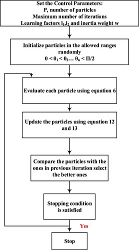
• Stage 6: This step decides whether or not the algorithm must be stopped. The stopping condition often investigates for reaching the number of iterations or analyses the quantitative differences between the finest ideally gained thus far and those obtained in a previous iteration. The algorithms create the phase angle if the option is to stop; otherwise, it returns to the third phase. Figure 3 displays the PSO flowchart for determining the optimal solution for inverters.

Figure 3. Diagrammatic flow of the PSO algorithm.

4.4. Salp swarm algorithm

SSA replicates the swarm behaviour of salps throughout the optimization procedure [31]. Salps develop salp networks to facilitate their movement while also making it easier to obtain food supplies. Viable alternatives, such as other heuristic techniques, are crucial to finding solutions. As a result, numerous others try to imitate the best salp, known as the chain's main salp. The next salp's purpose is to find the best response or the food supply. As a result, at the end of the operation, all members of the salp community were expected to move to the best option. Positioning changes of the significant salps and followers are performed utilizing Equations (14(14) $\begin{array}{r}{y}_i^1=\{\begin{array}{c}{G}_i+d_1\left(u{b}_i-l{b}_i\right)d_2+l{b}_i{d}_3\ge 0\\ G_i-d_1\left(u{b}_i-l{b}_i\right)d_2+l{b}_i{d}_3\ge 0\end{array}\end{array}$(14) ) to (16(16) $\begin{array}{r}{y}_i^1=\frac{1}{2}{V}_p{t}^2+V_{0}t\end{array}$(16) ), given below. (14) $\begin{array}{r}{y}_i^1=\{\begin{array}{c}{G}_i+d_1\left(u{b}_i-l{b}_i\right)d_2+l{b}_i{d}_3\ge 0\\ G_i-d_1\left(u{b}_i-l{b}_i\right)d_2+l{b}_i{d}_3\ge 0\end{array}\end{array}$(14) while $y_i^1$ is the leading salp, $G_i$ is the food supply positioning, $u{b}_i$ and $l{b}_i$ are top and bottom bounds, and d₁, d₂, and d₃ are randomized integers. The variable $d_1$ is defined as follows in Equation (15(15) $\begin{array}{r}{d}_1=2e^{-{\left(\frac{4l}{L}\right)}^2}\end{array}$(15) ): (15) $\begin{array}{r}{d}_1=2e^{-{\left(\frac{4l}{L}\right)}^2}\end{array}$(15) while $1$ and $l$ are the current number of iterations and the maximum number of iterations, respectively, Newton's law of motion is used to update the location of the follower's salps: (16) $\begin{array}{r}{y}_i^1=\frac{1}{2}{V}_p{t}^2+V_{0}t\end{array}$(16) $V_0$ represents the initial speed in this scenario, and $V_p$ is calculated by dividing the final speed by the actual speed. The SSA technique for achieving the optimum inverter solution consists of several stages:

• Stage 1: At this point, the salps are generated. Every salp entry matches to a changing angle. Variables are loaded with randomly integer values within the acceptable tolerance. In other words, the number of salps was Ns, and each salp is comprised of s components ranging from 0 to π/2 that satisfy the condition: 0 ≤ θ ≤ π/2. The number of parameters in each salp would fluctuate for inverters.

• Stage 2: The inputs from each salp were fed into the inverter, and the best solution for every salp was determined.

• Stage 3: The proper solution among the solution aspirants is known as the leader. It is also identified by grouping the salps depending on the results of the best solution assessments. The other options, or followers, are expected to follow the leader. Equations (14(14) $\begin{array}{r}{y}_i^1=\{\begin{array}{c}{G}_i+d_1\left(u{b}_i-l{b}_i\right)d_2+l{b}_i{d}_3\ge 0\\ G_i-d_1\left(u{b}_i-l{b}_i\right)d_2+l{b}_i{d}_3\ge 0\end{array}\end{array}$(14) ) and (15(15) $\begin{array}{r}{d}_1=2e^{-{\left(\frac{4l}{L}\right)}^2}\end{array}$(15) ) are utilized to change the position of the leader.

• Stage 4: The equation is used to change the positions of the followers (16).

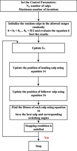
• Stage 5: This stage determines whether the strategy should be abandoned or continued. It analyses the variations between the best methods after a set number of iterations or compares the optimal solution. If the algorithms do not allow standstill, they go to stage 2. Figure 4 displays the flowchart of the SSA to inverter optimal solution execution.

Figure 4. The diagrammatic flow of the SSA algorithm.

4.5. Harmonic modelling

This section will discuss the various aspects of harmonic modelling for renewable energy resource-integrated multilevel inverter. Firstly, the harmonic content of the multilevel inverter output voltage must be determined. This can be done by using Fourier analysis, which is a method of decomposing a signal into its harmonic components. The harmonic content of the multilevel inverter output voltage can then be used to calculate the total harmonic distortion (THD) of the system. This is important as the THD of the system should be kept within certain limits, as defined by the relevant standards and regulations. Secondly, the transfer function of the multilevel inverter should be modelled. This can be done by using the state-space equations, which are derived from the physical characteristics of the system. The transfer function can then be used to calculate the transfer impedance of the multilevel inverter, and this can then be used to calculate the output impedance of the system. This is important as the output impedance of the system will affect the power quality of the system, and so it is important to ensure that it is kept within the limits defined by the relevant standards and regulations. Finally, the stability of the system should be analysed. This can be done by using the Nyquist stability criterion, which is a method of determining the stability of the system by plotting the transfer function of the system on a Nyquist diagram. The stability of the system can then be determined by examining the shape of the Nyquist diagram. In conclusion, harmonic modelling for renewable energy resource-integrated multilevel inverter is an important aspect of the design and implementation of these systems. By accurately modelling the harmonic components of the system, the power quality of the system can be ensured, and the system can be made more reliable.

Harmonic Modelling for Renewable Energy Resource Integrated Multilevel Inverter Harmonic modelling is a critical aspect of designing and operating a renewable energy resource integrated multilevel inverter (MLI). Harmonics are occurring when a non-sinusoidal waveform is generated and can cause instability and damage to the inverter and associated components, as well as introduce regulatory compliance issues. The harmonic analysis of the MLI can be performed using the following Equations (17(17) $\begin{array}{r}H\left(f\right)=\sum \mathrm{Vh}\left(f\right)\ast \mathrm{Ih}\left(f\right)\end{array}$(17) ) to (20(20) $\begin{array}{r}\mathrm{Vh}\left(f\right)=\mathrm{Ih}\left(f\right)\ast (R+\mathrm{j\omega L})\end{array}$(20) ) (17) $\begin{array}{r}H\left(f\right)=\sum \mathrm{Vh}\left(f\right)\ast \mathrm{Ih}\left(f\right)\end{array}$(17) where $H\left(f\right)$ is the total harmonic distortion, $\mathrm{Vh}\left(f\right)$ is the harmonic voltage, and $\mathrm{Ih}\left(f\right)$ is the harmonic current. The harmonic analysis of the MLI can also be performed using the following equation: (18) $\begin{array}{r}\mathrm{THD}=\sqrt{\frac{\sum \mathrm{Vh}{\left(f\right)}^2\ast \mathrm{Ih}{\left(f\right)}^2}{\sum V{\left(f\right)}^2\ast I{\left(f\right)}^2}}\end{array}$(18) where THD is the total harmonic distortion, $\mathrm{Vh}\left(f\right)$ is the harmonic voltage, $\mathrm{Ih}\left(f\right)$ is the harmonic current, $V\left(f\right)$ is the fundamental voltage, and $I\left(f\right)$ is the fundamental current. The harmonic analysis of the MLI can also be performed using an equivalent circuit model. The equivalent circuit model can be used to calculate the harmonic current and harmonic voltage of the MLI. The model consists of a voltage source, an inductor, and a resistor. The following equation can be used to calculate the harmonic current: (19) $\begin{array}{r}\mathrm{Ih}\left(f\right)=\frac{\mathrm{Vh}\left(f\right)}{R+\mathrm{j\omega L}}\end{array}$(19) where $\mathrm{Ih}\left(f\right)$ is the harmonic current, $\mathrm{Vh}\left(f\right)$ is the harmonic voltage, R is the resistance, ω is the angular frequency, and L is the inductance. The following equation can be used to calculate the harmonic voltage: (20) $\begin{array}{r}\mathrm{Vh}\left(f\right)=\mathrm{Ih}\left(f\right)\ast (R+\mathrm{j\omega L})\end{array}$(20) where $\mathrm{Vh}\left(f\right)$ is the harmonic voltage, $\mathrm{Ih}\left(f\right)$ is the harmonic current, R is the resistance, ω is the angular frequency, and L is the inductance. By using these equations, the harmonic behaviour of the MLI can be accurately determined and the appropriate corrective measures can be taken to ensure proper operation of the MLI.

5. Experiments and outcome measures

5.1. Simulation outcomes

The testing can be carried out for 7-level, 11-level, and 15-level multilevel inverters. Computations are done using a pc only with the following parameters: 2.8 GHz, Octa-Core CPU, and 16.00 GB RAM. And although previously stated, SSA, MNSGA-II, GA, and PSO are employed during simulations. The SSA, MNSGA-II, GA, and PSO-based MATLAB programming languages are adapted and utilized to solve the optimization issue of multilevel inverters. For each scenario, simulations were conducted hundred times for every switching frequency. The controlled variables of MNSGA-II, SSA, GA, and PSO-based optimization techniques were empirically determined. The population numbers for MNSGA-II are set at 125. The mutations constants are set to 20 at the start, and the SBX crossover constants are set to 2. As a result, the mutation's chance is 1/n. The crossover probability and a number of variables (n) are set to one and four, respectively. The maximal number of function evaluations is 15,000, with 35 runs required. With SSA, the number of salps and repetitions is usually set to 20 and 1500, respectively. SSA employs system parameter d₁ to optimize exploitation and exploration effectively. That variable reduces as the iterations go, according to Equation (15(15) $\begin{array}{r}{d}_1=2e^{-{\left(\frac{4l}{L}\right)}^2}\end{array}$(15) ). The component count of Particle swarm optimization is set at 32. All training parameters, l₁ and l₂, are assigned a value of 5. The inertia component w is kept constant throughout the iterations and is set at 0.9. Finally, the maximum number of iterations using Particle swarm optimization is fixed at 1200. The GA parameters are listed in Table 1.

In the pursuit of optimizing the performance of Renewable Energy Resource Integrated Multilevel Inverters (MLIs) through Evolutionary Algorithms, the selection range of modulation indices emerges as a pivotal parameter. The modulation indices play a crucial role in determining the switching frequency of MLIs, thereby influencing the overall reduction of harmonic components in grid applications.

In our research, we adopted a systematic approach to consider the selection range of modulation indices, driven by the need to comprehensively explore the impact of these parameters on system performance. This involved the utilization of seven-level, eleven-level, and fifteen-level MLIs, representing diverse topologies to cover a broad spectrum of modulation possibilities.

The rationale behind this approach is rooted in the understanding that different MLIs may necessitate distinct modulation index ranges for optimal harmonic reduction. By incorporating various MLIs into our experiments, we aimed to capture the nuanced relationship between system architecture and modulation indices, providing a holistic view of their influence on harmonic distortion reduction.

Furthermore, our study employed advanced adaptive optimization techniques, including MNSGA-II and salp swarm, alongside traditional genetic algorithm and particle swarm optimization. These techniques facilitated a dynamic exploration of modulation indices by iteratively adjusting parameters based on the system's response, enhancing the precision of our findings.

Finally, this research strategically considered the selection range of modulation indices through the inclusion of diverse MLIs and the application of advanced optimization techniques. This approach not only enriches our understanding of the intricate modulation index requirements for different MLIs but also contributes to the broader goal of achieving optimal harmonic reduction in Renewable Energy Resource Integrated Multilevel Inverters using Evolutionary Algorithms.

Due to the spatial constraints, modulating indices varying between 0.4 to 1 using 0.1 adjustments and their related switching directions and THDs were recorded in the table below. It should be noted that many of the figures throughout the tables are indeed the average of outcomes of 150 simulations. Table 2 displays the nearly optimal switching angles discovered through MNSGA-II, SSA, GA, and PSO and associated corresponding THDs with seven-level multilevel inverters. With this system, the average switching orientations and their related THDs estimated utilizing 4 approaches were determined to be quite similar. For all four approaches, the minimal THD is 2.14% with a modulation index value of 0.72.

Table 2. Switching degree, modulation indices, and total harmonic mean values for 7-level cascaded H-bridge multilevel inverters.

Seven-Level Cascaded MLI
	PSO
Modulation index	θ1	θ2	θ3	THD (%)
0.4	18.12	74.21	87.57	28.76
0.5	15.4	56.27	88.01	22.47
0.6	12.1	34.17	76.54	18.64
0.7	10.67	32.19	58.24	16.87
0.8	10.01	30	39.24	11.04
0.9	7.24	22.87	21.58	13.04
1	5.24	13.54	21.12	25.93
	GA
Modulation index	θ1	θ2	θ3	THD (%)
0.4	17.95	74.11	87.59	28.74
0.5	15.4	56.27	88.04	22.46
0.6	12.08	34.17	76.21	19.64
0.7	10.57	32.21	57.64	16.87
0.8	10	29.98	39.21	11.01
0.9	7.21	21.97	21.41	13.02
1	5.21	13.57	20.12	24.98
	MNSGA-II
Modulation index	θ1	θ2	θ3	THD (%)
0.4	16.57	73.12	86.47	25.71
0.5	15.21	56.57	85.12	22.57
0.6	11.57	30	75.14	18.97
0.7	10.21	31.47	56.17	16.41
0.8	10	29.98	35.14	11.24
0.9	6.97	19.57	20.778	13.02
1	5.12	13.14	21.14	23.17
	SSA
Modulation index	θ1	θ2	θ3	THD (%)
0.4	14.21	72.14	86.41	24.68
0.5	11.27	57.24	85.12	20.87
0.6	9.57	29.98	75.08	17.24
0.7	9.21	30.27	55.47	16.17
0.8	8.59	28.65	35.11	10.57
0.9	5.17	20.67	20.61	13.24
1	3.14	12.58	21.14	23.12

With this modulated signal, approximately ideal orientations in degrees were 8.59°, 28.65°, and 35.11° with SSA, 10°, 29.98°, 35.14° by MNSGA-II, 10°, 29.98°, 39.21° by GA, as well as 10.01°, 30°, 39.24° for PSO. Consequently, Table 3 displays the average value of the ideal switching pattern and associated harmonic distortions for 11-level cascaded H-bridge multilevel inverters. The simulation findings correspond towards the prior testing phase, but minor changes. Utilizing SSA, the minimal Harmonic distortion is 4.24% for a modulation index of 0.8. Therefore, 5.19°, 10.79°, 24.74°, 43.54°, and 62.87° seem to be the switching degrees. MNSGA-II determines a minor Harmonic distortion for a bit of distinction: 5.11% assuming modulation index values of 0.8. With this scenario, the nearest best switching orientations in degrees were 5.25°, 10.07°, 25.37°, 43.73°, and 62.85°. GA calculates the slightest Harmonic distortion for the same modulated signal. Harmonic distortion is determined to be 5.12%, with the following average switching angles: 5.27°, 11°, 27.64°, 54.12°, and 64.97°. PSO calculates the slightest Harmonic distortion for the same modulated signal. Harmonic distortion is determined to be 6:14%, with the following average switching angles: 5.17°, 12.57°, 28.14°, 54.27°, as well as 65.21°. With a lower amplitude, fewer harmonics are produced, resulting in a lower harmonic distortion rate. To understand why, it is important to understand how modulation affects harmonic distortion. Modulation is the process of adding a signal to a carrier wave to encode information. When the amplitude of the modulating signal is increased, the amplitude of the carrier wave also increases, producing more harmonics and resulting in a higher harmonic distortion rate. Conversely, when the amplitude of the modulating signal is decreased, the amplitude of the carrier wave also decreases, producing fewer harmonics and resulting in a lower harmonic distortion rate. Thus, a modulation index of 0.8 produces a lower harmonic distortion rate compared to a higher modulation index.

Table 3. Switching degrees, modulation indices, as well as total harmonic estimates for a cascaded eleven-level H-bridge multilevel inverters.

Eleven-Level Cascaded MLI
	PSO
Modulation index	θ1	θ2	θ3	θ4	θ5	THD (%)
0.4	12.34	35.14	78.27	90	90	21.87
0.5	10.41	25.27	52.37	89.96	89.96	11.64
0.6	8.54	18.64	47.89	70.14	89.95	11.57
0.7	7.41	14.24	33.87	52.74	86.21	9.174
0.8	5.17	12.57	28.14	54.27	65.214	6.14
0.9	4.87	8.24	21.87	32.87	40.12	15.47
1	1.07	4.67	9.21	12.57	15.74	46.27
	GA
Modulation index	θ1	θ2	θ3	θ4	θ5	THD (%)
0.4	12.31	34.27	78.21	89.9	89.9	12.24
0.5	10.64	25.12	54.97	89.96	89.96	10.87
0.6	8.31	18.36	46.79	69.23	90	8.24
0.7	6.24	15.74	36.71	51.27	85.67	5.98
0.8	5.27	11	27.64	54.12	64.97	5.12
0.9	4.27	6.27	20.87	29.69	39.97	12.87
1	1.84	5	8.65	11.57	14.24	40.03
	MNSGA-II
Modulation index	θ1	θ2	θ3	θ4	θ5	THD (%)
0.4	10.65	31.67	77.4	90	90	11.98
0.5	9.21	25.17	51.96	89.69	89.97	10.57
0.6	7.58	17.42	42.53	70.97	90	8.24
0.7	6.75	14.31	33.81	50.74	84.75	5.96
0.8	5.25	10.07	25.37	43.73	62.85	5.11
0.9	4.88	6.17	18.67	31.07	38.74	12.854
1	1.14	4.67	8.64	11.62	14.68	33.5
	SSA
Modulation index	θ1	θ2	θ3	θ4	θ5	THD (%)
0.4	10.48	31.14	77.4	90	90	11.76
0.5	9.24	25.96	51.21	89.74	89.95	10.507
0.6	7.08	18.49	42.09	69.49	90	8.27
0.7	6.62	14.31	33.69	50.51	84.42	5.91
0.8	5.19	10.79	24.74	43.54	62.87	4.24
0.9	4.61	5.74	11.48	30.27	37.89	12.63
1	1.14	4.67	8.4	11.24	14.37	33.54

Table 4 displays the simulation model of a 15-level cascaded H-bridge multilevel inverters. The numerical results are not entirely as accurate as in earlier examples. The list demonstrates that THDs discovered using MNSGA-II, GA, and PSO were nearer to one another but lower than those discovered using SSA. For example, the largest variation in THDs among the four approaches is just about 5% for one modulated signal. For the originally maximum allowable iterations level of 2000, SSA would have avoided the optimal solution trap in this situation. MNSGA-II upon each. For a modulating index number of 0.8, the GA and Particle swarm approaches yield the minimum Harmonic distortion of 4.21%. Switching orientations in degrees for this example are 2.54°, 13.91°, 20.79°, 33.59°, 46.77°, 61.13°, and 90° while using MNSGA-II: 4.11%, the switching orientation in degrees are 3.91°, 11.34°, 17.98°, 29.32°, 32.14°, 24.91°, and 64.6° when using GA as well as PSO. The lowest harmonic distortion is observed utilizing SSA at the same modulated signal level. Furthermore, it has greater values than MNSGA-II, GA: 4.21%. 3.29°, 16.7°, 14.25°, 28.54°, 34.5°,52.68°, and 66.32° as well as PSO: 4.11%. 3.79°, 11.7°, 14.89°, 31.49°, 37.46°, 51.93°, and 67.15° are indeed the switching orientations in degrees. Also, Table 4 shows the results of a simulation utilizing SSA. The total harmonic distortion (THD) of the simulated signal is 0 when the modulation index is 1. This is due to the fact that SSA is a stochastic optimization algorithm that seeks to minimize the THD of the signal. As the modulation index increases, the THD of the signal increases as well, due to the introduction of more harmonics. However, when the modulation index is 1, the harmonic content of the signal is minimized, resulting in a THD of 0. Therefore, it can be concluded that SSA is effective in minimizing the THD of the signal in this simulation.

Table 4. Modulation indices, switching degrees, and total harmonic estimates for fifteen-level cascaded H-bridge multilevel inverters.

Fifteen-Level Cascaded MLI
	PSO
Modulation index	θ1	θ2	θ3	θ4	θ5	θ6	θ7	THD (%)
0.4	8.93	28.57	47.37	78.18	89.9	89.99	90	17.2
0.5	6.31	19.73	33.17	52.84	85.78	89.99	90	7.27
0.6	5.6	15.13	47.73	42.87	59.6	89.1	90	6.1
0.7	4.48	13.82	23.5	39.78	49.2	68.98	90	5.87
0.8	3.79	11.7	14.89	31.49	37.46	51.93	67.15	4.11
0.9	3.29	9.09	16.15	20.55	26.72	35.41	48.08	12.6
1	0	2.53	5.64	5.64	7.48	17.27	17.27	45.96
	GA
Modulation index	θ1	θ2	θ3	θ4	θ5	θ6	θ7	THD (%)
0.4	8.73	27.84	46.87	77.68	90	90	90	17.21
0.5	6.13	20.39	32.17	54.87	85.98	90	90	7.27
0.6	5.54	14.31	46.98	41.87	56.2	89.11	90	6.57
0.7	4.84	15.82	22.78	40	46.29	65.21	89.54	4.98
0.8	3.29	16.7	14.25	28.54	34.5	52.68	66.32	4.21
0.9	3.02	7.3	15.98	20.67	22.8	36.21	47.24	11.98
1	1.67	2.92	5.73	5.73	7.31	10.72	15.14	44.57
	MNSGA-II
Modulation index	θ1	θ2	θ3	θ4	θ5	θ6	θ7	THD (%)
0.4	7.75	26.06	45.63	76.42	90	90	90	16.24
0.5	5.64	19.99	33.54	53.87	85.65	90	90	7.25
0.6	4.45	16.19	26.87	40.2	55.26	90	90	6.41
0.7	3.62	16.3	21.84	36.96	46.31	63.54	90	4.98
0.8	3.91	11.34	17.98	29.32	32.14	24.91	64.6	4.11
0.9	2.08	9.64	15.65	22.052	21.6	35.57	43.84	10.57
1	0.77	1.29	5.37	5.37	7.1	10.72	14.78	42.17
	SSA
Modulation index	θ1	θ2	θ3	θ4	θ5	θ6	θ7	THD (%)
0.4	7.36	21.2	45.45	76.21	89.85	90	90	11.49
0.5	5.39	19.15	33.45	53.64	81.65	90	90	5.24
0.6	3.92	15.96	25.86	40.24	54.73	86.34	90	3.28
0.7	2.54	13.91	20.79	33.59	46.77	61.13	90	2.14
0.8	2.15	9.65	19.55	29.79	38.68	50.64	66.29	8.45
0.9	1.92	7.67	11.35	17.04	21.89	32.64	41.77	9.52
1	0	0	0	0	0	0	0	0

Figure 5 shows the close to ideal switching degrees found by SSA for 7-level, 11-level, as well as 15-level multilevel inverters. The average value of THDs across four distinct testings is shown in Figure 6. The darker regions in the graph show the statistical parameters of the generated simulated results. The figure shows that the maximum variations are minimal for 7- and 11-level multilevel inverters; nevertheless, modulation indices greater than 0.8 yields substantial SSA standard deviations. Whenever the THDs of four test systems are evaluated, 15-level multilevel inverter delivers lower results for most modulation indices. THDs of eleven-level Multilevel inverters are preferable for modulating indices more than 0.8 as well as less than 0.5, owing towards the substantial mean difference achieved by fifteen-level Multilevel inverters. Total harmonic distortion of 7-level multilevel inverters seems the highest until the modulation index value approaches 0.9. THDs of four test scenarios respond similarly after some modulated signal. 7-level multilevel inverter delivers the lowest Harmonic distortion % for a modulated signal of 1.

Figure 5. Total harmonic estimates and relatively closer optimal degrees determined with SSA for 7-, eleven-, and fifteen-level inverters.

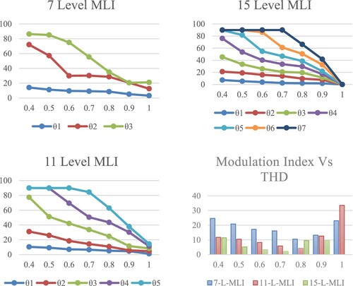
Figure 6. Total harmonic estimates and relatively closer optimal degrees determined with MNSGA-II for 7-, eleven-, and fifteen-level inverters.

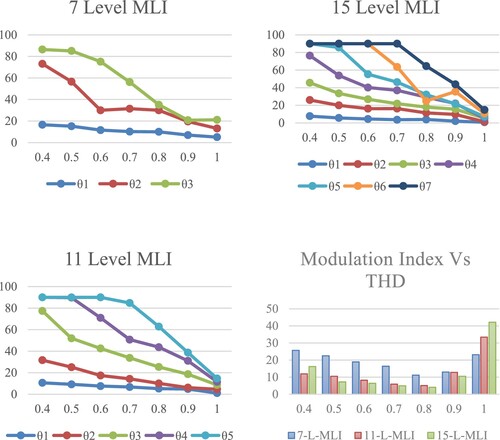
Conversely, Figures 6–8 demonstrate the approximately optimum switching degrees found utilizing MNSGA-II, PSO, and GA for 7-level, eleven-level, and fifteen-level multilevel inverters. Four figures show that the standard errors of switching angles determined utilizing MNSGA-II, PSO, GA, and SSA were completely different across 7- and 11-level multilevel inverters. The variance of a simulated result of fifteen-level multilevel inverters derived using SSA, on the other hand, is higher than those found with MNSGA-II, PSO, and GA. However, there seems to be no statistical difference in the mean difference produced via MNSGA-II, PSO, and GA.

Figure 7. PSO yields relatively closer angles for 7-, eleven-, and fifteen-level inverters, as well as total harmonic estimates.

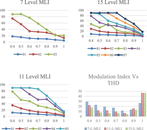
Figure 8. GA yields relatively closer angles for 7-, eleven-, and fifteen-level inverters, as well as total harmonic estimates.

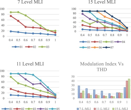
Consequently, optimum simulation findings predicated on MNSGA-II, PSO, and GA are more reliable. Figures 6–8 show the average Harmonic distortion estimates across four test setups. THDs estimated utilizing four approaches for 7- and 11-level multilevel inverters are pretty similar. That's not the case with fifteen-level multilevel inverters. When modulating indices are around 0.8 and 0.9, SSA yields more significant variance than MNSGA-II, PSO, and GA. The standard errors for residual modulation indices calculated utilizing four approaches varied somewhat.

Table 3 displays the average switching degrees achieved under modulation techniques indices with eleven-level multilevel inverters. According to the corresponding control strategies were achieved for modulated signal 0.8°, 6.57°, 18.94°, 27.18°, 45.14°, and 62.24°. Initially, for the identical modulation indexes, the corresponding switching angles were calculated by using the MNSGA-II method: 5.96°, 18.83°, 25.97°, 43.86°, and 61.64°. SSA estimated those numbers as 5.59°, 17.26°, 29.73°, 43.35°, and 62.98°, in that order. MNSGA-II discovered the following switching angles: 5.53°, 17.21°, 29.72°, 43.37°, and 62.99°. PSO computed those different control strategies as 5.58°, 17.25°, 29.72°, 43.37°, and 62.99°. THDs obtained via, MNSGA-II, SSA, MNSGA-II, PSO, and GA from all these five sets with alternative approaches were 6.8490%, 6.8698%, 6.1856%, 6.1860%, as well as 6.1901%, correspondingly. According to these data, SSA has a somewhat lower THD than MNSGA-II, GA, and PSO. This is because they provide worst Total harmonic distortion when utilizing PSO algorithms. PSO is a stochastic optimization technique and does not guarantee the best solution at the end of the search. It is possible for the particles to get stuck in a local optimum, meaning that the best solution was not found. This can result in a higher THD than expected.

A 15-level Multilevel inverter is created using MATLAB Simulink to validate further the findings and results of the simulation seen in Figures 9–12. Harmonic distortion ratios were therefore determined with m = 0.7 and m = 0.8 modulated indices utilizing switching angles discovered through using quantitative simulations of SSA shown in Table 4: For 0.7, 10.533, 35.546 as well as 72.350, as well as for 0.8, 9.803, 30.00 as well as 56.733. Figures 9 and 10 depict the stepped output voltages of 15-level multilevel inverters with two distinct modulation indexes and a nearly ideal switching pattern. Figures 11 and 12 demonstrate the THDs of such setups by using Fourier Evaluation Technique. The data shows that for m = 0.7 and m = 0.8, Harmonic distortion levels of 2.14% and 9.57% were attained.

Figure 9. Magnitudes of voltage measured at m = 0.8.

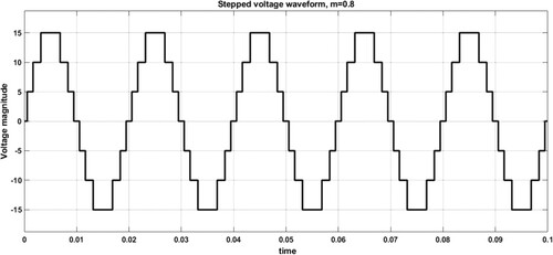
Figure 10. Magnitudes of voltage measured at m = 0.7.

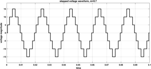
Figure 11. Using the simulation results, derived total harmonic values at m = 0.7.

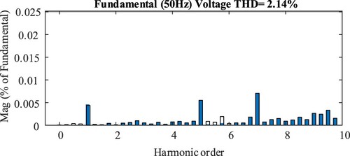
Figure 12. Using the simulation results, derived total harmonic findings at m = 0.8.

5.2. Hardware outcomes

The topological design, a culmination of the research efforts, is brought to fruition through a systematic prototyping process. This involves the meticulous assembly of components, adherence to established criteria, and the integration of cutting-edge specifications, as delineated in Table 5. The components’ grades and specific criteria, meticulously detailed in the preceding chapter, lay the foundation for the topological design that serves as the blueprint for the laboratory prototypes. Figure 13 in this study encapsulates the overarching schematic representation of our research, providing a visual guide to the conceptual framework guiding our investigations. This comprehensive schematic delineates the key components and interconnections within the intelligent power system developed, emphasizing the deployment of sustainable energy sources in conjunction with transmission and distribution systems networks. The representation extends to the critical utilization of cascaded H-bridge inverter topologies (MLIs) and power distribution operations, highlighting their significance for long-term power generation. Traditional models for selective harmonics reduction and the attainment of optimal switching frequencies in multilevel inverters are intricately interwoven into the depicted schematic, emphasizing the depth of our research focus.

Figure 13. Research's general schematic representation.

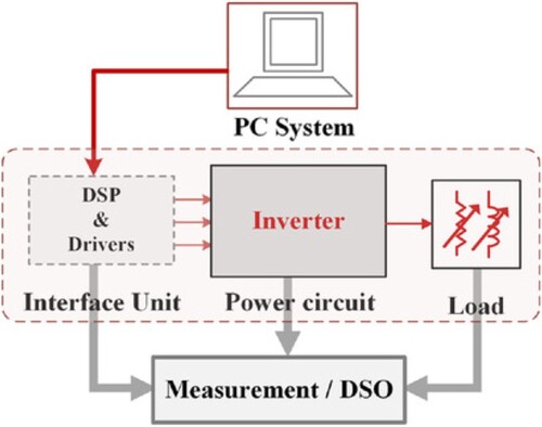
Table 5. Experimental testing specifications.

Component	Specifications
Switches	IGBT-FGA25N120
DC Supply	30 V and 60 V
Capacitors	110 V, 2400 μF
Microcontroller	TMS320F28378D, 250 MHz
Driver IC	TLP 258
Load (R)	100 Ω and 50 Ω
Load (RL)	100 Ω, 80 mH

Moving beyond the theoretical framework, Figure 14 offers a glimpse into the tangible aspects of our research – the Experimental Setup for laboratory investigations. This figure provides a visual insight into the real-world implementation of our proposed methodologies. The experimental setup is designed to validate and substantiate the theoretical constructs presented in the schematic representation (Figure 13). It encompasses the physical arrangement and connections of the multilevel inverters, the integration of renewable energy sources, and the implementation of the adaptive optimization techniques – MNSGA-II and salp swarm.

Figure 14. Experimental setup for laboratory investigations.

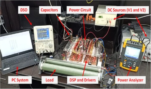
Table 5 further complements our experimental endeavours by presenting the Experimental Testing Specifications. This table provides a detailed overview of the parameters and conditions under which our experiments were conducted, ensuring transparency and replicability of our research. The specifications encompass various aspects, including the configurations of the multilevel inverters (seven-level, eleven-level, and fifteen-level MLIs), the modulation indices explored, and the specific conditions that were varied to assess the reliability and convergence rate of simulated data.

The process of topology design is a critical aspect of our study, involving a meticulous analysis of the architecture concerning supply voltages, current stress, and extreme temperature conditions. This analysis serves as the foundation for designing system elements that can effectively meet the demands of the intended application.

In our architecture, the switching component employed is the IGBT type FGA25N120, selected for its voltage and current ratings of 1200 V and 50 A, respectively. While these specifications may appear to surpass the immediate requirements, this intentional selection is made to ensure robust performance and longevity under varying operating conditions.

The capacitors, another crucial element in the design, are chosen based on the total discharge time limitation. Through a comprehensive design technique, capacitors with a capacity of 2400 F and a voltage rating of 110 V are selected. This careful consideration ensures that the capacitors align with the specific requirements of the system, contributing to optimal functionality.

The microcontroller at the heart of our architecture is the TMS320F28378D from Texas Instruments, boasting an impressive frequency management capability of up to 200 MHz. While this frequency range may seem excessive for the immediate task at hand, this deliberate choice is made to accommodate potential scalability and future enhancements, ensuring the system's adaptability.

To operate gate drivers, the TLP 258 is employed, featuring a maximum operating frequency of 28 kHz. This selection, in conjunction with the microcontroller's increased frequency, facilitates smooth operation and efficient control of the system. Different scenarios are explored under static and dynamic conditions, as showcased in Figures 15 and 16, demonstrating unit testing with continuous R and RL loads.

Figure 15. Voltage and current for constant R load.

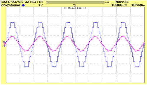
Figure 16. Voltage and current for constant RL load.

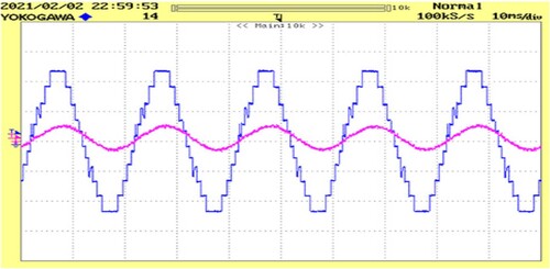
Dynamic situations, illustrated in Figure 17, simulate variations in the load, akin to a fan's capacity with regulation. The transition in load is clearly depicted, revealing a clean and glitch-free modulated signal as the resistor is adjusted in steps. This dynamic responsiveness underscores the effective functioning of the system.

Figure 17. Voltage and current for changing R load.

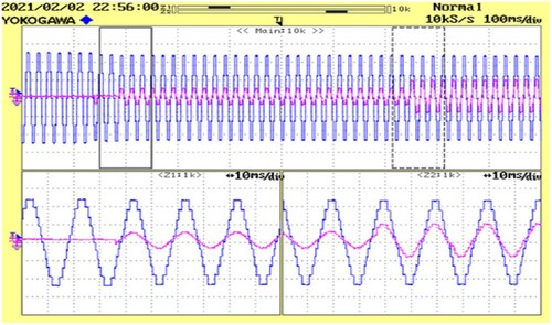
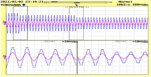
Figure 18 further elucidates the impact of adjusting the control signal. A noticeable correlation emerges between the reduction in switching frequency, the stages created in voltage levels, and the subsequent decrease in voltage amplitude. This dynamic behaviour showcases the system's adaptability and response to varying control signals.

Figure 18. Voltage and current for changing modulation index.

To quantify the effectiveness of the converters, PLECS technology is employed, considering the values obtained under the experimental settings. The calculated performance is an impressive 97.8%, affirming the efficiency of the system in converting input to desired output.

6. Conclusion

This paper concludes that by utilizing four intelligence optimization techniques, this work addresses the harmonics reduction issue for cascaded H-bridge multilevel inverters. Two of these techniques were introduced intelligence optimization algorithms: SSA and MNSGA-II. A much more common algorithm, GA and PSO, is built for comparison. Mathematical scenarios were simulated on seven-level, eleven-level, and fifteen-level multilevel inverters. For modulation indices varying between 0.4 and 1, optimal switching orientations were computed and presented using all approaches. Harmonic distortion results are indeed computed and shown. Mathematical computations reveal that the SSA and MNSGA-II algorithms solve the harmonics removal issue just as well as the GA and PSO algorithms. MNSGA-II, on the other hand, produces higher reliable mathematical simulations having lower standard deviation than SSA. Furthermore, a MATLAB Simulink model using a 7-level cascaded H-bridge Multilevel inverter is created to validate the modelling findings and voltages produced utilizing nearly optimal switching orientations in two example situations demonstrated. Harmonic distortion estimates for these situations were also determined using the FFT Analytical Model. It was discovered that perhaps the calculated values produced utilizing modelled scenarios and the MATLAB Simulink models produce identical results with a 1 percentage difference. The work would be expanded in the future by integrating multilevel inverters having uneven DC supplies to represent PV systems with varying outputs. Furthermore, hybridization of optimization approaches would be introduced to increase efficiency further.

Disclosure statement

No potential conflict of interest was reported by the author(s).

References

- Liu T, Li Y, Jiang L, et al. Multi-objective model predictive control of grid-connected three-level inverter based on hierarchical optimization. Chin J Elect Eng. 2021;7:64–72. doi:10.23919/CJEE.2021.000006
- Alamri B, Alharbi YM. A framework for optimum determination of LCL-filter parameters for N-level voltage source inverters using heuristic approach. IEEE Access. 2020;8:209212–209223. doi:10.1109/ACCESS.2020.3038583
- Iqbal A, Meraj M, Tariq M, et al. Experimental investigation and comparative evaluation of standard level shifted multi-carrier modulation schemes with a constraint GA based SHE techniques for a seven-level PUC inverter. IEEE Access. 2019;7:100605–100617. doi:10.1109/ACCESS.2019.2928693
- Re J, Li C, Jassal A, et al. Multi-domain design optimization of DV/DT filter for SiC-based three-phase inverters in high-frequency motor-drive applications. 2018 IEEE Energy Conversion Congress and Exposition, ECCE 2018, Portland, OR. 2018. p. 5215–5222. doi:10.1109/ECCE.2018.8557859
- Liu Z, Xia Z, Li D, et al. An optimal model predictive control method for five-level active NPC inverter. IEEE Access. 2020;8:221414–221423. doi:10.1109/ACCESS.2020.3043604
- Azurza Anderson J, Hanak EJ, Schrittwieser L, et al. All-silicon 99.35% efficient three-phase seven-level hybrid neutral point clamped/flying capacitor inverter. CPSS Trans Power Electron Appl. 2019;4:50–61. doi:10.24295/CPSSTPEA.2019.00006
- Nazer A, Driss S, Haddadi AM, et al. Optimal photovoltaic multi-string inverter topology selection based on reliability and cost analysis. IEEE Trans Sustain Energy. 2021;12:1186–1195. doi:10.1109/TSTE.2020.3038744
- Lopez-Lorente J, Liu XA, Best RJ, et al. Techno-economic assessment of grid-level battery energy storage supporting distributed photovoltaic power. IEEE Access. 2021;9:146256–146280. doi:10.1109/ACCESS.2021.3119436
- Manohar VJ, Trinad M, Ramana KV. Comparative analysis of NR and TBLO algorithms in control of cascaded MLI at low switching frequency. Procedia Comput Sci. 2016;85:976–986. doi:10.1016/J.PROCS.2016.05.290
- Yaqoob MT, Rahmat MK, Maharum SMM. Modified teaching learning based optimization for selective harmonic elimination in multilevel inverters. Ain Shams Eng J. 2022;13:101714. doi:10.1016/J.ASEJ.2022.101714
- Darvish Falehi A. Novel harmonic elimination strategy based on multi-objective grey wolf optimizer to ameliorate voltage quality of odd-nary multi-level structure. Heliyon. 2020;6:e03585. doi:10.1016/J.HELIYON.2020.E03585
- Barbie E, Baimel D, Kuperman A. Frequency spectra based approach to analytical formulation and minimization of voltage THD in staircase modulated multilevel inverters. Alexandria Eng J. 2022;61:7781–7809. doi:10.1016/J.AEJ.2022.01.031
- Sahoo B, Routray SK, Rout PK. Repetitive control and cascaded multilevel inverter with integrated hybrid active filter capability for wind energy conversion system. Eng Sci Technol Int J. 2019;22:811–826. doi:10.1016/J.JESTCH.2019.01.001
- Abdel-Mawgoud H, Ali A, Kamel S, et al. A modified manta ray foraging optimizer for planning inverter-based photovoltaic with battery energy storage system and wind turbine in distribution networks. IEEE Access. 2021;9:91062–91079. doi:10.1109/ACCESS.2021.3092145
- Fathy A, Kaaniche K, Alanazi TM. Recent approach based social spider optimizer for optimal sizing of hybrid PV/wind/battery/diesel integrated microgrid in Aljouf region. IEEE Access. 2020;8:57630–57645. doi:10.1109/ACCESS.2020.2982805
- Kamaraja AS, Priyadharshini K. Solar-powered multilevel inverter with a reduced number of switches. Int J Sci Technol Res. 2019;8:1545–1550.
- Hossain MI, Abido MA. Positive-negative sequence current controller for LVRT improvement of wind farms integrated MMC-HVDC network. IEEE Access. 2020;8:193314–193339. doi:10.1109/ACCESS.2020.3032400
- Trabelsi M, Vahedi H, Abu-Rub H. Review on single-DC-source multilevel inverters: topologies, challenges, industrial applications, and recommendations. IEEE Open J Ind Electron Soc. 2021;2:112–127. doi:10.1109/OJIES.2021.3054666
- Memon MA, Siddique MD, Saad M, et al. Asynchronous particle swarm optimization-genetic algorithm (APSO-GA) based selective harmonic elimination in a cascaded H-bridge multilevel inverter. IEEE Trans Ind Electron. 2021;69:1477–1487. doi:10.1109/TIE.2021.3060645
- Vasuki G, Vinothini M, Rushmithaa SB, et al. 13-level inverter configuration with a reduced auxiliary circuit for renewable energy applications. Proceedings of the 5th International Conference on Electronics, Communication and Aerospace Technology, ICECA 2021, Coimbatore. 2021. p. 101–105. doi:10.1109/ICECA52323.2021.9675929
- Siddique MD, Mekhilef S, Shah NM, et al. Low switching frequency based asymmetrical multilevel inverter topology with reduced switch count. IEEE Access. 2019;7:86374–86383. doi:10.1109/ACCESS.2019.2925277
- Kumar KK, Vaz FAJ, Iruthayarajan MW, et al. An automatic solar panel performance monitoring system and load control using IoT technique. 2023 5th International Conference on Smart Systems and Inventive Technology (ICSSIT), Tirunelveli, India. 2023. p. 8–12. doi:10.1109/ICSSIT55814.2023.10060886
- Anitha P, Kumar KK, Kamaraja AS. An improved design and performance enhancement of Y-source DC-DC boost combined phase shifted full bridge converter for electric vehicle battery charging applications. J Electr Eng Technol. 2023;18:2983–2996. doi:10.1007/S42835-023-01414-1/METRICS
- Islam J, Meraj ST, Masaoud A, et al. Opposition-based quantum bat algorithm to eliminate lower-order harmonics of multilevel inverters. IEEE Access. 2021;9:103610–103626. doi:10.1109/ACCESS.2021.3098190
- Routray A, Singh RK, Mahanty R. Harmonic minimization in three-phase hybrid cascaded multilevel inverter using modified particle swarm optimization. IEEE Trans Industr Inform. 2019;15:4407–4417. doi:10.1109/TII.2018.2883050
- Peng Y, Li Y, Lee KY, et al. Coordinated control strategy of PMSG and cascaded H-bridge STATCOM in dispersed wind farm for suppressing unbalanced grid voltage. IEEE Trans Sustain Energy. 2021;12:349–359. doi:10.1109/TSTE.2020.2995457
- Khomfoi S, Tolbert LM. Multilevel power converters. In: Butterworth Heinemann, editor. Power electronics handbook. Elsevier; 2011. p. 455–486. doi:10.1016/B978-0-12-382036-5.00017-3.
- Khamees AK, Abdelaziz AY, Eskaros MR, et al. Stochastic modeling for wind energy and multi-objective optimal power flow by novel meta-heuristic method. IEEE Access. 2021;9:158353–158366. doi:10.1109/ACCESS.2021.3127940
- Mirjalili S. Genetic algorithm. In: Evolutionary algorithms and neural networks. Studies in computational intelligence, Vol. 780. Cham: Springer; 2019. p. 43–55. doi:10.1007/978-3-319-93025-1_4/COVER.
- Kennedy J, Eberhart R. Particle swarm optimization. Proceedings of ICNN’95 – International Conference on Neural Networks, Perth. Vol. 4. 1995. p. 1942–1948. doi:10.1109/ICNN.1995.488968
- Mirjalili S, Gandomi AH, Mirjalili SZ, et al. Salp swarm algorithm: a bio-inspired optimizer for engineering design problems. Adv Eng Softw. 2017;114:163–191. doi:10.1016/J.ADVENGSOFT.2017.07.002