A Practical Guide to Power Analyses of Moderation Effects in Multisite Individual and Cluster Randomized Trials

Abstract

Multisite trials that randomize individuals (e.g., students) within sites (e.g., schools) or clusters (e.g., teachers/classrooms) within sites (e.g., schools) are commonly used for program evaluation because they provide opportunities to learn about treatment effects as well as their heterogeneity across sites and subgroups (defined by moderating variables). Despite the rich opportunities they present, a critical step in ensuring those opportunities is identifying the sample size that provides sufficient power to detect the desired effects if they exist. Although a strong literature base for conducting power analyses for the moderator effects in multisite trials already exists, software for power analysis of moderator effects is not readily available in an accessible platform. The purpose of this tutorial paper is to provide practical guidance on implementing power analyses of moderator effects in multisite individual and cluster randomized trials. We conceptually motivate, describe, and demonstrate the calculation of statistical power and minimum detectable effect size difference (MDESD) using highly accessible software. We conclude by outlining guidelines on power analysis of moderator effects in multisite individual randomized trials (MIRTs) and multisite cluster randomized trials (MCRTs).

Keywords:

• Minimum detectable effect size difference (MDESD)
• moderator
• multisite cluster randomized trials (MCRTs)
• multisite individual randomized trials (MIRTs)
• statistical power

Introduction

Recently literature has emphasized the critical role of moving beyond designing studies that answer the “what works” question, or to detect the main/average treatment effect, to designing studies to answer “for whom and under what conditions a treatment is most effective” or to detect treatment effect heterogeneity (interaction effects or moderator effects, e.g., US DoE & NSF, 2013; Weiss et al., 2014). For example, an important line of inquiry in many studies examines how treatment effects vary by different characteristics of students (e.g., race and pretest), teachers (e.g., gender and teaching experience), and schools (e.g., urbanity and size). These types of “for whom, and under what circumstances” questions are fundamental for understanding treatment effect variation and the potential for scaling a program to a wide range of schools and students.

Cluster randomized trials (CRTs) and multisite randomized trials (MRTs) are among the most common designs used in education research to probe these types of complementary effects (e.g., Spybrook et al., 2016; Spybrook & Raudenbush, 2009). CRTs are defined by random assignment of the top level of clusters into the treatment or control condition. CRTs include, for example, two-level designs that randomly assign schools (level 2) (including students or level 1) while three-level CRTs randomly assign schools (level 3) including the teachers/classrooms (level 2) within each school and students (level 1) within each teacher within each school. In contrast, MRTs involve randomly assigning the sublevel of clusters into the treatment and control groups. MRTs include, for example, multisite individual randomized trials (MIRTs) that randomly assign individuals (e.g., students) within sites (e.g., schools) and multisite cluster randomized trials (MCRTs) that randomly assign intermediate clusters (e.g., teachers/classrooms) including the students within each teacher/classroom within sites (e.g., schools).

In planning CRTs and MRTs to detect main or moderator effects, a critical step is identifying a sample size that provides sufficient power to detect a desired effect if it exists. Power analyses are now routinely required by grant agencies and form a key basis for the requisite scale of most experimental studies (e.g., US DoE & NSF, 2013; Kelcey et al., 2019). A strong literature base for conducting power analyses for moderator effects in CRTs and MRTs has been developed over recent decades. For example, the statistical methods and software have been developed for power analysis of moderator effects for binary and continuous moderators at different levels in two- and three-level CRTs (Dong et al., 2018, 2021b; Spybrook et al., 2016). Regarding MRTs, Raudenbush and Liu (2000) developed power formulas for the site-level (level-2) binary moderator effect in MRTs, and Bloom and Spybrook (2017) developed formulas for the minimum detectable effect size difference (MDESD) for the site-level binary moderator in MRTs and MCRTs. Dong et al. (2021a, 2023a) further developed a comprehensive statistical framework for power analysis of moderator effects in two-level MIRTs and three-level MCRTs. In addition, Dong et al. (2023c) created a Microsoft Excel-based software “PowerUp!-Moderator-MRTs” (https://tinyurl.com/327tvufc), which is the only software for power analysis of moderator effects in MRTs to our knowledge.

This framework considers the intersections of three key facets of multilevel moderation that are common in practice: (a) level of the moderator (e.g., student-, classroom- or school-level), (b) effects of treatment and/or moderation (i.e., (non)randomly varying slopes (coefficients) for the treatment variable and/or the treatment-by-moderator interaction term), and (c) moderator scale (e.g., categorical, continuous). Despite the recent technical developments of analyses across these facets, guidance detailing the practical use and implementation of these calculations in software for MIRTs and MCRTs is lacking.

The purpose of this tutorial paper is to provide practical guidance on conducting power analyses of moderator effects in MCRTs and MIRTs across the three facets outlined above. The paper is organized as follows. First, we outline an illustrative example to be used throughout our paper. Second, we discuss the design options and introduce the software modules implementing the calculations. Third, we demonstrate the calculation of statistical power and MDESD using the software. Fourth, we compare features and considerations of the power and MDESD analyses across main and moderation effects and summarize our findings. Finally, we conclude by offering suggestions on conducting power analysis of moderator effects in MRTs.

An illustrative example for investigating moderator effects in MRTs

Consider an evaluation of the effects of a teacher professional development program on student outcomes. Assume teachers within schools are randomly assigned to receive professional development (treatment) or business as usual (control). Under this scenario, we may adopt a three-level MCRT with students nested within teachers (clusters) and teachers nested within schools (sites). To facilitate discussion, we use the same figure in Dong et al. (2023a, Figure 1) to illustrate the simplified conceptual framework for investigating moderation effects of the professional development on student outcomes in three-level MCRTs in Figure 1.

Figure 1. A conceptual framework for investigating moderation effects of professional development.

Note: This figure is a reproduction of Figure 1 from Dong et al. (2023a).

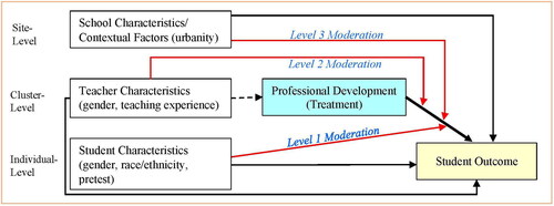
In this hypothetical study, we can conceptually describe the study as a multi-school teacher randomized design with a three-level hierarchy: students as level one (individuals), teachers/classrooms as level two (clusters), and schools as level three (sites). In this MCRT, we assign the treatment (teacher professional development) at the teacher level or level two. Likewise, our design uses schools as sites (or blocks) such that both treatment and control conditions exist within each school. The random assignment of the treatment conditions to teachers renders treatment status independent of other teacher and classroom characteristics (dotted arrow in Figure); in non-experimental designs, teacher/classroom characteristics may be related to the treatment status (e.g., see Dong et al., 2023b). Similarly, under random assignment, the characteristics of students, teachers, and schools may be related to the student outcome (black arrows); however, such relationships will not affect the accuracy of the main effect estimates of the professional development (or moderation effects) but may affect the precision (e.g., standard error, power) of the effect estimates. Finally, the effects of professional development on student outcome may differ by the characteristics of students, teachers, and schools (red arrows). Note that it is also common to complement moderation analyses by probing the mediation effect. For instance, prior literature has investigated how the effect of the teacher professional development on student achievement is mediated by teacher knowledge or instruction (Kelcey et al., 2019, 2020); however, in our analysis here we focus specifically on moderation effects.

In a second hypothetical example, we might consider a study that examines teacher outcomes (e.g., teacher knowledge or instruction) only. In this setting, we would eliminate the student-level entirely such that the design reduces to a simpler two-level MIRT (i.e., teachers randomly assigned within schools). In turn, we can investigate moderation effects of the characteristics of teachers (now the individual-level or level 1) and schools (now the site-level or level 2) on teacher outcomes (Kelcey et al., 2017).

Design options and software modules

In the illustrative example outlined above, we have various options to investigate moderator effects in both three-level MCRTs and two-level MIRTs. The two- and three-level hierarchical linear models for the moderation analysis, using the notation of Raudenbush and Bryk (2002), are summarized in Table 1. In these models, the outcome variable is $Y,$ and the covariates are $X$ at level 1 and $W$ at level 2. The treatment variables are $T_{\mathit{\text{ij}}}$ and $T_{\mathit{\text{jk}}}$ for two- and three-level models, respectively. The variables, $M_{\mathit{\text{ij}}}^{(1)}$ and $M_j^{(2)},$ indicate level-1 and level-2 moderators in two-level models, respectively; The variables, $M_{\mathit{\text{ijk}}}^{(1)},$ $M_{\mathit{\text{jk}}}^{(2)},$ and $M_k^{(3)}$ indicate level-1, -2, and -3 moderators in three-level models, respectively.

Table 1. Summary of statistical models for the moderation analysis in two-level MIRTs and three-level MCRTs.

Model number	Statistical model
MRT2-1R-1	L1: $Y_{\mathit{\text{ij}}}={\beta }_{0j}+{\beta }_{1j}{T}_{\mathit{\text{ij}}}+{\beta }_{2j}{T}_{\mathit{\text{ij}}}{M}_{\mathit{\text{ij}}}^{(1)}+{\beta }_{3j}{M}_{\mathit{\text{ij}}}^{(1)}+{\beta }_{4j}{X}_{\mathit{\text{ij}}}+r_{\mathit{\text{ij}}}$	$r_{\mathit{\text{ij}}}\sim N(0,{\sigma }_{|T,M,X}^2)$
	L2: ${\beta }_{0j}={\gamma }_{00}+u_{0j}$ ${\beta }_{1j}={\gamma }_{10}+u_{1j}$ ${\beta }_{2j}={\gamma }_{20}+u_{2j}$ ${\beta }_{3j}={\gamma }_{30}$ ${\beta }_{4j}={\gamma }_{40}$	$\left(\begin{array}{c}{u}_{0j}\\ u_{1j}\\ u_{2j}\end{array}\right)$∼$N\left[\left(\begin{array}{c}0\\ 0\\ 0\end{array}\right),\left(\begin{array}{ccc}{\tau }_{00}^2& {\tau }_{01}^{}& {\tau }_{02}^{}\\ & {\tau }_{11}^2& {\tau }_{12}^{}\\ & & {\tau }_{22}^2\end{array}\right)\right]$
MRT2-1R-2	L1: $Y_{\mathit{\text{ij}}}={\beta }_{0j}+{\beta }_{1j}{T}_{\mathit{\text{ij}}}+{\beta }_{2j}{X}_{\mathit{\text{ij}}}+r_{\mathit{\text{ij}}}$	$r_{\mathit{\text{ij}}}\sim N(0,{\sigma }_{|T,M,X}^2)$
	L2: ${\beta }_{0j}={\gamma }_{00}+{\gamma }_{01}{M}_j^{\left(2\right)}+u_{0j}$ ${\beta }_{1j}={\gamma }_{10}+{\gamma }_{11}{M}_j^{\left(2\right)}+u_{1j}$ ${\beta }_{2j}={\gamma }_{20}$	$\left(\begin{array}{c}{u}_{0j}\\ u_{1j}\end{array}\right)$∼$N\left[\left(\begin{array}{c}0\\ 0\end{array}\right),\left(\begin{array}{cc}{\tau }_{00|M}^2& {\tau }_{01|M}^{}\\ & {\tau }_{11|M}^2\end{array}\right)\right]$
MRT2-1N-1	L1: $Y_{\mathit{\text{ij}}}={\beta }_{0j}+{\beta }_{1j}{T}_{\mathit{\text{ij}}}+{\beta }_{2j}{T}_{\mathit{\text{ij}}}{M}_{\mathit{\text{ij}}}^{(1)}+{\beta }_{3j}{M}_{\mathit{\text{ij}}}^{(1)}+{\beta }_{4j}{X}_{\mathit{\text{ij}}}+r_{\mathit{\text{ij}}}$	$r_{\mathit{\text{ij}}}\sim N(0,{\sigma }_{|T,M,X}^2)$
	L2: ${\beta }_{0j}={\gamma }_{00}+u_{0j}$ ${\beta }_{1j}={\gamma }_{10}$ ${\beta }_{2j}={\gamma }_{20}$ ${\beta }_{3j}={\gamma }_{30}$ ${\beta }_{4j}={\gamma }_{40}$	$u_{0j}\sim N(0,{\tau }_{00}^2)$
MRT2-1N-2	L1: $Y_{\mathit{\text{ij}}}={\beta }_{0j}+{\beta }_{1j}{T}_{\mathit{\text{ij}}}+{\beta }_{2j}{X}_{\mathit{\text{ij}}}+r_{\mathit{\text{ij}}}$	$r_{\mathit{\text{ij}}}\sim N(0,{\sigma }_{|T,M,X}^2)$
	L2: ${\beta }_{0j}={\gamma }_{00}+{\gamma }_{01}{M}_j^{\left(2\right)}+u_{0j}$ ${\beta }_{1j}={\gamma }_{10}+{\gamma }_{11}{M}_j^{\left(2\right)}$ ${\beta }_{2j}={\gamma }_{20}$	$u_{0j}\sim N(0,{\tau }_{00}^2)$
MRT3-2R-1	L1: $Y_{\mathit{\text{ijk}}}={\pi }_{0\mathit{\text{jk}}}+{\pi }_{1\mathit{\text{jk}}}{M}_{\mathit{\text{ijk}}}^{(1)}+{\pi }_{2\mathit{\text{jk}}}{X}_{\mathit{\text{ijk}}}+e_{\mathit{\text{ijk}}}$	$e_{\mathit{\text{ijk}}}\sim N(0,{\sigma }_{1|M,X}^2)$
	L2: ${\pi }_{0\mathit{\text{jk}}}={\beta }_{00k}+{\beta }_{01k}{T}_{\mathit{\text{jk}}}+{\beta }_{02k}{W}_{\mathit{\text{jk}}}+r_{0\mathit{\text{jk}}}$ ${\pi }_{1\mathit{\text{jk}}}={\beta }_{10k}+{\beta }_{11k}{T}_{\mathit{\text{jk}}}+r_{1\mathit{\text{jk}}}$ ${\pi }_{2\mathit{\text{jk}}}={\beta }_{20k}$	$\left(\begin{array}{c}{r}_{0\mathit{\text{jk}}}\\ r_{1\mathit{\text{jk}}}\end{array}\right)\sim N\left[\left(\begin{array}{c}0\\ 0\end{array}\right),\left(\begin{array}{cc}{\tau }_{00|T,W}^2& {\tau }_{01|T,W}\\ & {\tau }_{11|T}^2\end{array}\right)\right]$
	L3: ${\beta }_{00k}={\gamma }_{000}+u_{00k}$ ${\beta }_{01k}={\gamma }_{010}+u_{01k}$ ${\beta }_{02k}={\gamma }_{020}$ ${\beta }_{10k}={\gamma }_{100}+u_{10k}$ ${\beta }_{11k}={\gamma }_{110}+u_{11k}$ ${\beta }_{20k}={\gamma }_{200}$	$\left(\begin{array}{c}\begin{array}{c}{u}_{00k}\\ u_{01k}\\ u_{10k}\end{array}\\ u_{11k}\end{array}\right)\sim N\left[\left(\begin{array}{c}\begin{array}{c}0\\ 0\\ 0\end{array}\\ 0\end{array}\right),\left(\begin{array}{cccc}{\tau }_{0000}^2& {\tau }_{0001}& {\tau }_{0010}& {\tau }_{0011}\\ & {\tau }_{0101}^2& {\tau }_{0110}& {\tau }_{0111}\\ & & {\tau }_{1010}^2& {\tau }_{1011}\\ & & & {\tau }_{1111}^2\end{array}\right)\right]$
MRT3-2R-2	L1: $Y_{\mathit{\text{ijk}}}={\pi }_{0\mathit{\text{jk}}}+{\pi }_{1\mathit{\text{jk}}}{X}_{\mathit{\text{ijk}}}+e_{\mathit{\text{ijk}}},$	$e_{\mathit{\text{ijk}}}\sim N(0,{\sigma }_{1|X}^2)$
	L2: ${\pi }_{0\mathit{\text{jk}}}={\beta }_{00k}+{\beta }_{01k}{T}_{\mathit{\text{jk}}}+{\beta }_{02k}{T}_{\mathit{\text{jk}}}{M}_{\mathit{\text{jk}}}^{(2)}+{\beta }_{03k}{M}_{\mathit{\text{jk}}}^{(2)}+{\beta }_{04k}{W}_{\mathit{\text{jk}}}+r_{0\mathit{\text{jk}}}$ ${\pi }_{1\mathit{\text{jk}}}={\beta }_{10k}$	$r_{0\mathit{\text{jk}}}\sim N(0,{\tau }_{00|T,M,W}^2$)
	L3: ${\beta }_{00k}={\gamma }_{000}+u_{00k}$ ${\beta }_{01k}={\gamma }_{010}+u_{01k}$ ${\beta }_{02k}={\gamma }_{020}+u_{02k}$ ${\beta }_{03k}={\gamma }_{030}$ ${\beta }_{04k}={\gamma }_{040}$ ${\beta }_{10k}={\gamma }_{100}$	$\left(\begin{array}{c}{u}_{00k}\\ u_{01k}\\ u_{02k}\end{array}\right)\sim N\left[\left(\begin{array}{c}0\\ 0\\ 0\end{array}\right),\left(\begin{array}{ccc}{\tau }_{0000}^2& {\tau }_{0001}& {\tau }_{0002}\\ & {\tau }_{0101}^2& {\tau }_{0102}\\ & & {\tau }_{0202}^2\end{array}\right)\right]$
MRT3-2R-3	L1: $Y_{\mathit{\text{ijk}}}={\pi }_{0\mathit{\text{jk}}}+{\pi }_{1\mathit{\text{jk}}}{X}_{\mathit{\text{ijk}}}+e_{\mathit{\text{ijk}}}$	$e_{\mathit{\text{ijk}}}\sim N(0,{\sigma }_{1|X}^2)$
	L2: ${\pi }_{0\mathit{\text{jk}}}={\beta }_{00k}+{\beta }_{01k}{T}_{\mathit{\text{jk}}}+{\beta }_{02k}{W}_{\mathit{\text{jk}}}+r_{0\mathit{\text{jk}}}$ ${\pi }_{1\mathit{\text{jk}}}={\beta }_{10k}$	$r_{0\mathit{\text{jk}}}\sim N(0,{\tau }_{00|T,W}^2$)
	L3: ${\beta }_{00k}={\gamma }_{000}+{\gamma }_{001}{M}_k^{\left(3\right)}+u_{00k}$ ${\beta }_{01k}={\gamma }_{010}+{\gamma }_{011}{M}_k^{\left(3\right)}+u_{01k}$ ${\beta }_{02k}={\gamma }_{020}$ ${\beta }_{10k}={\gamma }_{100}$	$\left(\begin{array}{c}{u}_{00k}\\ u_{01k}\end{array}\right)\sim N\left[\left(\begin{array}{c}0\\ 0\end{array}\right),\left(\begin{array}{cc}{\tau }_{0000|M}^2& {\tau }_{0001|M}\\ & {\tau }_{0101|M}^2\end{array}\right)\right]$
MRT3-2N-1	L1: $Y_{\mathit{\text{ijk}}}={\pi }_{0\mathit{\text{jk}}}+{\pi }_{1\mathit{\text{jk}}}{M}_{\mathit{\text{ijk}}}^{(1)}+{\pi }_{2\mathit{\text{jk}}}{X}_{\mathit{\text{ijk}}}+e_{\mathit{\text{ijk}}}$	$e_{\mathit{\text{ijk}}}\sim N(0,{\sigma }_{1|M,X}^2)$
	L2: ${\pi }_{0\mathit{\text{jk}}}={\beta }_{00k}+{\beta }_{01k}{T}_{\mathit{\text{jk}}}+{\beta }_{02k}{W}_{\mathit{\text{jk}}}+r_{0\mathit{\text{jk}}}$ ${\pi }_{1\mathit{\text{jk}}}={\beta }_{10k}+{\beta }_{11k}{T}_{\mathit{\text{jk}}}$ ${\pi }_{2\mathit{\text{jk}}}={\beta }_{20k}$	$r_{0\mathit{\text{jk}}}\sim N(0,{\tau }_{00|T,W}^2)$
	L3: ${\beta }_{00k}={\gamma }_{000}+u_{00k}$ ${\beta }_{01k}={\gamma }_{010}$ ${\beta }_{02k}={\gamma }_{020}$ ${\beta }_{10k}={\gamma }_{100}$ ${\beta }_{11k}={\gamma }_{110}$ ${\beta }_{20k}={\gamma }_{200}$	$u_{00k}\sim N(0,{\tau }_{0000}^2)$
MRT3-2N-2	L1: $Y_{\mathit{\text{ijk}}}={\pi }_{0\mathit{\text{jk}}}+{\pi }_{1\mathit{\text{jk}}}{X}_{\mathit{\text{ijk}}}+e_{\mathit{\text{ijk}}}$	$e_{\mathit{\text{ijk}}}\sim N(0,{\sigma }_{1|X}^2)$
	L2: ${\pi }_{0\mathit{\text{jk}}}={\beta }_{00k}+{\beta }_{01k}{T}_{\mathit{\text{jk}}}+{\beta }_{02k}{T}_{\mathit{\text{jk}}}{M}_{\mathit{\text{jk}}}^{(2)}+{\beta }_{03k}{M}_{\mathit{\text{jk}}}^{(2)}+{\beta }_{04k}{W}_{\mathit{\text{jk}}}+r_{0\mathit{\text{jk}}}$ ${\pi }_{1\mathit{\text{jk}}}={\beta }_{10k}$	$r_{0\mathit{\text{jk}}}\sim N(0,{\tau }_{00|T,M,W}^2$)
	L3: ${\beta }_{00k}={\gamma }_{000}+u_{00k}$ ${\beta }_{01k}={\gamma }_{010}$ ${\beta }_{02k}={\gamma }_{020}$ ${\beta }_{03k}={\gamma }_{030}$ ${\beta }_{04k}={\gamma }_{040}$ ${\beta }_{10k}={\gamma }_{100}$	$u_{00k}\sim N(0,{\tau }_{0000}^2)$
MRT3-2N-3	L1: $Y_{\mathit{\text{ijk}}}={\pi }_{0\mathit{\text{jk}}}+{\pi }_{1\mathit{\text{jk}}}{X}_{\mathit{\text{ijk}}}+e_{\mathit{\text{ijk}}}$	$e_{\mathit{\text{ijk}}}\sim N(0,{\sigma }_{1|X}^2)$
	L2: ${\pi }_{0\mathit{\text{jk}}}={\beta }_{00k}+{\beta }_{01k}{T}_{\mathit{\text{jk}}}+{\beta }_{02k}{W}_{\mathit{\text{jk}}}+r_{0\mathit{\text{jk}}}$ ${\pi }_{1\mathit{\text{jk}}}={\beta }_{10k}$	$r_{0\mathit{\text{jk}}}\sim N(0,{\tau }_{00|T,W}^2$)
	L3: ${\beta }_{00k}={\gamma }_{000}+{\gamma }_{001}{M}_k^{\left(3\right)}+u_{00k}$ ${\beta }_{01k}={\gamma }_{010}+{\gamma }_{011}{M}_k^{\left(3\right)}$ ${\beta }_{02k}={\gamma }_{020}$ ${\beta }_{10k}={\gamma }_{100}$	$u_{00k}\sim N(0,{\tau }_{0000|M}^2)$

Note. MRT2-1R-1 and MRT2-1R-2 stand for two-level MRTs with a level-1 and a level-2 moderator with random slopes, respectively. MRT2-1N-1 and MRT2-1N-2 stand for two-level MRTs with a level-1 and a level-2 moderator with nonrandomly varying slopes, respectively. MRT3-2R-1, MRT3-2R-2, and MRT3-2R-3 stand for three-level MRTs where treatment is at level 2 with a level-1, -2, -3 moderator with random slopes, respectively. MRT3-2N-1, MRT3-2N-2, and MRT3-2N-3 stand for three-level MCRTs where treatment is at level 2 with a level-1, -2, -3 moderator with nonrandomly varying slopes, respectively.

For two-level models, parameters ${\gamma }_{20}$ and ${\gamma }_{11}$ represent the average moderator effects for level-1 and level-2 moderators, respectively; ${\tau }_{22}^2$ represents the variance of the moderator effect of level-1 moderator across sites for the random slope model (MRT2-1R-1). ${\tau }_{11|M}^2$ represents the treatment effect variation across sites conditional on the level-2 moderator. For three-level models, parameters ${\gamma }_{110},$ ${\gamma }_{020},$ and ${\gamma }_{011}$ represent the average moderator effects for level-1, -2, and -3 moderators, respectively; ${\tau }_{1111}^2$ and ${\tau }_{0202}^2$ represent the variance of the moderator effect of level-1 and -2 moderators across sites for the random slope model (MRT3-2R-1 and MRT3-2R-2), respectively. ${\tau }_{0101|M}^2$ represents the treatment effect variation across sites conditional on the level-3 moderator.

Table 2 presents the list of design options and software modules in PowerUp!-Moderator-MRTs.

Table 2. List of design options and software modules.

1	2	3	4	5	6	7	8	9
Number of total levels of clustering	Model number	Level of treatment	Level of moderator	Slope of treatment or moderation	Binary moderator		Continuous moderator
					MDESD calculation	Power calculation	MDESD calculation	Power calculation
2	MRT2-1R-1	1	1	Random	MRT21R_MDESD	MRT21R_Power	MRT21Rc_MDESD	MRT21Rc_Power
	MRT2-1R-2	1	2	Random
	MRT2-1N-1	1	1	Nonrandomly Varying	MRT21N_MDESD	MRT21N_Power	MRT21Nc_MDESD	MRT21Nc_Power
	MRT2-1N-2	1	2	Nonrandomly Varying
3	MRT3-2R-1	2	1	Random	MRT32R_MDESD	MRT32R_Power	MRT32Rc_MDESD	MRT32Rc_Power
	MRT3-2R-2	2	2	Random
	MRT3-2R-3	2	3	Random
	MRT3-2N-1	2	1	Nonrandomly Varying	MRT32N_MDESD	MRT32N_Power	MRT32Nc_MDESD	MRT32Nc_Power
	MRT3-2N-2	2	2	Nonrandomly Varying
	MRT3-2N-3	2	3	Nonrandomly Varying

Researchers first need to specify the hierarchic structure or the number of total levels of clustering in their study design (Column 1 in Table 2, e.g., selecting a two-level MIRT or three-level MCRT). Then researchers need to determine the statistical models for the moderator analysis (Column 2). The model numbers correspond to those in Table 1 and in Dong et al. (2021a, Table 1; 2023a, Table 2).

In what follows, we focus on a three-level MCRT using our first example above (Tables 1 and 2); however, a simpler two-level MIRT (e.g., using the second example above) follows the same conceptual procedures (see Dong et al., 2021a). Our example analyses draw on several different specifications. We first consider specifications that examine individual-level moderators (e.g., student variables). In this setting, we examine the Model MRT3-2R-1 framework that describes a three-level MCRT (Table 2, Column 1), with treatment at level 2 (Table 2, Column 3), moderator at level 1 (Table 2, Column 4), and random slopes for the moderation/interaction term across sites and the moderator variable across level 2 clusters (Table 2, Column 5). We then consider an alternative specification that adopts the Model MRT3-2N-1 framework that draws on a three-level MCRT (Table 2, Column 1), with treatment at level 2 (Table 2, Column 3), moderator at level 1 (Table 2, Column 4), and constant slope for the moderation term across sites and nonrandomly vary slope for the moderator variable across level 2 clusters (Table 2, Column 5). The primary difference between these two specifications is the introduction of random effects or variation of effects across clusters (level 2) and sites (level 3). Model MRT3-2R-1 allows the slope of level-1 moderator to interact with the treatment status (fixed effect interaction, ${\gamma }_{110}$) while also varying randomly across level-2 clusters ($r_{1\mathit{\text{jk}}}$) and level 3 sites ($u_{10k}$) and allowing the moderation effect to randomly vary across sites ($u_{11k}$). In contrast, Model MRT3-2N-1 allows the slope of level-1 moderator to vary only by the treatment status and therefore it does not randomly vary across level-2 clusters, and the moderation effect is constant across sites.

Second, we consider parallel specifications for examining teacher-level moderators using both the random (MRT3-2R-2) and nonrandom specifications (MRT3-2N-2). Model MRT3-2R-2 refers to a three-level MCRT (Table 2, Column 1), with treatment at level 2 (Table 2, Column 3), moderator at level 2 (Table 2, Column 4), and random slope for the moderation/interaction term across sites (Table 2, Column 5). Model MRT3-2N-2 takes up that same design but constrains the slope for the moderation/interaction term to be fixed across sites. In other words, the difference between Models MRT3-2R-2 and MRT3-2N-2 is that the treatment effect varies by the level-2 moderator and the moderation effect randomly varies across sites in MRT3-2R-2 while the treatment effect varies by the moderator but the moderation effect is constant across sites in MRT3-2N-2.

Third, we consider parallel specifications for examining school-level moderators. Model MRT3-2R-3 examines the random effect version and describes to a three-level MCRT (Table 2, Column 1), with treatment at level 2 (Table 2, Column 3), moderator at level 3 (Table 2, Column 4), and random slope for treatment across sites (Table 2, Column 5). In contrast, Model MRT3-2N-3 constrains those random effects and describes a three-level MCRT, with treatment at level 2, moderator at level 3, and nonrandomly varying slope for treatment across sites. Analogous to the previous sections, the difference between Models MRT3-2R-3 and MRT3-2N-3 is that the treatment effect does not only vary by the level-3 moderator but also randomly varies across sites in MRT3-2R-2 while the treatment effect only varies by the level-3 moderator and does not randomly vary across sites in MRT3-2N-3.

A priori selection of the scope of the random effect structure (e.g., random versus nonrandom slopes for the treatment/moderator/moderation) is a difficult issue because it necessarily needs to balance a number of competing criteria and as a result it has not been clearly resolved for the purposes of study planning (e.g., Bates et al., 2015). Some research has suggested adopting the maximal random effects structure allowable by design (e.g., allowing all or most slopes to randomly vary; Barr et al., 2013) because it best aligns with the design and provides is the most conservative honors the design and driven by design consideration only. However, competing research has also widely demonstrated that adopting a complex random effects structure (e.g., multiple random slopes) can quickly introduce estimation or convergence issues because complex structures are rarely empirically supported and often overparameterized or overfitted in practice (e.g., models are not supported by the data; Matuschek et al., 2017). More practical research has also developed less theoretical approaches and tools that attempt to balance minimal (e.g., no random slopes) versus maximal (e.g., all slopes are allowed to randomly vary) random effect structures by balancing the tradeoffs between, for example, power, type one error, program theory and/or empirical evidence from literature (e.g., Phelps et al., 2016; Seedorff et al., 2019). Still other approaches suggest that if there is no clear theory or prior studies suggesting nonrandomly varying slope models, it may be prudent to assume these slopes randomly vary because this typically produces conservative power estimates (Dong et al., 2021a).

In addition to determining the statistical models for moderator analysis, researchers need to determine whether the moderator is a binary or continuous variable. The definitions of effect sizes for a binary moderator and a continuous moderator are different (Dong et al., 2018, 2021a, 2021b, 2023a). The effect size for a binary moderator is the standardized treatment effect difference between two moderator subgroups; the effect size for a continuous moderator is the difference of the standardized regression coefficients for the moderator between the treatment and control groups, or the standardized treatment effect difference associated with one standard deviation change on the moderator variable.

Regarding power analysis, there are two options: (1) what is the power to detect a particular moderation effect size, and (2) what is the minimum detectable effect size difference (MDESD) given power of 0.80. The choice between these options depends on the unknown entity. Option (1) is most appropriate when the effect size of interest for the moderator effect is pre-determined. Option (2) is most appropriate when the effect size of interest for the moderator effect is not set. Columns 6 and 8 in Table 2 are the modules for the MDESD calculations for the binary moderator and continuous moderator, respectively; Columns 7 and 9 are the modules for the power calculations for the binary moderator and continuous moderator, respectively. Note that all levels of moderators with the same number of total levels of clustering and same type of slopes (random or nonrandomly varying) are grouped in the same modules. For example, Module MRT32R_MDESD is for the MDESD calculations for levels-1, 2, and 3 binary moderators in the random slope models; Module MRT32Nc_power is for the power calculations for levels-1, 2, and 3 continuous moderators in the nonrandomly varying slope models.

Demonstration

Three-level MCRTs

In this section, we demonstrate power analyses of moderation at all three levels in three-level MCRTs. Consider a team of researchers designing an MCRT to investigate the moderator effects of a professional development program in reducing students’ concentration problems in the illustrative example discussed above (Figure 1). They approach the power analyses of moderator effects from two perspectives: (1) what is the power for a meaningful moderation effect size and (2) what is the MDESD given power of 0.80. The team can conduct power analysis by following the steps below.

Step 1. Select the appropriate design and corresponding software module

The team can first click the button “Click to Choose Your Design from the List” on the main interface of the software. The team then needs to choose the corresponding software modules (Columns 6–9, Table 2) to calculate the MDESD or power based on the features of their study design (e.g., random or nonrandomly varying slope, binary or continuous moderator) as discussed in the design options and software module section above. Suppose the team would like to conduct power analysis of moderator effect for a binary moderator (either level-1, 2, or 3) with random slope. The team can choose Module MRT32R-MDESD for calculation of MDESD and Module MRT32R_Power for calculation of power. Clicking “MRT32R-MDESD” will lead to the spreadsheet like Figure 2; clicking “MRT32R-Power” will lead to the spreadsheet like Figure 3.

Figure 2. An example of MDESD calculation for binary moderators at level-1, -2, and -3 with random effects in three-level MCRT.

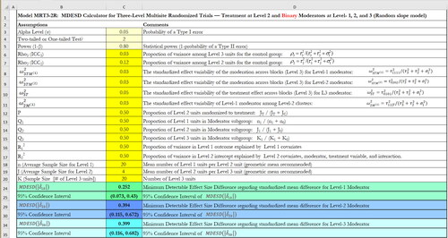
Figure 3. An example of power calculation for binary moderators at level-1, -2, and -3 with random effects in three-level MCRT.

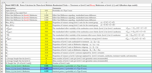
Step 2. Make reasonable assumptions about design parameter values and investigate implications across a full range of plausible values for sensitivity analysis of power

The parameters in the cells highlighted in yellow need to be input from users, for example, Cells C3-C20 in Figure 2 and Cells C3-C22 in Figure 3. Once these parameters are specified, the MDESD and their confidence intervals or power can be automatically calculated. As for all power analysis, it is critical to make reasonable assumptions about the design parameters. The type I error rate (α) is usually set as 0.05. The team chooses a two-sided test over a one-tailed test. To calculate the MDESD, the statistical power is usually set as 0.80. To calculate the statistical power to detect moderation in MCRTs, the team needs to specify the values of the design parameters: (1) the desired moderator effect size, (2) the intraclass correlation coefficients (ICCs) at cluster- and site-level (${\rho }_2={\tau }_2^2/({\tau }_3^2+{\tau }_2^2+{\sigma }_1^2)$ and ${\rho }_3={\tau }_3^2/({\tau }_3^2+{\tau }_2^2+{\sigma }_1^2),$ where ${\tau }_3^2,$ ${\tau }_2^2,$ ${\sigma }_1^2$ are the level-3, -2, and -1 variance in the unconditional model), (3) the proportions of variances explained at level-1 and -2 by covariates ($R_1^2$ and $R_2^2$), (4) the sample size at level-1, -2, and -3 (n, J, and K), and (5) the proportion of clusters assigned to the treatment group (P).

In addition, for random slope models, they need to consider the standardized effect variability of the moderation across sites for level-1 moderator (${\omega }_{{3\mathit{\text{TM}}}^{(1)}}^2={\tau }_{1111}^2/({\tau }_3^2+{\tau }_2^2+{\sigma }_1^2)$), the standardized effect variability of level-1 moderator across level-2 units (${\omega }_{{2M}^{(1)}}^2={\tau }_{11|T}^2/({\tau }_3^2+{\tau }_2^2+{\sigma }_1^2)$), the standardized effect variability of the moderation across sites for level-2 moderator (${\omega }_{{3\mathit{\text{TM}}}^{(2)}}^2={\tau }_{0202}^2/({\tau }_3^2+{\tau }_2^2+{\sigma }_1^2)$), and the standardized variability of the treatment effect across sites for level-3 moderator (${\omega }_{3T}^2={\tau }_{0101}^2/({\tau }_3^2+{\tau }_2^2+{\sigma }_1^2)$). See Dong et al. (2023a) for more detailed explanation about these parameters and Figures 2 and 3 for the example. When a moderator is a binary variable, they also need to consider the proportion of the moderator subgroup ($Q_1,$ $Q_2,$ or $Q_3$), where $Q_1,$ $Q_2,$ and $Q_3$ refer to the proportion of the individuals, clusters, and sites in one subgroup, respectively.

These design parameters can be drawn from literature or pilot studies. For example, several studies have reported the ICCs and $R_{}^2$ for academic achievement outcome measures (e.g., Hedges & Hedberg, (2007, 2013) and Kelcey et al., (2016) on mathematics and reading, and Westine et al., [2013] and Spybrook et al., (2016) on science achievement), outcome measures for teacher professional development (Kelcey & Phelps, 2013a), social and behavioral outcomes (Dong et al., 2016), and enrollment, credits earned, and degree completion for community college students (Somers et al., 2023). Table A in the appendix provides a list of key design parameters for power analysis of moderator effects in MRTs and resource examples for allocating the parameter estimates. Note that the design parameters may vary by the outcome measures and samples, and this is not an exhaustive list. Researchers may need to search and justify their design parameters based on their specific outcome measures, samples, and study designs. In particular, researchers need to consider the range of values found in the literature and the uncertainty reported for an estimated parameter value, explore the implications in terms of power and sample size and arrive at a balance among results produced from 'reasonable’ values, results produced from aberrations from those reasonable values and practical constraints (e.g., teacher sample sizes within a school are unlikely to reach 100 in most schools) so that a final selected design is efficient while also protecting against plausible deviations to the best extent available given practical constraints.

To determine the moderator effect size, researchers often draw on empirical benchmarks regarding normative expectations of annual gain, policy-relevant performance gaps, and moderation effect size results from similar studies (Bloom et al., 2008; Dong et al., 2016; Hill et al., 2008; Phelps et al., 2016). For instance, the effect sizes of disparities on concentration problems are 0.26 between black and white students, 0.43 between male and female students, and 0.33 between eligible and ineligible free/reduced price lunch students (Dong et al., 2022). The moderator effect size of a teacher classroom management program in reducing concentration problems is 0.40 favoring special education students over non-special education students (Reinke et al., 2021). These researchers may consider an effect size difference of 0.20 for their moderation study because it is equivalent to reducing 47–77% of the racial, gender, and socioeconomic disparities, and 50% of the reported moderator effect size in a similar intervention study¹.

For ICCs, Dong et al. (2016) reported that ICCs of concentration problems are 0.033 and 0.120 at school- and classroom-level, respectively. They adopted ICCs of 0.03 and 0.12 at school- and classroom-level in this demonstration. Note that these ICCs are smaller than the students’ academic outcome measures. For example, Shen et al. (2023) reported the ICCs of 0.208 and 0.067 at school-level and classroom-level for students’ math achievement. Hence, they also used ICCs of 0.20 and 0.06 at school-level and classroom-level in this demonstration.

When the pretest is included in the analysis, it can usually explain more than 50% of the variance for many educational based outcomes (Bloom et al., 2007; Dong et al., 2016; Hedges & Hedberg, 2007, 2013; Kelcey et al., 2017). As a result, it is often reasonable to assume that $R_1^2$ = $R_2^2$ = 0.5. They also adopted a balanced design, the proportion of clusters assigned to the treatment group, p = 0.5. For moderators, they assumed the proportions of the moderator subgroups, $Q_1$ = $Q_2$ = $Q_3$ =0.5.

Regarding the design parameters in the random slope models, very few empirical studies reported the values of the effect heterogeneity across sites. Weiss et al. (2017) studied 51 outcome measures in 16 two-level MIRTs and reported that the standard deviation of the treatment effect size across sites (schools) (equivalent to ${\omega }_t^{}=\sqrt{{\tau }_{11}^2/({\tau }_{00}^2+{\sigma }_{}^2)}$ in the two-level MIRTs) ranged from 0 to 0.35 with 37% ranging from [0, 0.05], 33% ranging from [0.05, 0.15], and 29% ranging from [0.15, 0.35]. Similarly, Olsen et al. (2017) studied 17 outcome measures in 6 two-level MIRTs and reported that the standard deviation of the treatment effect size across sites (schools) ranged from 0.07 to 0.31 with a mean of 0.20 and a median 0.22. Furthermore, Dong et al. (2022) reported that the standardized effect heterogeneity values for the individual-level moderators across sites (schools) (similar definition as ${\omega }_t^{},$ but with the moderator as the focal predictor) on social and behavioral outcomes range from 0.07 to 0.24 for race (White vs. Black), 0.08 to 0.24 for gender, and 0.10 to 0.24 for the free/reduced price lunch status.

Although these results cannot be directly applied to the three-level MCRT in this example because of the different designs, the researchers adopted the heterogeneity parameter values that range from moderate to large, as reported above: the standardized variability of the treatment effect across sites for level-3 moderator (${\omega }_{3T}^2$) of 0.05 and 0.10 (i.e., ${\omega }_{3T}^{}$ = 0.22 and 0.32), respectively, and the standardized effect variability of level-1 moderator across level-2 units (${\omega }_{{2M}^{(1)}}^2$) of 0.03 and 0.05, respectively (i.e., ${\omega }_{{2M}^{(1)}}^{}$ = 0.17 and 0.22). They did not identify studies reporting the standardized effect variability of the moderation across sites for level-1 moderator (${\omega }_{{3\mathit{\text{TM}}}^{(1)}}^2$) or the standardized effect variability of the moderation across sites for level-2 moderator (${\omega }_{{3\mathit{\text{TM}}}^{(2)}}^2$). They adopted ${\omega }_{{3\mathit{\text{TM}}}^{(1)}}^2$ = ${\omega }_{{3\mathit{\text{TM}}}^{(2)}}^2$ = 0.03 and 0.05, respectively. These adopted heterogeneity parameter values were at the medium to high end of the empirical distributions, leading to conservative power estimates. Furthermore, the team assumes that the sample came from typical schools, with each teacher/classroom having 20 students (n = 20) and each school having 4 teachers/classrooms (J = 4). Additionally, they explore two options for the number of schools: K = 20 and 40, respectively. Once these design parameters are input into the corresponding software module, the MDESD or power can be automatically calculated. For example, Figures 2 and 3 provide the MDESD and power calculation for binary moderators at level-1, -2, and -3 with random effects in three-level MCRTs.

Step 3. Report the results with sufficient details to replicate the analyses

The team can report the power analysis results based on the choice of study design and parameter assumptions. The research team needs to provide sufficient details for others to replicate their power analysis. The team also needs to justify the choice of their design parameter values. When there is no consensus on some design parameter values, or such values are not available, prudent practice involves conducting sensitivity analyses for power using different combinations of design parameter values that probe the plausible range of values. Table 3 provides an illustration of how research teams can summarize the MDESD and statistical power of three-level MCRTs under different assumption combinations. In addition, research teams may copy and paste some spreadsheets for power analysis as examples such as Figures 2 and 3 if there is room in their power analysis write-up. Figures S1–S6 in the supplemental materials illustrate the calculation of the MDESD and power for more examples. An example write-up of power calculation of a level-1 binary moderator effect in three-level MCRTs is provided in Appendix B.

Table 3. MDESD and statistical power of three-level MCRTs.

Level of moderator	Slope of moderator effect	${\rho }_3$=0.03, ${\rho }_2$=0.12								${\rho }_3$=0.20, ${\rho }_2$=0.06
		MDESD				Power				MDESD				Power
		Binary moderator		Continuous moderator		Binary moderator		Continuous moderator		Binary moderator		Continuous moderator		Binary moderator		Continuous moderator
		K = 20	K = 40	K = 20	K = 40	K = 20	K = 40	K = 20	K = 40	K = 20	K = 40	K = 20	K = 40	K = 20	K = 40	K = 20	K = 40
1	Nonrandomly Varying	.183	.129	.091	.065	.866	.991	1.000	1.000	.171	.121	.085	.060	.908	.996	1.000	1.000
1	Random (${\omega }_{{3\mathit{\text{TM}}}^{(1)}}^2={\omega }_{{2M}^{(1)}}^2$ = 0.03)	.252	.173	.188	.130	.606	.900	.845	.991	.242	.166	.185	.127	.640	.921	.857	.993
1	Random (${\omega }_{{3\mathit{\text{TM}}}^{(1)}}^2={\omega }_{{2M}^{(1)}}^2$ = 0.05)	.284	.195	.230	.158	.506	.818	.683	.943	.276	.190	.227	.156	.530	.841	.693	.948
2	Nonrandomly Varying	.363	.255	.182	.127	.338	.595	.869	.993	.281	.197	.140	.098	.514	.813	.979	1.000
2	Random (${\omega }_{{3\mathit{\text{TM}}}^{(2)}}^2$ = 0.03)	.394	.271	.220	.152	.297	.544	.720	.959	.313	.215	.185	.127	.434	.741	.857	.993
2	Random (${\omega }_{{3\mathit{\text{TM}}}^{(2)}}^2$ = 0.05)	.404	.278	.239	.165	.284	.522	.649	.926	.326	.224	.207	.143	.405	.704	.771	.976
3	Nonrandomly Varying	.363	.255	.182	.127	.338	.595	.870	.993	.281	.197	.140	.098	.515	.813	.979	1.000
3	Random (${\omega }_{3T}^2$ = 0.05)	.399	.300	.199	.150	.229	.425	.800	.983	.346	.260	.173	.130	.296	.545	.938	.999
3	Random (${\omega }_{3T}^2$ = 0.10)	.469	.352	.234	.176	.176	.319	.615	.906	.424	.319	.212	.159	.207	.381	.729	.963

Note. Under the assumptions: n = 20, J = 4, p = 0.5, $R_1^2$ = $R_2^2$ = 0.5, $Q_1$ = $Q_2$ = $Q_3$ = 0.5 for binary moderators, power = 0.8 for the calculation of MDESD, and effect size difference = 0.2 for the calculation of power, a two-sided test with α = 0.05.

Two-level MIRTs

The power analysis of moderation in two-level MIRTs is similar but relatively simpler than in three-level MCRTs. Consider the illustrative example introduced earlier regarding the effects of a professional development program on teacher outcomes in a two-level MIRT with teachers nested within schools (e.g., Kelcey & Phelps, 2013b). We can conduct power analysis of the moderator effects of teacher- and school-level characteristics on teacher outcomes in the two-level MIRTs. By following the same steps as in three-level MCRTs, the statistical power or MDESD can be calculated.

Step 1. Select the appropriate design and corresponding software module

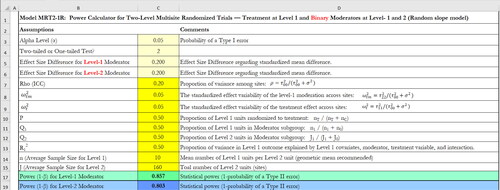
The team can choose the corresponding software modules (Columns 6–9, Table 2) to calculate the MDESD or power based on the features of their study design (e.g., random or nonrandomly varying slope, binary or continuous moderator). Suppose the team would like to conduct power analysis of moderator effect for a binary moderator (either level-1 or -2) with random slope. The team can choose Module MRT21R_MDESD for calculation of MDESD and Module MRT21R_Power for calculation of power. For instance, clicking “MRT21R_Power” will lead to the spreadsheet like Figure 4.

Figure 4. An example of power calculation for binary moderators at level-1 and -2 with random effects in two-level MIRTs.

Step 2. Make reasonable assumptions about design parameter values and investigate implications across a full range of plausible values for sensitivity analysis of power

Using a type I error rate (α) of 0.05, the team chooses a two-sided test over a one-tailed test. To calculate MDESD, the statistical power is usually set as 0.80. To calculate the statistical power to detect moderation in MCRTs, the team needs to specify the values of the design parameters: (1) the desired moderator effect size (e.g., 0.20), (2) the intraclass correlation coefficient (ICC) ($\rho ={\tau }_{00}^2/({\tau }_{00}^2+{\sigma }_{}^2),$ where ${\tau }_{00}^2$ and ${\sigma }_{}^2$ are the level-2 and −1 variance in the unconditional model), (3) the proportions of variance explained at level-1 covariates ($R_1^2$), (4) the sample size at level-1 and -2 (n and J), and (5) the proportion of individuals assigned to the treatment group (P).

Furthermore, for random slope models, the team need to consider the standardized effect variability of the moderation across sites for level-1 moderator (${\omega }_{\mathit{\text{tm}}}^2={\tau }_{22}^2/({\tau }_{00}^2+{\sigma }_{}^2),$ where ${\tau }_{22}^2$ is the variance of the random slope for the interaction term) and the standardized variability of the treatment effect across sites for level-2 moderator (${\omega }_t^2={\tau }_{11}^2/({\tau }_{00}^2+{\sigma }_{}^2),$ where ${\tau }_{11}^2$ is the variance of the random slope for the treatment variable). See Dong et al. (2021a) for more detailed explanation about these design parameters, Table 1 for the statistical models, and Figure 4 for example. When a moderator is a binary variable, the team also need to consider the proportion of the moderator subgroup ($Q_1$ or $Q_2$), where $Q_1$ and $Q_2$ refer to the proportion of the individuals and sites in one subgroup, respectively.

The design parameters should be drawn from literature or pilot studies. For example, the ICCs and $R_{}^2$ values may be found from studies listed in Table A. The researchers adopted ICC of 0.20 and $R_1^2$ = 0.5 (e.g., Kelcey & Phelps, 2013a). They also adopted a balanced design, the proportion of individuals assigned to the treatment group, p = 0.5. For moderators, they assumed the proportions of the moderator subgroups, $Q_1$ = $Q_2$ =0.5. For the standardized variability of the treatment effect across sites for level-2 moderator, they chose ${\omega }_t^2$ = 0.05 (or ${\omega }_t^{}$ = 0.22) based on Weiss et al. (2017) and Olsen et al. (2017) to get a conservative estimate of power. They did not identify studies directly reporting the standardized effect variability of the moderation across sites for level-1 moderator (${\omega }_{\mathit{\text{tm}}}^2$). However, neighboring literature suggested a value on the order of ${\omega }_{\mathit{\text{tm}}}^2$ = 0.05 (Phelps et al., 2016). Furthermore, the team assumes that the sample sizes for teachers within each school are n = 10, and for schools, J = 160. Once these design parameters are input into the corresponding software module, the MDESD or power can be automatically calculated. For example, Figure 4 provides the power calculation for binary moderators at level-1 and -2 with random effects in two-level MIRTs.

Step 3. Report the results with sufficient details to replicate the analyses

The same aforementioned principles for reporting power analysis results apply here. The team needs to provide sufficient details (e.g., the study design and parameter assumptions) for others to replicate their power analysis. The team also needs to justify the choice of their design parameters. Researchers may copy and paste the spreadsheets for power analysis in their power analysis writing, for example, reporting power calculation for binary moderator at level-1 and -2 with random slopes (Figure 4).

As noted earlier, there may not be consensus on some design parameter values, or the design parameter values are not available. Again, a sensitivity analysis using different combinations of design parameter values that consider plausible ranges of the parameter values may be useful. For example, they may choose a smaller ICC = 0.15 and larger ${\omega }_t^{}$ =${\omega }_{\mathit{\text{tm}}}^{}=$ 0.32 to get a more conservative power and MDESD estimate.

Summary of findings

To further illustrate how design parameter values affect the statistical power in three-level MCRTs, we plotted the statistical power as functions of site sample size (K) for binary moderators with four combinations of different ICCs and effect heterogeneity in Figures 5a–5d, which are analogous to the power curve for the two-level MIRTs (Figure 1 in Dong et al., 2021a). We use the same assumptions as in Table 3.

Figure 5. Power vs. site sample size for the analysis of main effects and binary moderator effects in three-level MCRTs.

Note. Under the assumptions: n = 20, J = 4, P = 0.5, $R_1^2$ = $R_2^2$ = 0.5, $Q_1$ = $Q_2$ = $Q_3$ = 0.5, effect size (standardized mean difference) for main effects = 0.2, effect size difference for binary moderator effects = 0.2, and a two-sided test with α = 0.05. ${\rho }_3$=0.03, ${\rho }_2$=0.12, ${\omega }_{{3\mathit{\text{TM}}}^{(1)}}^2={\omega }_{{2M}^{(1)}}^2$ = ${\omega }_{{3\mathit{\text{TM}}}^{(2)}}^2$ = 0.03, and ${\omega }_{3T}^2$ = 0.05 for random slope designs in Figure 5a. ${\rho }_3$=0.03, ${\rho }_2$=0.12, ${\omega }_{{3\mathit{\text{TM}}}^{(1)}}^2={\omega }_{{2M}^{(1)}}^2$ = ${\omega }_{{3\mathit{\text{TM}}}^{(2)}}^2$ = 0.05, and ${\omega }_{3T}^2$ = 0.10 for random slope designs in Figure 5b. ${\rho }_3$=0.20, ${\rho }_2$=0.06, ${\omega }_{{3\mathit{\text{TM}}}^{(1)}}^2={\omega }_{{2M}^{(1)}}^2$ = ${\omega }_{{3\mathit{\text{TM}}}^{(2)}}^2$ = 0.03, and ${\omega }_{3T}^2$ = 0.05 for random slope designs in Figure 5c. ${\rho }_3$=0.20, ${\rho }_2$=0.06, ${\omega }_{{3\mathit{\text{TM}}}^{(1)}}^2={\omega }_{{2M}^{(1)}}^2$ = ${\omega }_{{3\mathit{\text{TM}}}^{(2)}}^2$ = 0.05, and ${\omega }_{3T}^2$ = 0.10 for random slope designs in Figure 5d.

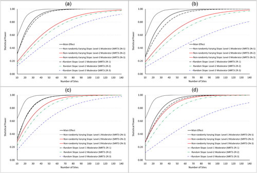
In addition, the power of main treatment effect in three-level MCRTs was calculated using PowerUp! (Dong & Maynard, 2013) and plotted for comparison. The resulting power curves are for the moderation analyses with a binary level-1 moderator with nonrandomly varying effect (black short dotted line), a binary level-2 or level-3 moderator with nonrandomly varying effect (red solid line), a binary level-1 moderator random effect (black long dotted line), a binary level-2 moderator random effect (green dotted line), a binary level-3 moderator random effect (blue dotted line), and the main treatment effect (black solid line).

We summarize the findings from Table 3 and Figure 5. First, as for all power analysis the power increases (MDESD decreases) with the sample sizes (K, J, and n). Similar as moderation in the two-level MRTs (Dong et al., 2021a), the sample sizes at different levels are not equally important. For random slope models, the high-level sample size (e.g., sites or clusters) is more important than low-level sample size (individuals). However, for nonrandomly varying slope models, the power (and MDESD) is the same for both level-2 and level-3 moderators. In these cases, the sample sizes at level-2 and level-3 are equally important and they are more important than the level-1 sample size. When considering a level-1 moderator, the importance of sample sizes at levels 1, 2, and 3 becomes equal.

Second, the proportion of the sample allocated to the treatment group (P) and to the moderator subgroup ($Q_1,$ $Q_2,$ $Q_3$) are related to the power and MDESD. The power (MDESD) increases (decreases) when P and Qs are closer to 0.5 and it achieves the maximum (minimum) value when it is a balanced design (P = $Q_1$ = $Q_2$ = $Q_3$ = 0.5).

Third, the power (MDESD) increases (decreases) when the site-level ICC increases. This is because the sites explain more level-3 variance, reduce the residual variance at level-1, and hence reduce the standard error of the moderated treatment effect estimates. The power (MDESD) increases (decreases) when the level-2 ICC increases for the analysis of a level-1 moderator, however, the power (MDESD) often decreases (increases) when the level-2 ICC increases for the analysis of level-2 and −3 moderators.

Fourth, the power increases with the proportion of level-1 variance explained by the covariates ($R_1^2$). The power also increases with the proportion of variance of level-2 intercept explained ($R_2^2$) for the analysis of level-2 and −3 moderators, however, the power for level-1 moderator analysis is not related to $R_2^2.$

Fifth, the power (MDESD) is smaller (larger) for a random slope model than a nonrandomly varying slope model for the same moderator. The differences on the power and MDESD between the two models (random slope and nonrandomly varying slope models) decreases when the effect heterogeneity decreases. In addition, the power (MDESD) is bigger (smaller) for a lower-level moderator than a higher-level moderator except for the Level-2 and −3 moderators in the nonrandomly varying slope models which have same power (MDESD).

Sixth, the MDESD as defined by the standardized mean difference for the binary moderator when $Q_1$ = $Q_2$ = $Q_3$ = 0.5 is always twice the value of the MDESD defined by the standardized coefficient for the continuous moderator with a nonrandomly varying effect.

Finally, the power of a nonrandomly varying slope model for level-1 moderator is always larger than the main effect analysis. The power of a random slope model for level-1 moderator is close to the main effect analysis.

Conclusion

In this tutorial, we demonstrated and discussed power analyses for moderator effects in three-level MCRTs and two-level MIRTs using the software. To effectively utilize this tool, it is crucial to follow three steps: (1) select the suitable design and corresponding software modules, (2) make reasonable assumptions about design parameters and explore the implications across the full range of parameter values, and (3) present the results with sufficient details.

It is important to note that there is inherent uncertainty (variance) in the parameter estimates found in the literature, the target population might differ from the population for which the design parameters were estimated in previous studies, and the design parameter estimates might not be always available. In such cases, researchers can sometimes rely on design parameter results from pilot studies or results from comparable outcomes and designs. However, we recommend conducting sensitivity analyses of the power by carefully considering estimates under a plausible range of design parameter values. This underscores the need for more research on design parameters, particularly focusing on the heterogeneous effects of the moderator variable, treatment, and moderation.

Disclosure statement

No potential conflict of interest was reported by the author(s).

Additional information

Funding

This project has been funded by the National Science Foundation [1913563; 1760884] and the Institute of Education Sciences [R305D190013]. The opinions expressed herein are those of the authors and not the funding agencies.

Notes

1 These percentages are calculated by dividing the target moderator effect size (0.20) by the disparity or reported moderator effect size in a similar intervention, for example, 0.20/0.26 = 77%, 0.20/0.43 = 47%, 0.20/0.33 = 61%, and 0.20/0.40 = 50%.

Appendix A: Table A

Design parameter resources.

3-level MCRTs

Table

Parameter	Comments	Resources
${\rho }_3$	Intraclass correlation coefficient at level 3: Proportion of variance among Level 3 units: ${\rho }_3={\tau }_3^2/({\tau }_3^2+{\tau }_2^2+{\sigma }_1^2).$	Social & Behavior: Dong et al. (2016); Jacob et al. (2010) Math: Wijekumar et al. (2009); Westine et al. (2013); McCoach et al. (2014); Shen et al. (2023); Zhu et al. (2012); Hedges and Hedberg (2013) Reading: Drummond et al. (2011); Wijekumar et al. (2014); Westine et al. (2013); Shen et al. (2023); Zhu et al. (2012) Science: Westine et al. (2013); Spybrook et al. (2016); Zhu et al. (2012)
${\rho }_2$	Intraclass correlation coefficient at level 2: Proportion of variance among Level 2 units: ${\rho }_2={\tau }_2^2/({\tau }_3^2+{\tau }_2^2+{\sigma }_1^2).$	Social & Behavior: Dong et al. (2016); Jacob et al. (2010) Math: Wijekumar et al. (2009); Westine et al. (2013); McCoach et al. (2014); Shen et al. (2023); Zhu et al. (2012); Hedges and Hedberg (2013) Reading: Drummond et al. (2011); Wijekumar et al. (2014); Westine et al. (2013); Shen et al. (2023); Zhu et al. (2012) Science: Westine et al. (2013); Spybrook et al. (2016); Zhu et al. (2012)
$R_2^2$	Proportion of variance in Level 2 intercept explained by Level 2 covariates	Social & Behavior: Dong et al. (2016); Jacob et al. (2010) Math: Wijekumar et al. (2009); Westine et al. (2013); McCoach et al. (2014); Shen et al. (2023); Zhu et al. (2012); Hedges and Hedberg (2013) Reading: Drummond et al. (2011); Wijekumar et al. (2014); Westine et al. (2013); Shen et al. (2023); Zhu et al. (2012) Science: Westine et al. (2013); Spybrook et al. (2016); Zhu et al. (2012)
$R_1^2$	Proportion of variance in Level 1 outcome explained by Level 1 covariates	Social & Behavior: Dong et al. (2016); Jacob et al. (2010) Math: Wijekumar et al. (2009); Westine et al. (2013); McCoach et al. (2014); Shen et al. (2023); Zhu et al. (2012); Hedges and Hedberg (2013) Reading: Drummond et al. (2011); Wijekumar et al. (2014); Westine et al. (2013); Shen et al. (2023); Zhu et al. (2012) Science: Westine et al. (2013); Spybrook et al. (2016); Zhu et al. (2012)
${\omega }_{3T}^2$	The standardized effect variability of the treatment effect across blocks (Level 3) for L3 moderator:${\omega }_{3T}^2={\tau }_{0101}^2/({\tau }_3^2+{\tau }_2^2+{\sigma }_1^2).$	Math: Wijekumar et al. (2009) Reading: Drummond et al. (2011); Wijekumar et al. (2014)

2-level MRTs

Table

Parameter	Comments	Resources
${\rho }_{}$	Intraclass correlation coefficient: Proportion of variance among Level 2 units: ${\rho }_{}={\tau }_{00}^2/({\tau }_{00}^2+{\sigma }_{}^2).$	Social & Behavior: Dong et al. (2016) Math: Westine et al. (2013); Hedges and Hedberg (2007); Bloom et al. (2007); Zhu et al. (2012) Reading: Drummond et al. (2011); Westine et al. (2013); Hedges and Hedberg (2007); Bloom et al. (2007); Zhu et al. (2012) Science: Spybrook et al. (2016); Zhu et al. (2012) Teacher outcomes: Kelcey and Phelps (2013a); Kelcey and Phelps (2013b)
$R_1^2$	Proportion of variance in Level 1 outcome explained by Level 1 covariates	Social & Behavior: Dong et al. (2016) Math: Westine et al. (2013); Hedges and Hedberg (2007); Bloom et al. (2007); Zhu et al. (2012) Reading: Drummond et al. (2011); Westine et al. (2013); Hedges and Hedberg (2007); Bloom et al. (2007); Zhu et al. (2012) Science: Spybrook et al. (2016); Zhu et al. (2012) Teacher outcomes: Kelcey and Phelps (2013a); Kelcey and Phelps (2013b)

Appendix B:

 An example of write-up of power calculation of a level-1 binary moderator effect in three-level MCRTs

In this three-level MCRT designed to investigate a binary level-1 moderator effect in reducing concentration problems among 5^th graders, we made the following assumptions: (1) Our desired moderation effect size is 0.20, equivalent to reducing 47-77% of the racial, gender, and socioeconomic disparities (Dong et al., 2022), and 50% of the reported moderator effect size in a similar intervention study (Reinke et al., 2021). (2) The intra-class correlations at the school- and classroom-level are 0.03 and 0.12, respectively (Dong et al., 2016) and 0.20 and 0.06, respectively (Shen et al., 2023). (3) The proportions of variance explained by the pretest at level 1 is 50% (Dong et al., 2016). (4) It is a balanced design, with the proportion of classrooms assigned to the treatment group being p = 0.5, and the proportion of the moderator subgroup being Q₁ = 0.5. (5). To be conservative, we use a random slope model. We did not identify any studies reporting the heterogeneity parameter values for the treatment or moderator variable in three-level MCRT. Hence, we adopted the heterogeneity parameter values at the medium to high end of the empirical distributions reported in the literature for two-level MIRTs (Dong et al., 2022; Olsen et al., 2017; Weiss et al., 2017) as approximation. The standardized effect variability of level-1 moderator across level-2 units (${\omega }_{{2M}^{(1)}}^2$) are 0.03 and 0.05, respectively. The standardized effect variability of the moderation across sites for level-1 moderator (${\omega }_{{3\mathit{\text{TM}}}^{(1)}}^2$) are 0.03 and 0.05, respectively. (6) The sample came from typical schools, with each classroom having 20 students (n = 20) and each school having 4 classrooms (J = 4) at grade 5. Additionally, we explore two options for the number of schools: K = 20 and 40, respectively. (7) The type I error rate (α) is set as 0.05, and we choose a two-sided test. According to the spreadsheet in PowerUp!-Moderator-MRTs (Dong et al., 2023a), the statistical power from the combinations of parameters assumed above ranges from 0.51 to 0.64 for K = 20 and from 0.82 to 0.92 for K = 40.

References

- Barr, D. J., Levy, R., Scheepers, C., & Tily, H. J. (2013). Random effects structure for confirmatory hypothesis testing: Keep it maximal. Journal of Memory and Language, 68(3), 255–278. https://doi.org/10.1016/j.jml.2012.11.001
- Bates, D., Kliegl, R., Vasishth, S., & Baayen, H. (2015). Parsimonious mixed models. arXiv preprint arXiv:1506.04967.
- Bloom, H. S., & Spybrook, J. (2017). Assessing the precision of multisite trials for estimating the parameters of a cross-site population distribution of program effects. Journal of Research on Educational Effectiveness, 10(4), 877–902. https://doi.org/10.1080/19345747.2016.1271069
- Bloom, H. S., Hill, C. J., Black, A. B., & Lipsey, M. W. (2008). Performance trajectories and performance gaps as achievement effect-size benchmarks for educational interventions. Journal of Research on Educational Effectiveness, 1(4), 289–328. https://doi.org/10.1080/19345740802400072
- Bloom, H. S., Richburg-Hayes, L., & Black, A. R. (2007). Using covariates to improve precision for studies that randomize schools to evaluate educational interventions. Educational Evaluation and Policy Analysis, 29(1), 30–59. https://doi.org/10.3102/0162373707299550
- Dong, N., Herman, K. C., Reinke, W. M., Wilson, S. J., & Bradshaw, C. P. (2022). Gender, racial, and socioeconomic disparities on social and behavioral skills for K-8 students with and without interventions: An integrative data analysis of eight cluster randomized trials. Prevention Science, 24(8), 1483–1498. Advance online publication. https://doi.org/10.1007/s11121-022-01425-w
- Dong, N., Kelcey, B., & Spybrook, J. (2018). Power analyses of moderator effects in three-level cluster randomized trials. The Journal of Experimental Education, 86(3), 489–514. https://doi.org/10.1080/00220973.2017.1315714
- Dong, N., Kelcey, B., & Spybrook, J. (2021a). Design considerations in multisite randomized trials to probe moderated treatment effects. Journal of Educational and Behavioral Statistics, 46(5), 527–559. https://doi.org/10.3102/1076998620961492
- Dong, N., Kelcey, B., & Spybrook, J. (2023a). Experimental design and power for moderation in multisite cluster randomized trials. The Journal of Experimental Education, 1–17. https://doi.org/10.1080/00220973.2023.2226934
- Dong, N., Kelcey, B., & Spybrook, J. (2023b). Identifying and estimating causal moderation for treated and targeted subgroups. Multivariate Behavioral Research, 58(2), 221–240. https://doi.org/10.1080/00273171.2022.2046997
- Dong, N., Kelcey, B., Spybrook, J., Maynard, R. A. (2023c). PowerUp!-Moderator-MRTs: A tool for calculating statistical power and minimum detectable effect size differences of the moderator effects in multisite randomized trials. http://www.causalevaluation.org/.
- Dong, N., & Maynard, R. A. (2013). PowerUp!: A tool for calculating minimum detectable effect sizes and minimum required sample sizes for experimental and quasi-experimental design studies. Journal of Research on Educational Effectiveness, 6(1), 24–67. https://doi.org/10.1080/19345747.2012.673143
- Dong, N., Reinke, W. M., Herman, K. C., Bradshaw, C. P., & Murray, D. W. (2016). Meaningful effect sizes, intraclass correlations, and proportions of variance explained by covariates for panning two- and three-level cluster randomized trials of social and behavioral outcomes. Evaluation Review, 40(4), 334–377. https://doi.org/10.1177/0193841X16671283
- Dong, N., Spybrook, J., Kelcey, B., & Bulus, M. (2021b). Power analyses for moderator effects with (non)random slopes in cluster randomized trials. Methodology, 17(2), 92–110. https://doi.org/10.5964/meth.4003
- Drummond, K., Chinen, M., Duncan, T. G., Miller, H., Fryer, L., Zmach, C., & Culp, K. (2011). Impact of the thinking reader [r] software program on grade 6 reading vocabulary, comprehension, strategies, and motivation: Final report. NCEE 2010-4035. National Center for Education Evaluation and Regional Assistance.
- Hedges, L. V., & Hedberg, E. (2007). Intraclass correlation values for planning group randomized trials in education. Educational Evaluation and Policy Analysis, 29(1), 60–87. https://doi.org/10.3102/0162373707299706
- Hedges, L. V., & Hedberg, E. (2013). Intraclass correlations and covariate outcome correlations for planning two- and three-level cluster-randomized experiments in education. Evaluation Review, 37(6), 445–489. https://doi.org/10.1177/0193841X14529126
- Hill, C. J., Bloom, H. S., Black, A. R., & Lipsey, M. W. (2008). Empirical benchmarks for interpreting effect sizes in research. Child Development Perspectives, 2(3), 172–177. https://doi.org/10.1111/j.1750-8606.2008.00061.x
- Jacob, R., Zhu, P., & Bloom, H. (2010). New empirical evidence for the design of group randomized trials in education. Journal of Research on Educational Effectiveness, 3(2), 157–198. https://doi.org/10.1080/19345741003592428
- Kelcey, B., & Phelps, G. (2013a). Considerations for designing group randomized trials of professional development with teacher knowledge outcomes. Educational Evaluation and Policy Analysis, 35(3), 370–390. https://doi.org/10.3102/0162373713482766
- Kelcey, B., & Phelps, G. (2013b). Strategies for improving power in school-randomized studies of professional development. Evaluation Review, 37(6), 520–554. https://doi.org/10.1177/0193841X14528906
- Kelcey, B., Hill, H., & Chin, M. (2019). Teacher mathematical knowledge, instructional quality, and student outcomes: A multilevel mediation quantile analysis. School Effectiveness and School Improvement, 30(4), 398–431. https://doi.org/10.1080/09243453.2019.1570944
- Kelcey, B., Phelps, G., Spybrook, J., Jones, N., & Zhang, J. (2017). Designing large-scale multisite and cluster-randomized studies of professional development. The Journal of Experimental Education, 85(3), 389–410. https://doi.org/10.1080/00220973.2016.1220911
- Kelcey, B., Shen, Z., & Spybrook, J. (2016). Intraclass correlation coefficients for designing school randomized trials in education in Sub-Saharan Africa. Evaluation Review, 40(6), 500–525. https://doi.org/10.1177/0193841X16660246
- Kelcey, B., Spybrook, J., & Dong, N. (2019). Sample size planning in cluster-randomized studies of multilevel mediation. Prevention Science: The Official Journal of the Society for Prevention Research, 20(3), 407–418. https://doi.org/10.1007/s11121-018-0921-6
- Kelcey, B., Spybrook, J., Dong, N., & Bai, F. (2020). Cross-level mediation in school-randomized studies of teacher development: Experimental design and power. Journal of Research on Educational Effectiveness, 13(3), 459–487. https://doi.org/10.1080/19345747.2020.1726540
- Matuschek, H., Kliegl, R., Vasishth, S., Baayen, H., & Bates, D. (2017). Balancing Type I error and power in linear mixed models. Journal of Memory and Language, 94, 305–315. https://doi.org/10.1016/j.jml.2017.01.001
- McCoach, D. B., Gubbins, E. J., Foreman, J., Rubenstein, L. D., & Rambo-Hernandez, K. E. (2014). Evaluating the efficacy of using predifferentiated and enriched mathematics curricula for grade 3 students: A multisite cluster-randomized trial. Gifted Child Quarterly, 58(4), 272–286. https://doi.org/10.1177/0016986214547631
- Olsen, R., Bein, E., & Judkins, D. (2017). Sample size requirements for education multi-site RCTs that select sites randomly. SSRN Electronic Journal. https://doi.org/10.2139/ssrn.2956576
- Phelps, G., Kelcey, B., Liu, S., & Jones, N. (2016). Informing estimates of program effects for studies of mathematics professional development using teacher content knowledge outcomes. Evaluation Review, 40(5), 383–409. https://doi.org/10.1177/0193841X16665024
- Raudenbush, S. W., & Bryk, A. S. (2002). Hierarchical linear models: Applications and data analysis methods. (2nd ed.). Sage.
- Raudenbush, S. W., & Liu, X. (2000). Statistical power and optimal design for multisite randomized trials. Psychological Methods, 5(2), 199–213. https://doi.org/10.1037/1082-989x.5.2.199
- Reinke, W. M., Stormont, M., Herman, K. C., & Dong, N. (2021). The incredible years teacher classroom management program: Effects for students receiving special education services. Remedial and Special Education, 42(1), 7–17. https://doi.org/10.1177/0741932520937442
- Seedorff, M., Oleson, J., & McMurray, B. (2019). Maybe maximal: Good enough mixed models optimize power while controlling Type I error. https://doi.org/10.31234/osf.io/xmhfr
- Shen, Z., Curran, F. C., You, Y., Splett, J. W., & Zhang, H. (2023). Intraclass correlations for evaluating the effects of teacher empowerment programs on student educational outcomes. Educational Evaluation and Policy Analysis, 45(1), 134–156. https://doi.org/10.3102/01623737221111400
- Somers, M.-A., Weiss, M. J., & Hill, C. (2023). Design parameters for planning the sample size of individual-level randomized controlled trials in community colleges. Evaluation Review, 47(4), 599–629. https://doi.org/10.1177/0193841X221121236
- Spybrook, J., & Raudenbush, S. W. (2009). An Examination of the precision and technical accuracy of the first wave of group-randomized trials funded by the institute of education sciences. Educational Evaluation and Policy Analysis, 31(3), 298–318. https://doi.org/10.3102/0162373709339524
- Spybrook, J., Shi, R., & Kelcey, B. (2016). Progress in the past decade: An examination of the precision of cluster randomized trials funded by the U.S. institute of education sciences. International Journal of Research & Method in Education, 39(3), 255–267. https://doi.org/10.1080/1743727X.2016.1150454
- Spybrook, J., Westine, C. D., & Taylor, J. A. (2016). Design parameters for impact research in science education: A multistate analysis. AERA Open, 2(1), 233285841562597. https://doi.org/10.1177/2332858415625975
- U.S. Department of Education Institute of Education Sciences & National Science Foundation (2013). August). Common Guidelines for Education Research and Development (NSF 13–126). http://ies.ed.gov/pdf/CommonGuidelines.pdf
- Weiss, M. J., Bloom, H. S., Verbitsky-Savitz, N., Gupta, H., Vigil, A. E., & Cullinan, D. N. (2017). How much do the effects of education and training programs vary across sites? Evidence from past multisite randomized trials. Journal of Research on Educational Effectiveness, 10(4), 843–876. https://doi.org/10.1080/19345747.2017.1300719
- Weiss, M., Bloom, H. S., & Brock, T. (2014). A conceptual framework for studying the sources of variation in program effects. Journal of Policy Analysis and Management, 33(3), 778–808. https://doi.org/10.1002/pam.21760
- Westine, C. D., Spybrook, J., & Taylor, J. A. (2013). An empirical investigation of variance design parameters for planning cluster-randomized trials of science achievement. Evaluation Review, 37(6), 490–519. https://doi.org/10.1177/0193841X14531584
- Wijekumar, K., Hitchcock, J., Turner, H., Lei, P., & Peck, K. (2009). A multisite cluster randomized trial of the effects of compass learning Odyssey [R] math on the math achievement of selected grade 4 students in the Mid-Atlantic Region. Final Report. NCEE 2009-4068. National Center for Education Evaluation and Regional Assistance.
- Wijekumar, K., Meyer, B. J., Lei, P. W., Lin, Y. C., Johnson, L. A., Spielvogel, J. A., Shurmatz, K. M., Ray, M., & Cook, M. (2014). Multisite randomized controlled trial examining intelligent tutoring of structure strategy for fifth-grade readers. Journal of Research on Educational Effectiveness, 7(4), 331–357. https://doi.org/10.1080/19345747.2013.853333
- Zhu, P., Jacob, R., Bloom, H., & Xu, Z. (2012). Designing and analyzing studies that randomize schools to estimate intervention effects on student academic outcomes without classroom-level information. Educational Evaluation and Policy Analysis, 34(1), 45–68. https://doi.org/10.3102/0162373711423786