Minimum Regularized Covariance Trace Estimator and Outlier Detection for Functional Data

Abstract

We propose the Minimum Regularized Covariance Trace (MRCT) estimator, a novel method for robust covariance estimation and functional outlier detection designed primarily for dense functional data. The MRCT estimator employs a subset-based approach that prioritizes subsets exhibiting greater centrality based on the generalization of the Mahalanobis distance, resulting in a fast-MCD type algorithm. Notably, the MRCT estimator handles high-dimensional datasets without the need for preprocessing or dimension reduction techniques, due to the internal smoothening whose amount is determined by the regularization parameter $\alpha >0$. The selection of α is automated. An extensive simulation study demonstrates the efficacy of the MRCT estimator in terms of robust covariance estimation and automated outlier detection, emphasizing the balance between noise exclusion and signal preservation achieved through appropriate selection of α. The method converges fast in practice and performs favorably when compared to other functional outlier detection methods.

Keywords:

• Functional outlier detection
• Mahalanobis distance
• Robust covariance estimator
• Regularization

1 Introduction

The analysis of functional data is becoming increasingly important in many fields, including medicine, biology, finance, and engineering, among others. Functional data are characterized by measurements that are taken over a continuum, such as time or space, and are often modeled as curves or surfaces. One important aspect of functional data analysis is the estimation of the covariance structure, as it holds significance across different tasks like smoothing, regression, and classification. However, the estimation of the covariance structure for functional data is challenging, especially in the presence of outliers or other sources of noise. Traditional covariance estimators, such as for example the sample covariance, are sensitive to outliers and may produce unreliable results. Therefore, the development of robust covariance estimators that can handle outliers and other types of noise is an active area of research in functional data analysis.

Several robust covariance estimators have been proposed for functional data in the literature. These estimators are based on different approaches, such as trimming, shrinkage, or rank-based methods, and they aim to produce estimates that are less sensitive to outliers and can further be combined with outlier detection techniques to identify functional outliers and improve the overall quality of the analysis; see for example Boente and Salibián-Barrera (2021), Locantore et al. (1999), Cuevas, Febrero, and Fraiman (2007), Gervini (2008), and Sawant, Billor, and Shin (2012). In this article, we propose a novel robust covariance estimator based on a trimmed-sample covariance, designed primarily for dense functional data. The approach is motivated by the multivariate trimmed covariance estimator chosen such that it minimizes the Kullback-Leibler divergence between the underlying data distribution and the estimated distribution. The article is structured as follows: Section 2 introduces notation and important properties of the covariance operator in the Hilbert space of square-integrable functions on an interval. Section 3 motivates and introduces the proposed MRCT estimator, followed by a discussion on its algorithmic aspects in Section 4. We evaluate the performance of the estimator through the simulation study detailed in Section 5 for Gaussian random processes, and in supplement Section E for t-distributed processes (see e.g., Bånkestad et al. 2020), and white noise. A real-data analysis is given in Section 6. The proofs of technical results are available in supplement Section C.

2 Notation

Let X be a random function on $L^2(I)$, that is the Hilbert space of square-integrable functions over the interval I. Denote $\mu (t)=\mathbb{E}(X(t)),t\in I$ to be the mean of X, where for the simplicity of the notation, we assume that μ = 0. Let further $C:L^2(I)\to L^2(I)$ be the corresponding covariance operator defined by $\mathit{\text{Cx}}(t)=\mathbb{E}(〈x,X-\mu 〉(X(t)-\mu (t)))$, for $x\in L^2(I)$, $t\in I$. In continuation, we will drop the argument t, as the summation and multiplication of functions are naturally defined element-wise.

We denote ${\psi }_i:I\to \mathbb{R}$ and ${\lambda }_i\ge 0,i\ge 1$ to be the ith eigenfunction and eigenvalue of C, respectively, that is, $C{\psi }_i={\lambda }_i{\psi }_i$ for $i=1,2,\dots$. Thus, C admits the spectral decomposition $\mathit{\text{Cx}}={\sum }_{i=1}^{\infty }{\lambda }_i〈{\psi }_i,x〉{\psi }_i\hspace{1em}\forall x\in L^2(I),$ where the convergence of the partial sums is in the operator norm. It can be shown that C is a trace-class operator, implying that $\sum _i{\lambda }_i<\infty$ (Ramsay and Silverman 1997). Let further $X_1,\dots ,X_n$ be a functional random sample from $L^2(I)$. For the subset $H\subset \{1,2,\dots ,n\},\left|H\right|=h$, $n/2\le h\le n$ we define $$\begin{array}{c}{\overline{X}}_H=\frac{1}{h}\sum _{i\in H}{X}_i,\\ {\widehat{C}}_H(X)=\frac{1}{h}\sum _{i\in H}(X_i-\overline{X})\otimes (X_i-{\overline{X}}_H),\hspace{1em}\text{and}\\ {\widehat{C}}_H{(X)}^{\text{NC}}=\frac{1}{h}\sum _{i\in H}{X}_i\otimes X_i,\end{array}$$to be the trimmed sample mean, covariance, and non-centered covariance operators, respectively, calculated at the subset H. We denote further ${\widehat{\psi }}_{i,H}$ to be the i-th eigenfunction of ${\widehat{C}}_H$, with the corresponding eigenvalue ${\widehat{\lambda }}_{i,H}$, that is, ${\widehat{C}}_H{\widehat{\psi }}_{i,H}={\widehat{\lambda }}_{i,H}{\widehat{\psi }}_{i,H}$, $i=1,2,\dots$. It can then also be shown that ${\widehat{C}}_H$ is a trace-class operator admitting an eigendecomposition ${\widehat{C}}_{H}x={\sum }_{i=1}^{\infty }{\widehat{\lambda }}_{i,H}〈{\widehat{\psi }}_{i,H},x〉{\widehat{\psi }}_{i,H}$. For more details on important properties of the covariance operator in the Hilbert space $L^2(I)$ see Section A in the supplement.

3 Minimum Regularized Covariance Trace Estimator

3.1 Motivation

In the multivariate setting, given the random sample ${\mathbf{x}}_1,\dots ,{\mathbf{x}}_n\in {\mathbb{R}}^p$ from a distribution with mean $\mathit{\mu }$ and covariance $\mathbf{\Sigma }$, one approach to robustify the estimation of the mean and the covariance is to use the weighted sample estimators, which assign different weights, $w_1,\dots ,w_n\ge 0$, to different data points based on their relative importance. In this approach, outlying or noisy data points ought to be given smaller weights, thus, reducing their impact on the estimated mean and covariance. Especially, choosing weights $w_i\in \{0,1\},i=1,\dots ,n$, with the constraint ${\sum }_{i=1}^n{w}_i=h$, for some fixed $n/2\le h\le n$, yields trimmed mean and covariance estimators. One of the most widely used members of this class of estimators is the so-called Minimum Covariance Determinant (MCD) estimator (Rousseeuw and Driessen 1999). For a given fixed number h, which is roughly half of the sample size n, its objective is to select h (out of n) observations for which the calculated sample covariance matrix has the lowest determinant. In the parametric family of distributions parameterized by its mean and covariance, we employ a similar strategy, however, with the objective to minimize the Kullback-Leibler (KL) divergence between the theoretical (underlying data distribution) and the one parameterized by the estimates of mean and the covariance, using corresponding sample estimates calculated at a subset $H\subset \{1,\dots ,n\},\left|H\right|=h$. The KL divergence between continuous distributions P and Q with densities f_P and f_Q, respectively, denoted as $\text{KL}(P\parallel Q):={\mathbb{E}}_Q(\hspace{0.17em}\mathrm{\text{log}}\hspace{0.17em}(f_P(\mathbf{x})/\hspace{0.17em}\mathrm{\text{log}}\hspace{0.17em}(f_Q(\mathbf{x})))$, is a measure of how far the probability distribution P is from a second, reference probability distribution Q Kullback and Leibler (1951) and Kullback (1959). Assume now the data ${\mathbf{x}}_1,\dots ,{\mathbf{x}}_n$ originate from a normal distribution $\mathcal{N}(\mathbf{0},\mathbf{\Sigma })$, and denote ${\overline{\mathbf{x}}}_H$ and ${\widehat{\mathbf{\Sigma }}}_H(\mathbf{x})$ to be the mean and the covariance of $\{{\mathbf{x}}_i;i\in H\}$. Denote further ${\widehat{\mathbf{\Sigma }}}_H^{\text{NC}}(\mathbf{x})=\frac{1}{h}\sum _{i\in H}{\mathbf{x}}_i{\mathbf{x}}_i^{\prime }$ to be the “non-centered” covariance of an h-subset H. The KL divergence between $\mathcal{N}(\mathbf{0},\mathbf{\Sigma })$ and $\mathcal{N}({\overline{\mathbf{x}}}_H,{\widehat{\mathbf{\Sigma }}}_H(\mathbf{x}))$ is (1) $$\begin{array}{c}\text{KL}(\mathcal{N}(\mathbf{0},\mathbf{\Sigma })||\mathcal{N}({\overline{\mathbf{x}}}_H,{\widehat{\mathbf{\Sigma }}}_H(\mathbf{x})))\\ \mathrm{\hspace{1em}}\mathrm{\hspace{1em}}=\text{tr}({\mathbf{\Sigma }}^{-1}{\widehat{\mathbf{\Sigma }}}_H^{\text{NC}}(\mathbf{x}))+\hspace{0.17em}\mathrm{\text{log}}\hspace{0.17em}(\mathrm{\text{det}}({\mathbf{\Sigma }}^{-1}{\widehat{\mathbf{\Sigma }}}_H(\mathbf{x})))-p;\end{array}$$(1) see Zhang et al. (2023) for more details. As the calculation of (1) in practice involves the estimation of the density function, direct use of KL divergence is usually mitigated by the use of appropriate approximations; see for example Blei, Kucukelbir, and McAuliffe (2017) for more details. Observe, therefore, that $\hspace{0.17em}\mathrm{\text{log}}\hspace{0.17em}(\mathrm{\text{det}}({\mathbf{\Sigma }}^{-1/2}{\widehat{\mathbf{\Sigma }}}_H(\mathbf{x}){\mathbf{\Sigma }}^{-1/2}))=\hspace{0.17em}\mathrm{\text{log}}\hspace{0.17em}(\mathrm{\text{det}}({\widehat{\mathbf{\Sigma }}}_H(\mathbf{y})))$, where ${\widehat{\mathbf{\Sigma }}}_H(\mathbf{y})$ represents the covariance of standardized observations ${\mathbf{y}}_i={\mathbf{\Sigma }}^{-1/2}{\mathbf{x}}_i:i\in H$. For ${\mathbf{y}}_i$ we have that $\text{cov}(\mathbf{y})={\mathbf{I}}_p$, indicating that any strongly consistent estimator of $\text{cov}(\mathbf{y})$ admits the representation ${\mathbf{I}}_p+{\epsilon }_n{\mathbf{M}}_n$, where ${\mathbf{M}}_n$ is a unit-norm p × p matrix and ${\epsilon }_n{\to }_{a.s.}0$. This holds in particular for the consistent estimator ${\widehat{\mathbf{\Sigma }}}_H^{\text{NC}}(\mathbf{y})={\mathbf{I}}_p+{\epsilon }_n{\mathbf{M}}_n$, for some unit-norm p × p matrix ${\mathbf{M}}_n$. A slight modification of Jacobi’s formula implies that the directional derivative of the determinant in the direction of ${\mathbf{M}}_n$ evaluated at the identity equals the trace of ${\mathbf{M}}_n$, that is $\underset{{\epsilon }_n\to 0}{\mathrm{\text{lim}}}(\mathrm{\text{det}}({\mathbf{I}}_p+{\epsilon }_n{\mathbf{M}}_n)‐\mathrm{\text{det}}({\mathbf{I}}_p))/{\epsilon }_n=\text{tr}({\mathbf{M}}_n)$. Matrix determinant lemma (Lemma 1 in Ding and Zhou (2007)) gives that $\mathrm{\text{det}}({\widehat{\mathbf{\Sigma }}}_H(\mathbf{y}))=\mathrm{\text{det}}({\widehat{\mathbf{\Sigma }}}_H^{\text{NC}}(\mathbf{y}))+{\overline{\mathbf{x}}}_H^{\prime }\text{adj}({\widehat{\mathbf{\Sigma }}}_H^{\text{NC}}(\mathbf{y})){\overline{\mathbf{x}}}_H$, where for a regular square matrix A, $\text{adj}(\mathbf{A})$ denotes adjugate of A. Furthermore, the normality of the sample y along with the consistency of the sample covariance estimator ${\widehat{\mathbf{\Sigma }}}_H^{\text{NC}}$ ensure that we can bound ${\overline{\mathbf{x}}}_H^{\prime }\text{adj}({\widehat{\mathbf{\Sigma }}}_H^{\text{NC}}(\mathbf{y})){\overline{\mathbf{x}}}_H=O({\delta }_n^2)$, where $\Vert {\overline{\mathbf{x}}}_H\Vert \le {\delta }_n$, for ${\delta }_n{\to }_{a.s.}0$. Applying further the first order Taylor expansion of $\mathrm{\text{det}}({\widehat{\mathbf{\Sigma }}}_H^{\text{NC}}(\mathbf{y}))$ around the identity yields that $$\begin{array}{c}\text{det}({\widehat{\mathbf{\Sigma }}}_H(\mathbf{y}))=\text{det}({\widehat{\mathbf{\Sigma }}}_H^{\text{NC}}(\mathbf{y}))+o({\delta }_n^2)\\ =\mathrm{\text{det}}({\mathbf{I}}_p)+{\epsilon }_n\text{tr}({\mathbf{M}}_n)+O({\epsilon }_n^2)+O({\delta }_n^2)\\ =\text{tr}({\mathbf{\Sigma }}^{-1}{\widehat{\mathbf{\Sigma }}}_H^{\text{NC}}(\mathbf{x}))-(p-1)+O({\epsilon }_n^2)+O({\delta }_n^2).\end{array}$$

This result implies that for sufficiently large n, the determinant of the consistent estimator of the covariance of the standardized observations is arbitrarily well approximated by its trace. Thus, instead of directly minimizing $\text{KL}(\mathcal{N}(\mathbf{0},\mathbf{\Sigma }),\mathcal{N}({\overline{\mathbf{x}}}_H,{\widehat{\mathbf{\Sigma }}}_H(\mathbf{x})))$ over all subsets $\left|H\right|=h$, we consider the following optimization problem (2) $$H_0=\text{arg} {\mathrm{\text{min}}}_{H\subset \{1,\dots ,n\}:\left|H\right|=h}\text{tr}\left({\widehat{\mathbf{\Sigma }}}_H^{\text{NC}}(\mathbf{y})\right)=\text{arg} {\mathrm{\text{min}}}_{H\subset \{1,\dots ,n\}:\left|H\right|=h}\sum _{i\in H}\Vert {\mathbf{y}}_i{\Vert }^2,$$(2) where ${\widehat{\mathbf{\Sigma }}}_H^{\text{NC}}(\mathbf{y})=\frac{1}{h}\sum _{i\in H}{\mathbf{y}}_i{\mathbf{y}}_i^{\prime }$ is a non-centered covariance of standardized observations $\{{\mathbf{y}}_i={\mathbf{\Sigma }}^{-1/2}{\mathbf{x}}_i:i\in H\}$. The corresponding estimators ${\widehat{\mathbf{\Sigma }}}_{H_0}(\mathbf{x})$ and ${\overline{\mathbf{x}}}_{H_0}$ of the covariance and the mean are referred to as multivariate Minimum Covariance Trace (MCT) estimator of the mean and the covariance, respectively. It should be noted that the strategy of minimization of an approximation does not necessarily yield a solution close to the target one. Specifically, even though the KL divergence (1) and the appropriate monotonically increasing transformation of an approximated trace loss (2) are arbitrarily close to each other, optimal subsets based on these two losses could be different. However, Section B.1 in the supplement provides reassurance that the likelihood of such an event is negligible.

The optimization problem (2) highlights the need for an appropriate standardization of the data when extending this approach to more general spaces, with the standardization ensuring that the norm of the standardized object reflects a specific dissimilarity measure of the object from its corresponding mean. In the multivariate setting, the norm of the standardized observations ${\mathbf{y}}_i$ corresponds to the Mahalanobis distance of ${\mathbf{x}}_i$, while in the functional setting, an appropriate standardization will result in a random function whose norm equals the α-Mahalanobis distance (3.1) introduced in Berrendero, Bueno-Larraz, and Cuevas (2020). Before delving into the functional setting, let us address the limitations of using the trace of raw observations as an objective function.

Remark 3.1.

For non-standardized data, the approach prioritizes observations with the smallest Euclidean distance from the center of the data cloud, introducing a significant bias toward selecting spherical data subsets for covariance estimation. Conversely, when the data originate from a spherical distribution or at least demonstrate an “approximate” spherical behavior, this bias tends to diminish. In such cases, the method naturally aligns with the data’s inherent spherical nature. It should be noted that, in practice, standardization often results in data having heavier tails than the original ones. However, for a large enough sample size, this effect is negligible. For more insights, see the proof of Corollary 3.1.

3.2 Tikhonov Regularization

As indicated in Section 3.1, the extension of the optimization problem (2) involves defining a standardization of a random function $X\in L^2(I)$. We therefore proceed by finding the standardized $Y\in L^2(I)$, such that it approximately solves $C^{1/2}Y=X$, where $C^{1/2}$ is a symmetric squared root of the symmetric operator C; $C^{1/2}{C}^{1/2}X=\mathit{\text{CX}}$, for all $X\in L^2(I)$. In general, the problem has no solution in $L^2(I)$ as C is not invertible. We thus employ regularization to the corresponding ill-posed linear problem, via classical Tikhonov regularization with a squared L₂-norm penalty. In more formal terms, given the regularization parameter $\alpha >0$, the α-standardization of the zero-mean random function $X\in L^2(I)$, with covariance operator C, is defined as a solution to the optimization problem (3) $$X_{\text{st}}^{\alpha }:=\text{arg} {\mathrm{\text{min}}}_{Y\in L^2(I)}\left\{\Vert C^{1/2}Y-X{\Vert }^2+\alpha \Vert Y{\Vert }^2\right\}.$$(3)

The Tikhonov regularization problem (3) admits a closed-form solution as $X_{\text{st}}^{\alpha }=C^{1/2}{(C+\alpha I)}^{-1}X;$ see Cucker and Zhou (2007) for more details. By the spectral theorem for compact and self-adjoint operators, we have $C^{1/2}={\sum }_{i=1}^{\infty }{\lambda }_i^{1/2}〈{\psi }_i,X〉{\psi }_i \text{and} {(C+\alpha I)}^{-1}={\sum }_{j=1}^{\infty }\frac{1}{{\lambda }_j+\alpha }〈{\psi }_j,X〉{\psi }_j,$ further giving $$\begin{array}{c}{X}_{\text{st}}^{\alpha }={(C+\alpha I)}^{-1}{C}^{1/2}X\\ =\sum _{j=1}^{\infty }\frac{1}{{\lambda }_j+\alpha }〈{\psi }_j,\sum _{i=1}^{\infty }{\lambda }_i^{1/2}〈{\psi }_i,X〉{\psi }_i〉{\psi }_j\\ =\sum _{i=1}^{\infty }\frac{{\lambda }_i^{1/2}}{{\lambda }_i+\alpha }〈{\psi }_i,X〉{\psi }_i,\end{array}$$where, λ_j and ψ_j, $j=1,2,\dots$ are the eigenvalues and the eigenfunctions of C, respectively. The covariance operator $C(X_{\text{st}}^{\alpha })$ of $X_{\text{st}}^{\alpha }$ is then $C(X_{\text{st}}^{\alpha })=C^2{(C+\alpha I)}^{-2}$, and due to the considerations above it allows the representation $C(X_{\text{st}}^{\alpha })={\sum }_{i=1}^{\infty }{\lambda }_{i,\text{st}}^{\alpha }{\psi }_i\otimes {\psi }_i$, where ${\lambda }_{i,\text{st}}^{\alpha }={\lambda }_i^2{({\lambda }_i+\alpha )}^{-2},i\ge 1$; for illustration of the relation between α and ${\lambda }_{i,\text{st}}^{\alpha }$ see Figure 2, supplement. Furthermore, Parseval’s identity implies $\left|\right|X_{\text{st}}^{\alpha }|{|}^2={\sum }_{i=1}^{\infty }\frac{{\lambda }_i}{{({\lambda }_i+\alpha )}^2}{〈{\psi }_i,X〉}^2.$

3.3 Connection to the Reproducing Kernel Hilbert Space

In an attempt to generalize the concept of the Mahalanobis distance for the functional data in $L_2(I)$, Berrendero, Bueno-Larraz, and Cuevas (2020) proposed to first approximate the random function $X\in L^2(I)$ with the one in the RKHS $\mathcal{H}(C)$ such that the approximation is “smooth enough”. More precisely, for $X\in L^2(I)$ and a regularization parameter $\alpha >0$, define $X_{\alpha }=\text{arg} {\mathrm{\text{min}}}_{f\in \mathcal{H}(K)}\Vert X-f{\Vert }^2+\alpha \Vert f{\Vert }_C^2,$ admitting a closed-form solution $X_{\alpha }=C^{1/2}{X}_{\text{st}}^{\alpha }$, where ${〈f,g〉}_C={\sum }_{i=1}^{\infty }\frac{〈f,{\psi }_i〉〈g,{\psi }_i〉}{{\lambda }_i},\hspace{1em}\Vert f{\Vert }_C^2={〈f,f〉}_C.$ Berrendero, Bueno-Larraz, and Cuevas (2020) then define the α-Mahalanobis distance between $X,Y\in L^2(I)$ as in Definition 3.1.

Definition 3.1.

Given a constant $\alpha >0$, the α-Mahalanobis distance (w.r.t. covariance C) between X and Y in $L^2(I)$ is defined by $M_{\alpha ,C}(X,Y)=\Vert X_{\alpha }-Y_{\alpha }{\Vert }_C,$ where $X_{\alpha }$ and $\Vert ·{\Vert }_C$ are as defined above.

The C-norm of a regularized RKHS approximation $X_{\alpha }$ of X has the form $\left|\right|X_{\alpha }|{|}_C^2={\sum }_{i=1}^{\infty }\frac{{\lambda }_i}{{({\lambda }_i+\alpha )}^2}{〈{\psi }_i,X〉}^2$. Combining this with the fact that $\left|\right|X_{\alpha }|{|}_C^2=M_{\alpha ,C}^2(X,0)$ yields $\left|\right|X_{\text{st}}^{\alpha }|{|}^2=|\left|X_{\alpha }\right|{|}_C^2=M_{\alpha ,C}^2(X,0),$ where, without loss of generality, we assume $\mathbb{E}[X]=0$.

Adopting the notion of α-Mahalanobis distance as a meaningful dissimilarity measure in this concept, the α-standardization process produces a function in $L^2(I)$ whose L²-norm is indeed equal to such dissimilarity between X and its mean. Thus, for solution $X_{\text{st}}^{\alpha }$ of (3), the generalization of the optimization problem (2) is given by (4) $$\begin{array}{c}{H}_0=\text{arg} {\mathrm{\text{min}}}_{\{H\subset \{1,\dots ,n\};|H|=h\}}\text{tr}({\widehat{C}}_H^{\text{NC}}(X_{\text{st}}^{\alpha }))\\ =\text{arg} {\mathrm{\text{min}}}_{\{H\subset \{1,\dots ,n\};|H|=h\}}\text{tr}({(C+\alpha I)}^{-2}C{\widehat{C}}_H^{\text{NC}}(X))\\ =\text{arg} {\mathrm{\text{min}}}_{\{H\subset \{1,\dots ,n\};|H|=h\}}\frac{1}{h}\sum _{i\in H}{M}_{\alpha ,C}^2(X_i,0),\end{array}$$(4) where ${\widehat{C}}_H^{\text{NC}}(X_{\text{st}}^{\alpha })$ is the non-centered, trimmed sample covariance of the α-standardized observations $X_{i,\text{st}}^{\alpha }=C^{1/2}{(C+\alpha I)}^{-1}{X}_i,i\in H$. For simplicity of the notation, we will drop the argument X if the (non-centered) covariance is calculated at the original sample.

In practice, in the α-standardization process, the true mean and the covariance operator are unknown. Therefore, we tackle the problem by iteratively replacing them with their current robust estimates, thus, yielding an implicit equation for obtaining the optimal subset (5) $$\begin{array}{c}{H}_0=\text{arg} {\mathrm{\text{min}}}_{\{H\subset \{1,\dots ,n\};|H|=h\}}\text{tr}({\widehat{C}}_H^{\text{NC}}(X_{\text{st},H_0}^{\alpha }))\\ =\text{arg} {\mathrm{\text{min}}}_{\{H\subset \{1,\dots ,n\};|H|=h\}}\text{tr}({(k_{H_0}{\widehat{C}}_{H_0}+\alpha I)}^{-2}{k}_{H_0}{\widehat{C}}_{H_0}{\widehat{C}}_H^{\text{NC}})\\ =\text{arg} {\mathrm{\text{min}}}_{\{H\subset \{1,\dots ,n\};|H|=h\}}\frac{1}{h}\sum _{i\in H}{M}_{\alpha ,{\widehat{C}}_{H_0}}^2(X_i,{\overline{X}}_{H_0}),\end{array}$$(5) where $\hspace{1em}{\widehat{C}}_H^{\text{NC}}(X_{\text{st},H_0}^{\alpha })=\frac{1}{h}\sum _{i\in H}{X}_{i,\text{st},H_0}^{\alpha }\otimes X_{i,\text{st},H_0}^{\alpha },$ for $X_{i,\text{st},H_0}^{\alpha }={(k_{H_0}{\widehat{C}}_{H_0})}^{1/2}{(k_{H_0}{\widehat{C}}_{H_0}+\alpha I)}^{-1}(X_i-{\overline{X}}_{H_0}),i\in H$. The corresponding estimators ${\overline{X}}_{H_0}=\frac{1}{h}\sum _{i\in H_0}{X}_i$ and $k_{H_0}{\widehat{C}}_{H_0}(X)=k_{H_0}\frac{1}{h}\sum _{i\in H_0}(X_i-{\overline{X}}_{H_0})\otimes (X_i-{\overline{X}}_{H_0})$ are referred to as Minimum Regularized Covariance Trace (MRCT) estimators of the mean and the covariance, respectively. $k_{H_0}$ is the corresponding scaling factor calculated under the assumption of the Gaussianity. In continuation, in order to emphasize the dependency of $X_{i,\text{st},H}^{\alpha }$ on k, we write $X_{i,\text{st},H_0}^{\alpha ,k}:=\sqrt{k}{\widehat{C}}_{H_0}^{1/2}{(k{\widehat{C}}_{H_0}+\alpha I)}^{-1}(X_i-{\overline{X}}_{H_0})$. Equation (5)(5) $$\begin{array}{c}{H}_0=\text{arg} {\mathrm{\text{min}}}_{\{H\subset \{1,\dots ,n\};|H|=h\}}\text{tr}({\widehat{C}}_H^{\text{NC}}(X_{\text{st},H_0}^{\alpha }))\\ =\text{arg} {\mathrm{\text{min}}}_{\{H\subset \{1,\dots ,n\};|H|=h\}}\text{tr}({(k_{H_0}{\widehat{C}}_{H_0}+\alpha I)}^{-2}{k}_{H_0}{\widehat{C}}_{H_0}{\widehat{C}}_H^{\text{NC}})\\ =\text{arg} {\mathrm{\text{min}}}_{\{H\subset \{1,\dots ,n\};|H|=h\}}\frac{1}{h}\sum _{i\in H}{M}_{\alpha ,{\widehat{C}}_{H_0}}^2(X_i,{\overline{X}}_{H_0}),\end{array}$$(5) implies that we search for the h-subset H₀ used in the estimation of the covariance operator in the set of fixed points of a function $$f(H_0)=\text{arg} {\mathrm{\text{min}}}_{\{H\subset \{1,\dots ,n\};|H|=h\}}\text{tr}({\widehat{C}}_H^{\text{NC}}(X_{\text{st},H_0}^{\alpha ,k_{H_0}})).$$

Lemma 3.1 states that f indeed has at least one fixed point.

Lemma 3.1.

Let $\mathcal{H}\subseteq 2^{\{1,\dots ,n\}}$ be the set containing all h-subsets of $\{1,\dots ,n\}$ and define $f:\mathcal{H}\to \mathcal{H}$ with $f(H_0)=\text{arg} {\mathrm{\text{min}}}_{\{H\subset \{1,\dots ,n\};|H|=h\}}\text{tr}({\widehat{C}}_H^{\text{NC}}(X_{\text{st},H_0}^{\alpha }))$. Then f has at least one fixed point.

To estimate the scaling factor $k_{H_0}$ of ${\widehat{C}}_{H_0}$, we employ the strategy used in Rousseeuw (1984), thus, matching the median of the obtained squared α-Mahalanobis distances with the median of the corresponding limiting distribution, under the assumption of Gaussianity, noting that the assumption of Gaussianity of an underlying process is not a requirement, yet simply a convenience that allows us to estimate the scale of the estimated covariance as well as the cutoff value for the outlier detection; a similar approach is used for example in Rousseeuw and Driessen (1999). For that purpose, we use the following result.

Corollary 3.1.

Let $X\in L^2(I)$ be a Gaussian random process and let $k_{H_0}{\widehat{C}}_{H_0}$ and ${\overline{X}}_{H_0},H_0=H_0(n)\to \infty$, as $n\to \infty$ be strongly consistent estimators of the covariance operator C and the mean μ = 0, respectively. Then, for $\alpha >0,\Vert X_{\text{st},H_0}^{\alpha ,k_{H_0}}{\Vert }^2$ converges in distribution to ${\sum }_{i=1}^{\infty }\frac{{\lambda }_i^2}{{({\lambda }_i+\alpha )}^2}{Y}_i$, where Y_i, $i=1,2\dots$ are independent ${\chi }^2(1)$ random variables and λ_i, $i=1,2\dots$ are eigenvalues of C.

Corollary 3.1 implies that $k_{H_0}$ can be estimated by matching the sample median of the squared α-Mahalanobis distances (i.e., $\Vert X_{i,\text{st},H_0}^{k_{H_0},\alpha }{\Vert }^2,i=1,\dots ,n$) with the estimate of the theoretical median of the weighted sum of independent ${\chi }^2(1)$ random variables, as described in the result. As the eigenvalues ${\lambda }_i,i\ge 1$, of the true covariance are unknown, we instead use the eigenvalues $k_{H_0}{\widehat{\lambda }}_{i,H_0},i\ge 1$ of the current robust estimate $k_{H_0}{\widehat{C}}_{H_0}$ of the covariance operator and choose the scaling parameter k such that (6) $$\begin{array}{c}k=\text{med}\left(\Vert X_{i,\text{st},H_0}^{\alpha /k,1}{\Vert }^2:i=1,\dots ,n\right)\\ \hspace{1em}\times {\left\{{\text{med}}^{-1}\left(\sum _{i=1}^{\infty }\frac{{\widehat{\lambda }}_{i,H_0}^2}{{({\widehat{\lambda }}_{i,H_0}+\alpha /k)}^2}{y}_i\right)\right\}}^{-1},\end{array}$$(6) where $y_i\sim {\chi }^2(1),i\ge 1$, are mutually independent.

4 Algorithm

In practice, one does not observe smooth functions, but rather discrete sets of the underlying function values $X_i(t_i):t_i\in \{t_{i,1},\dots ,t_{i,p_i}\},i=1,\dots ,n$. If $p_1=\cdots =p_n=p$ and $t_{i,k}=t_{j,k}$ for all $i,j=1,\dots ,n$, and $k=1,\dots ,p$, we say that the data is observed on a regular grid. Although there is no precise definition for “dense” functional data, it is conventionally understood that functional data are considered densely sampled when the quantity p_i, $i=1,\dots ,n$ tends to infinity rapidly enough. If that is the case, then the functional inner products can be approximated by the corresponding integral sums, where the accuracy of the approximation depends on p; see for example, Ostebee and Zorn (2002) for more details on integral approximations. Given that the data are densely observed, robust estimates of mean and covariance can be approximated empirically at the observed times t_i, $i=1,\dots ,p$. Given $\alpha >0$, the strategy for finding the solution to (5) is presented in Algorithm 1. Robust estimates of the mean and covariance operator on the entire interval I can then for example be obtained by smooth interpolation of the corresponding robust sample estimates (Wang, Chiou, and Mueller 2015). A smooth interpolation of the obtained robust estimates is beyond the scope of this article; see for example Berkey et al. (1991) and Castro, Lawton, and Sylvestre (1986) for more insight on FDA for regularly sampled data on a dense grid.

Algorithm 1:

MRCT algorithm

Input: Sample $\{X_1,\dots ,X_n\}$ observed at p time points, an initial subset $H_1\subset \{1,\dots ,n\}$ with $\left|H_1\right|=h$, regularization parameter $\alpha >0$, and the tolerance level ${\epsilon }_k>0$;

1 do

2 $H_0\leftarrow H_1$;

3 ${\widehat{C}}_{H_0}=\frac{1}{h}\sum _{i\in H_0}(X_i-{\overline{X}}_{H_0})\otimes (X_i-{\overline{X}}_{H_0})={\sum }_{i=1}^p{\widehat{\lambda }}_{i,H_0}{\widehat{\psi }}_{i,H_0}\otimes {\widehat{\psi }}_{i,H_0}$;

4 $k_1\leftarrow 1$;

5 do

6 $k_0\leftarrow k_1$;

7 Calculate H₀-$\alpha /k_0$-standardized observations $X_{i,\text{st},H_0}^{\alpha /k_0,1}={\widehat{C}}_{H_0}^{-1/2}{({\widehat{C}}_{H_0}+\alpha /k_{0}I)}^{-1}(X_i-{\overline{X}}_{H_0})$;

8 Calculate $d_{i,H_0,k_0}^2=\Vert X_{i,\text{st},H_0}^{\alpha /k_0,1}{\Vert }^2$;

9 $k_1\leftarrow \text{med}\left\{d_{i,H_0,k_0}^2:i=1,\dots ,n\right\}/\text{med}({\sum }_{i=1}^p\frac{{\widehat{\lambda }}_{i,H_0}^2}{{({\widehat{\lambda }}_{i,H_0}+\alpha /k_0)}^2}{\chi }^2(1))$;

10 while ${(k_1-k_0)}^2\ge {\epsilon }_k$;

11 Order $d_{(i_1,H_0,k_1)}\le \dots \le d_{(i_n,H_0,k_1)}$;

12 Set $H_1\leftarrow \{i_1,\dots ,i_h\}$;

13 while $H_0\ne H_1$;

Output: Subset H₁, robust squared α-Mahalanobis distances $(k_1^{-1}{d}_{(1,H_0,k_1)}^2,\dots k_1^{-1}{d}_{(n,H_0,k_1)}^2)$

4.1 MRCT for Data Expressed in a Fixed Basis

On the other hand, as argued in Basna, Nassar, and Podgórski (2022), often the fundamental step in FDA is to convert this discretely recorded data to a functional form, allowing for each observed function to be evaluated at any value of its continuous argument $t\in I$. Typically, a functional object is approximately represented as a linear combination of a finite number of suitable basis functions, where the appropriate representation is exact only for the finite-rank functions. Such an approach is especially needed in cases when the integral-sum approximation of the inner and outer products in Algorithm 1 yield estimates with large approximation error, as is the case when the data are not very densely sampled. Assuming the data are sampled on a regular grid, we approximate each observed datum $X_i(t)$, by its rank-M approximation $X_i^M(t),i=1,\dots ,n$ expressed in a fixed, common basis $\mathbf{\Phi }(t)=({\varphi }_1(t),\dots ,{\varphi }_M(t))\prime ,t\in I$, as (7) $$X_i^M(t)=\sum _{j=1}^M{\mathbf{C}}_{i,j}{\Phi }_j(t)={\mathbf{e}}_i^{\prime }\mathbf{C}\mathbf{\Phi },\hspace{1em}i=1,\dots ,n,$$(7) where C is a matrix of coefficients in the expansion. For simplicity of the notation, in continuation, we drop the superscript M, and write $X_i(t)={\sum }_{j=1}^M{\mathbf{C}}_{i,j}{\Phi }_j(t)={\mathbf{e}}_i^{\prime }\mathbf{C}\mathbf{\Phi },\hspace{1em}i=1,\dots ,n,$. Then, $\overline{X}=\frac{1}{n}{\sum }_{i=1}^n{\mathbf{e}}_i\prime \mathbf{C}\mathbf{\Psi }=\frac{1}{n}\mathbf{1}\prime \mathbf{C}\mathbf{\Psi }$, where $\mathbf{1}$ is a vector of ones. The number of basis functions M is chosen individually for a given dataset, however, usually in a way that the functional approximations are close to the original observations, with some smoothing that eliminates most of the noise. The choice of the basis is important, and common choices include polynomials, wavelets, spline, and Fourier bases, among others; for an overview, see for example Ramsay and Silverman (1997), Kokoszka and Reimherr (2017). Note that $\mathbf{\Phi }$ is not necessarily an orthonormal basis, for example B-splines (see e.g., Eilers and Marx 1996; Ferraty and Vieu 2007) is a common choice.

Denote $\mathbf{M}=〈\mathbf{\Phi },\mathbf{\Phi }\prime 〉$, where ${\mathbf{M}}_{i,j}=〈{\varphi }_i,{\varphi }_j〉,i,j=1,\dots ,M$, to be a regular, symmetric matrix, due to the linear independence of $\varphi$. For $\mathbf{u}\in {\mathbb{R}}^M,\mathbf{u}\prime \mathbf{\text{Mu}}=\Vert \mathbf{u}\prime \mathbf{\Phi }{\Vert }^2\ge 0$, making $\tilde{\mathbf{\Phi }}:={\mathbf{M}}^{-1/2}\mathbf{\Phi }$ well-defined and orthonormal. Equation (7)(7) $$X_i^M(t)=\sum _{j=1}^M{\mathbf{C}}_{i,j}{\Phi }_j(t)={\mathbf{e}}_i^{\prime }\mathbf{C}\mathbf{\Phi },\hspace{1em}i=1,\dots ,n,$$(7) can then be rewritten as (8) $$X_i(t)={\mathbf{e}}_i^{\prime }\mathbf{C}{\mathbf{M}}^{1/2}{\mathbf{M}}^{-1/2}\mathbf{\Phi }={\mathbf{e}}_i^{\prime }\tilde{\mathbf{C}}\tilde{\mathbf{\Phi }},\hspace{1em}i=1,\dots ,n,$$(8) where $\tilde{\mathbf{C}}=\mathbf{C}{\mathbf{M}}^{1/2}$ is the matrix of coefficients in the expansion using new, orthonormal bases $\tilde{\mathbf{\Phi }}$. This indicates that we can, without loss of generality, assume that the basis is orthonormal, that is $\mathbf{M}=\mathbf{I}$, and in the continuation, we proceed by assuming so. Once the data is represented as in (8), one might sample the smoothened functions on an arbitrarily dense grid and proceed with an algorithm as in the case where the underlying functions are observed on a regular, dense grid. However, the following proposition indicates that it is not necessary and that we can proceed to work solely with the matrix of coefficients C, thus, lowering the computational cost and minimizing the approximation error.

Proposition 4.1.

Let $\mathbf{\Phi }(t)=({\varphi }_1(t),\dots ,{\varphi }_M(t))\prime ,t\in I$ be an orthonormal basis, and let X_i, $i=1,\dots ,n$ admit a representation as in (7), with $\mathbf{C}\in {\mathbb{R}}^{n\times M}$ being the matrix of coefficients. Then, for any subset $H_0\subseteq \{1,\dots ,n\},\left|H_0\right|=h,$ the following is true:

1. Let ${\widehat{\psi }}_{i,H_0}$ be the ith eigenfunction of ${\widehat{C}}_{H_0},i=1,\dots ,M$. Then, it admits a representation ${\widehat{\psi }}_{i,H_0}(t)={\mathbf{u}}_i^{\prime }\mathbf{\Phi }(t)$, where ${\mathbf{u}}_i$ is the ith eigenvector of the symmetric matrix ${\tilde{\mathbf{C}}}_{H_0}=\frac{1}{h}\mathbf{C}\prime ({\mathbf{I}}_{n,H_0}-\frac{1}{h}{\mathbf{J}}_{n,H_0})\mathbf{C}$;

2. The ith eigenvalue ${\widehat{\lambda }}_{i,H_0},i=1,\dots ,M$, of the sample covariance operator ${\widehat{C}}_{H_0}$ calculated at H₀ is also the ith eigenvalue of the symmetric matrix ${\tilde{\mathbf{C}}}_{H_0}$;

3. The squared α-Mahalanobis distance of X_i allows for a representation

   $\begin{array}{c}{d}_{i,H_0,k_0}^2=\Vert X_{i,\text{st},H_0}^{\alpha /k_0,1}{\Vert }^2\\ =({\mathbf{e}}_i-\frac{1}{h}{\mathbf{1}}_{H_0})\prime \mathbf{C}{\tilde{\mathbf{C}}}_{H_0}{({\tilde{\mathbf{C}}}_{H_0}+\alpha /k_0{\mathbf{I}}_M)}^{-2}\mathbf{C}\prime ({\mathbf{e}}_i-\frac{1}{h}{\mathbf{1}}_{H_0}),\end{array}$

   where ${\mathbf{1}}_{H_0}\in {\mathbb{R}}^n$ is such that ${({\mathbf{1}}_{H_0})}_i=1$ if $i\in H_0$ and 0 otherwise, ${\mathbf{J}}_{n,H_0}={\mathbf{1}}_{H_0}{\mathbf{1}}_{H_0}\prime$, and ${\mathbf{I}}_{n,H_0}=\text{diag}({\mathbf{1}}_{n,H_0})\in {\mathbb{R}}^{n\times n}$ is a diagonal matrix with ${\mathbf{1}}_{H_0}$ on its diagonal.

When the number of basis functions exceeds h, the ${\tilde{\mathbf{C}}}_{H_0}$ becomes singular ($\text{rank}({\tilde{\mathbf{C}}}_{H_0})\le h\le n$). However, augmenting ${\tilde{\mathbf{C}}}_{H_0}$ with $\alpha \mathbf{I}$ ($\alpha >0$) as ${\tilde{\mathbf{C}}}_{H_0}+\alpha \mathbf{I}$ ensures its regularity. This permits the use of a large number of basis functions, thereby reducing the impact of the specific choice of the basis. An adaptation of Algorithm 1 for the case where the data are represented in a finite orthonormal basis is given in Algorithm 1 in the supplement, while the approach is demonstrated in Example 6.2.

4.2 Initialization and Selection of the Optimal Subset

4.2.1 Random Initialization

The output of the MRCT algorithm is a (possibly not unique) solution to the implicit equation (5)(5) $$\begin{array}{c}{H}_0=\text{arg} {\mathrm{\text{min}}}_{\{H\subset \{1,\dots ,n\};|H|=h\}}\text{tr}({\widehat{C}}_H^{\text{NC}}(X_{\text{st},H_0}^{\alpha }))\\ =\text{arg} {\mathrm{\text{min}}}_{\{H\subset \{1,\dots ,n\};|H|=h\}}\text{tr}({(k_{H_0}{\widehat{C}}_{H_0}+\alpha I)}^{-2}{k}_{H_0}{\widehat{C}}_{H_0}{\widehat{C}}_H^{\text{NC}})\\ =\text{arg} {\mathrm{\text{min}}}_{\{H\subset \{1,\dots ,n\};|H|=h\}}\frac{1}{h}\sum _{i\in H}{M}_{\alpha ,{\widehat{C}}_{H_0}}^2(X_i,{\overline{X}}_{H_0}),\end{array}$$(5) , which further provides a range of options for selecting the optimal robust covariance and α-Mahalanobis distance estimators. Denoting $\mathcal{X}=\{H_1:|H_1|=h:{\mathrm{\text{min}}}_{\{H\subset \{1,\dots ,n\}:|H|=h\}}\text{tr}({\widehat{C}}_H^{\text{NC}}(X_{\text{st},H_1}^{\alpha ,k_1}))=\text{tr}({\widehat{C}}_{H_1}^{\text{NC}}(X_{\text{st},H_1}^{\alpha ,k_1}))\}$, to be the set of all such solutions, we define the optimal subset $H_{\text{opt}}$ as the member of $\mathcal{X}$ having the smallest total variation, that is (9) $$H_{\text{opt}}=\text{arg} {\mathrm{\text{min}}}_{H\in \mathcal{X}}\text{tr}({\widehat{C}}_H).$$(9)

This strategy is by no means the only one, and in the supplement Section B.3 we provide an alternative, data-driven approach for choosing the optimal subset.

Supplement Figure 3 indicates that the proposed method is rather robust to the initial approximation. Consequently, the choice of an optimality criterion for $H_{\text{opt}}\in \mathcal{X}$ has little influence on the final outcome, including the covariance estimate and outlier detection.

4.2.2 Fixed Initialization

In order to eliminate the randomness caused by the random initialization of the MRCT algorithm, we propose an alternative, deterministic initialization. First, one centers the data sample using the point-wise median function. Then, the functions used in the initial subset are those that have the smallest integrated square distance from the point-wise median. A similar approach was used by Hubert, Rousseeuw, and Verdonck (2012) and Billor, Hadi, and Velleman (2000). Figure 4 in the supplement indicates that the approach gives similar results when compared to the multiple random initializations, while at the same time lowering the computational cost. Thus, in the simulation study in Section 5 and in the numeric examples, we use this initialization strategy. Finally, Lemma 4.1 provides the computational complexity of one iteration of the MRCT Algorithm 1 using the fixed initialization.

Lemma 4.1.

For the random sample $\{X_i(t_j):i=1,\dots ,n,j=1,\dots ,p\}$ the following claims hold:

1. The computational complexity of finding the median-ISE optimal initial approximation is $O(\mathit{\text{pn}}\hspace{0.17em}\mathrm{\text{log}}\hspace{0.17em}(n))$.

2. Given the fixed initialization, the computational complexity of one iteration of Algorithm 1 is $O(\mathrm{\text{max}}\{h{p}^2,p^3\})$.

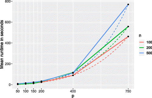
Although Lemma 4.1 gives the computational complexity of one iteration of the algorithm, numerical experiments indicate that the method converges in small number of steps, indicating that the complexity of Algorithm 1 is approximately the same; see Figure 1.

Fig. 1 Mean runtime (in seconds) over 50-runs of MRCT algorithm for Model 2 in simulation study 5, for the sample size $n=100,200,500$, as a function of a number of the observed time points $p=50,100,150,200,400,750$. Dotted lines represent the fitted cubic curve to the mean runtime as a function of p.

4.3 Selection of the Regularization Parameter α and the Subset Size h

Remark 3.1 argues that the use of the trace of the covariance of non-standardized observations as an objective results in spherically-biased subsets, where such an obstacle is mitigated by first standardizing the multivariate data so that the obtained covariance is proportional to the identity. As no random function in $L_2(I)$ has an identity covariance, the approach is to choose α such that the eigenvalues of $C(X_{\text{st}}^{\alpha })$ are either as close to 0 (for the lower part of the spectrum), or as close to some nonzero value, making them also mutually as close together as possible (for the upper part of the spectrum). The approach amounts to minimizing the noise in the data, while at the same time making all the signal components “equally important”; for an illustration see Figure 2 in the supplement. On the sample level, for fixed $\alpha >0$ and the robust estimate of the covariance $k_{H_0}{\widehat{C}}_{H_0}(X_{\text{st},H_0}^{\alpha ,k_{H_0}})$, we first calculate ${\widehat{\lambda }}_{i,\text{st},H_0}^{\alpha }={(k_{H_0}{\widehat{\lambda }}_{i,H_0})}^2/{(k_{H_0}{\widehat{\lambda }}_{i,H_0}+\alpha )}^2$, where ${\widehat{\lambda }}_{i,H_0}$ is the ith eigenvalue of ${\widehat{C}}_{H_0}(X_{\text{st},H_0}^{\alpha ,k_{H_0}})$, $i=1,\dots ,p$. Next, we search for a partition $\{S_1^{\alpha },S_2^{\alpha }\},S_1^{\alpha }\cup S_2^{\alpha }=\{1,\dots ,p\},S_1^{\alpha }\cap S_2^{\alpha }=\varnothing$, such that $$\{S_1^{\alpha },S_2^{\alpha },c_{S_1^{\alpha }}\}=\text{arg} {\mathrm{\text{min}}}_{\begin{array}{c}\{A_1,A_2,c_{A_1}\}:c_{A_1}>0,\mathrm{ }{A}_1\cup A_2\hfill \\ \mathrm{\hspace{1em}}\mathrm{\hspace{1em}}=\{1,\dots ,p\},\mathrm{ }{A}_1\cap A_2=\varnothing \hfill \end{array}}V(A_1;c_{A_1})+V(A_2;0),$$where $V(A_1;c_{A_1})=\sum _{i\in A_1}{({\widehat{\lambda }}_{i,\text{st},H_0}^{\alpha }-c_{A_1})}^2,V(A_2;0)=\sum _{i\in A_2}{({\widehat{\lambda }}_{i,\text{st},H_0}^{\alpha })}^2$. Observe first that as ${\widehat{\lambda }}_{1,H_0}\ge {\widehat{\lambda }}_{2,H_0}\ge \cdots$, and due to the monotonicity of $x\mapsto x^2/{(x+\alpha )}^2$, ordering is preserved for the standardized eigenvalues. $\text{tr}({\widehat{C}}_{H_0})<\infty$, giving $\sum _{i\ge 1}{\widehat{\lambda }}_{i,H_0}^4\le \infty$, and further implying $\sum _{i\ge 1}{({\widehat{\lambda }}_{i,\text{st},H_0}^{\alpha })}^2<0$ and $\underset{i\to \infty }{\mathrm{\text{lim}}}{({\widehat{\lambda }}_{i,\text{st},H_0}^{\alpha })}^2\to 0$. Thus, for any $c_{A_1}>0$, there exists $i_0\in \mathbb{N}$, such that ${({\widehat{\lambda }}_{i,\text{st},H_0}^{\alpha }-c_{A_1})}^2>{({\widehat{\lambda }}_{i,\text{st},H_0}^{\alpha })}^2$, implying that the set S₁ is finite, and the problem of finding an optimal partition amounts to finding $m_{\alpha }>0$ such that $$\begin{array}{c}{m}_{\alpha }=\text{arg} {\mathrm{\text{min}}}_{m>0}V\left(\{1,\dots ,m\};\frac{1}{m}\sum _{i=1}^m{\widehat{\lambda }}_{i,\text{st},H_0}^{\alpha }\right)\\ \hspace{1em}+V\left(\left\{m+1,m+2,\dots \right\};0\right).\end{array}$$

Fig. 2 A typical trajectory of the objective for selecting α for Model 1 $(n=200,p=100,c=0.2)$ in the simulation study in Section 5 (left). The objective in (9) as a function of subset size $n/2\le h\le n$, corresponding to the setting on the left and $\alpha \approx 0.6$. A sudden increase around h = 160, caused by the first outliers being included in the subset.

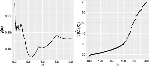
Finally, we search for $\alpha \in \text{arg} \mathrm{\text{min}}g(\alpha )$, where (10) $$\begin{array}{c}g(\alpha )=(V(\{1,\dots ,m_{\alpha }\};\frac{1}{m}\sum _{i=1}^m{\widehat{\lambda }}_{i,\text{st},H_0}^{\alpha })+V(\{m_{\alpha }+1,\dots \};0))\\ \hspace{1em}\times {(\frac{1}{m}\sum _{i=1}^m{\widehat{\lambda }}_{i,\text{st},H_0}^{\alpha })}^{-2}\end{array}$$(10) see left plot of Figure 2 for illustration.

The approach is to optimize g iteratively starting with an initial value of α₀. For an initial α₀, robust estimates of eigenvalues of C are calculated and the value of the objective function g is approximated for each α considered in the optimization. The optimal α found that way is then used for re-estimation of the robust eigenvalues of C. The following proposition establishes continuity of the Algorithm 1 w.r.t. α, reassuring that the optimization of (10) over the discrete grid yields notably effective results. More specifically, for ${\alpha }_1,{\alpha }_2$ close enough (so that the ordering of the Mahalanobis distances in STEP 8 of Algorithm 1 is preserved), given the same initial estimate H₀, using either α₁ or α₂ produces the same updated subset H₁.

Proposition 4.2.

Let $X\in L^2(I)$, and let $k_{H_0}{\widehat{C}}_{H_0}$ and ${\overline{X}}_{H_0}$ be the H₀-subset sample estimators of the covariance operator C and mean μ = 0, respectively. Then, for every $\epsilon >0$, there exists $\delta >0$, such that for ${\alpha }_1,{\alpha }_2>0,|{\alpha }_1-{\alpha }_2|<\delta ,|\Vert X_{\text{st},H_0}^{{\alpha }_1,k_{H_0}}\Vert -\Vert X_{\text{st},H_0}^{{\alpha }_2,k_{H_0}}\Vert |<\epsilon$.

The process is repeated until convergence; for more technical details see Algorithm 2 in the supplement. In the simulation study (Section 5) we use the initial ${\alpha }_0=0.01$ for p < n (see simulation study in Berrendero, Bueno-Larraz, and Cuevas (2020) for more insight), and ${\alpha }_0=1$, for p > n, emphasizing that we noticed how the initial value of α₀ has little to no effect on the output of Algorithm 2. For the sake of the numerical stability of the procedure, the additional constraint is posed on α, ensuring that the condition number of ${\widehat{C}}_{H_0}+\alpha I$ is smaller than 100; for more insight see Boudt et al. (2020).

Finally, we provide some thoughts about the choice of the subset size h. It is clear that the number of contaminated samples should be smaller than n–h, and that h should at least be $n/2$ to obtain a fit to the data majority. Therefore, the choice of h is a tradeoff between the robustness and efficiency of the estimator; see discussion in Rousseeuw (1984) for more details. In practice, the proportion of outliers is, in general, not known in advance, and thus we consider a data-driven approach for the choice of h, as suggested by Boudt et al. (2020): one considers a range of possible values for h to search for significant changes of the computed value of the objective function or the estimate. Big shifts in the norm of the difference between the subsequent covariance estimates, as well as those in the value of the trace of the corresponding covariance based on the consecutive subset sizes, can imply the presence of outliers; see the right plot of Figure 2 for illustration.

5 Simulation Study

This section evaluates the MRCT Algorithm 1 through a simulation study similar to those in Berrendero, Bueno-Larraz, and Cuevas (2020) and Arribas-Gil and Romo (2014). The methods compared to MRCT fall into three categories: those relying on functional depths, employing functional principal components, and based on the Mahalanobis distance and its functional extension. Supplementary materials and referenced works provide a detailed explanation.

In the simulation, we generate the contaminated data Y(t), $t\in (0,1)$ using Huber’s ε-contamination model Huber (1964) as $Y(t)=(1-u)X_1(t)+u{X}_2(t)$, where $u\sim \mathit{\text{Bernoulli}}(c)$, and contamination rate $c\in \{0,0.05,0.1,0.2\}$. As we observe no significant difference in the results with respect to c, due to the page limit, we present the results only for c = 0.2. The main process X₁ and the contamination X₂ are random processes chosen according to three different models to accommodate various outlier settings: $$\begin{array}{c}\mathtt{\text{Model}}\hspace{0.17em}\mathtt{1}:X_1(t)=30t{(1-t)}^{1.5}+{\epsilon }_1(t),\\ X_2(t)=30t^{1.5}(1-t)+{\epsilon }_2(t),\\ \mathtt{\text{Model}}\hspace{0.17em}\mathtt{2}:X_1(t)=4t+{ϵ}_1(t),\\ X_2(t)=4t+{(-1)}^{u}1.8+{(0.02\pi )}^{-0.5}\\ \hspace{0.17em}\mathrm{\text{exp}}\hspace{0.17em}\left(\frac{-{(t-\mu )}^2}{0.02}\right)+{ϵ}_2(t),\\ \mathtt{\text{Model}}\hspace{0.17em}\mathtt{3}:X_1(t)=4t+{ϵ}_1(t),\\ X_2(t)=4t+2\hspace{0.17em}\mathrm{\text{sin}}\hspace{0.17em}(4(t+\mu )\pi )+{ϵ}_2(t),\end{array}$$where ${\epsilon }_i$, ϵ_i, i = 1, 2 are mutually independent Gaussian random processes with zero mean and covariance functions $\gamma (s,t)=0.3\hspace{0.17em}\mathrm{\text{exp}}\hspace{0.17em}(-{0.3}^{-1}|s-t|)$ and $\gamma (s,t)=\hspace{0.17em}\mathrm{\text{exp}}\hspace{0.17em}(-|s-t|)$, respectively, and $u\sim \mathit{\text{Bernoulli}}(0.5),\mu \sim \mathcal{U}[0.25,0.75]$ are mutually independent, and independent of ${ϵ}_1,{ϵ}_2$. 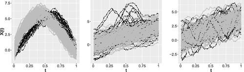For each model, we generate a random sample of n = 200 observations, with the observations recorded at an equidistant grid on the interval $[0,1]$, at p = 100 and p = 500 time points. In the context of multivariate statistics, these are referred to as low- and high-dimensional settings, respectively. Figure 3 provides a visual representation of the simulated data.

Fig. 3 Left to right, samples from Model 1,2, and 3. Solid curves represent the main processes, while the dashed ones indicate the outliers. The contamination rate is c = 0.1, sample size n = 200, and p = 100 time points.

An observation is considered an outlier if its robust α-Mahalanobis distance exceeds the cutoff value derived from the 97.5% quantile of the limiting distribution of these distances, assuming Gaussianity (Corollary 3.1). To estimate this quantile, we conduct a Monte Carlo simulation with 2000 repetitions. To measure the accuracy of the robust covariance estimator, we use the approximation of integrated square error (ISE) and the average cosine of an angle between the first 5 corresponding eigenfunctions of the estimates and true covariances (COS ${}_{1:5}$). More specifically, given the sample estimate ${\widehat{v}}_{\mathit{\text{reg}}}$ of the covariance function γ of the non-contaminated process $\text{ISE}=p^{-2}{\sum }_{i,j=1}^p(\gamma (t_i,t_j)-{\widehat{v}}_{\mathit{\text{reg}}}(t_i,t_j){)}^2$. For each method, ${\widehat{v}}_{\mathit{\text{reg}}}$ is a sample covariance estimator calculated at the identified non-outliers. Denoting ψ_i, ${\widehat{\psi }}_{\mathit{\text{reg}},i},i=1,\dots ,5$, to be the ith eigenfunction of the population covariance C and the estimated covariance ${\widehat{C}}_{\mathit{\text{reg}}}$, respectively, where the estimated covariance is based on the identified regular observations, COS ${}_{1:5}=5^{-1}{\sum }_{i=1}^5{\hspace{0.17em}\mathrm{\text{COS}}\hspace{0.17em}}_i$, where COS ${}_i=\frac{\left|{\sum }_{j=1}^p{\psi }_i(t_j){\widehat{\psi }}_{\mathit{\text{reg}},i}(t_j)\right|}{\sqrt{{\sum }_{j=1}^p{\psi }_i{(t_j)}^2{\sum }_{j=1}^p{\widehat{\psi }}_{\mathit{\text{reg}},i}{(t_j)}^2}}$. 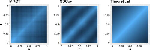Figure 4 showcases heatmaps of the estimated covariances based on MRCT and SSCov, as well as the true covariance.

Fig. 4 Left to right: heatmaps of the covariance based on the MRCT estimator, the spatial sign covariance matrix, and the true (theoretical) covariance for n = 200 observations on p = 500 time points for Model 3 with a contamination rate of 20%.

The results for the Gaussian process are depicted in Figure 5, while the analogous results for the white noise, t₃, and t₅ distributed processes (for more details see e.g., Bånkestad et al. 2020) are shown in supplement Figures 6–8. Classification rates for the outlier detection for all settings can be found in Figures 9–12 in the supplement. Additionally, we conducted a simulation study to assess computation times for the considered methods. Results are depicted in supplement Figure 13.

Fig. 5 ISE on a log-scale (top) and COS ${}_{1:5}$ (bottom). The estimates of covariance are based on identified regular observations for $n=200,p=100,500$, and c = 0.2. A solid horizontal line indicates the mean ISE for the sample covariance based on known regular observations as a reference.

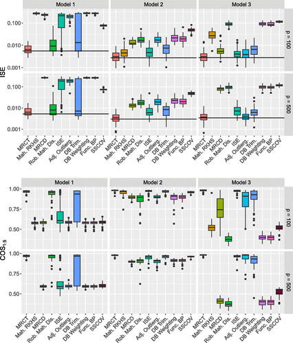
Fig. 6 SST of the Niño 1 + 2 region in the Pacific Ocean. Smoothened regular observations are depicted in gray, while outliers are represented by colored markers. The black dots in the right figure indicate the specific points in time when El Niño events were detected solely using past information, excluding 1982–1984 for the lack of past information.

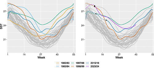
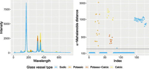
Fig. 7 Left: Spectrum of different glass vessel types. Right: Robust α-Mahalanobis distance on a log-scale. The horizontal line indicates the theoretical cutoff value.

6 Real Data Examples

6.1 Sea Surface Temperatures

The algorithm is applied to two real-world datasets, starting with an example of the El Niño-Southern Oscillation (ENSO) phenomenon in the equatorial Pacific Ocean. ENSO involves ocean surface warming known as El Niño and cooling known as La Niña, impacting global weather (Trenberth 1997). The Oceanic El Niño Index (ONI) identifies ENSO events using 3-month sea surface temperature means. For analysis, the Niño 1 + 2 region near South America is considered, using weekly sea surface temperature (SST) data from March 1982 to February 2023, resulting in a 41 × 53 data matrix sourced from https://www.cpc.ncep.noaa.gov/data/indices/. The objective is to identify atypical behavior in the yearly sea surface temperature, indicating the presence of an El Niño event. The regularization parameter $\alpha =0.271$ is selected using Algorithm 2 in the supplement. The subset size h is fixed at $\lceil 0.5n\rceil$. The identified outliers are depicted in Figure 6, and correspond to the seasons of 1982/83, 1983/84, 1997/98, 1998/99, and 2015/16. These seasons are associated with some of the strongest El Niño events, and align with findings from referenced methods such as Huang and Sun (2019) and Suhaila (2021).

The dataset was additionally supplied to the other methods from Section 5. Depth-based trimming and weighting, and the robust Mahalanobis distance find the same periods to be outlying as the MRCT. The functional boxplot and the MRCD detect 1983/84 and 1997/98, the integrated square error detects 1983/84 and 1998/99, while the adjusted outliergram only detects 1983/84 to be outlying.

We examine the possibility of forecasting them using past-year data. Our analysis involves 46 datasets: first, focusing on the initial 8 weeks (March–April), and then expanding to include additional weeks. Specifically concentrating on post 1982 episodes: 1997/98, 1998/99, and 2015/16, we handle limited data by employing smoothing techniques; see Section 4.1, using up to 15 B-spline basis functions, adjusted according to available weeks.

The findings in Figure 6 display results obtained from analyzing smoothed data. For the 1997/98 episode, the outlying behavior emerges in early May, marked by a black dot and leading to a change in curve style. Analyzing the initial 8 weeks’ temperatures promptly identifies 1998/99 observations as outliers due to sustained above-average sea surface temperatures. The 2015/16 El Niño exhibits distinct patterns, thus, being identified as an outlier by the end of June. Additionally, an investigation of the current season, 2023/24, was conducted. Using the first three quarters of data available for all years, indications point to an impending El Niño event. This is represented by the purple curve in Figure 6.

6.2 EPXMA Spectra

The dataset comprises electron probe X-ray microanalysis (EPXMA) spectra of various glass vessel types, with the objective of studying the production and trade relationships among different glass manufacturers (Janssens et al. 1998). A total of 180 observations were recorded for 1920 wavelengths. Our focus is on the first 750 time points, as they encapsulate the primary variability within the data. The data comprises four distinct types of glass vessels. The primary group, referred to as the “sodic” group, encompasses 145 observations. The remaining three groups are denoted as “potassic,” “potasso-calcic,” and “calcic,” consisting of 15, 10, and 10 measurements, respectively. Further investigation revealed that some of the spectra within the sodic glass vessels were recorded under different experimental conditions. More details regarding the different glass types can be found in Lemberge et al. (2000). The corresponding curves are depicted in the left plot of Figure 7.

For this analysis, we consider the sodic group (excluding the last 38 deviating trajectories) as the reference, and consider the remaining curves outliers. The subset size h is set to $\lceil 0.5n\rceil$ and the regularization parameter α is chosen using Algorithm 2, resulting in $\alpha =0.036$. In Figure 7 (right), robust α-Mahalanobis distances are visualized, with color indicating the data’s group structure. The vertical black line represents the theoretical cutoff Corollary 3.1. This analysis successfully pinpointed outliers in the second, third, and fourth group, as well as in the curves from the reference group following the measuring device change.

Table 1 presents outlier detection results for the methods in the simulation study, excluding Adjusted Outliergram and MRCD due to numerical issues. Integrated square error closely aligns with MRCT’s performance, while robust Mahalanobis distance and depth-based weighting seem overly conservative, leading to missed outliers as observed in the simulation study. The table also shows counts of outlying observations per group, highlighting instances where methods miss-classified observations due to cutoff extremes.

Table 1 True positive and true negative rates for different methods as well as the number of observations considered outlying within the each group.

Method	TPR	TNR	Observations considered outlying
			reg. Sodic	irreg. Sodic	Potassic	Potasso-Calcic	Calcic
Func. BP	1	0	107	38	15	10	10
Rob. Mah. Dis.	0	1	0	0	0	0	0
ISE	0.95	0.80	21	38	11	10	10
DB Trim.	0.50	0.99	1	5	14	8	10
DB Weighting	0.01	1	0	1	0	0	0
MRCT	1	0.99	1	38	15	10	10

7 Summary and Conclusions

In this article, we presented the minimum regularized covariance trace (MRCT) estimator, a novel method for robust covariance estimation and functional outlier detection. To handle outlying observations, we adopted a subset-based approach that favors the subsets that are the most central w.r.t the corresponding covariance, and where the centrality of the point is measured by the α-Mahalanobis distance (3.1) Berrendero, Bueno-Larraz, and Cuevas (2020). The approach results with the fast-MCD Rousseeuw and Driessen (1999) type algorithm, in which the notion of standard Mahalanobis distance is replaced by α-Mahalanobis distance. Consequentially, the robust estimator of the α-Mahalanobis distance is obtained, thus, further allowing for robust outlier detection. The method automates outlier detection by providing theoretical cutoff values based on additional distributional assumptions. An additional advantage of our approach is its ability to handle datasets with a high number of observed time points ($p\gg n$) without requiring preprocessing or dimension reduction techniques such as smoothing. This is a consequence of the fact that the $X_{\text{st}}^{\alpha }$ is a smooth approximation (obtained via the Tikhonov regularization) of the solution Y of the ill-posed linear problem $C^{1/2}Y=X$, where the amount of smoothening is determined by a (univariate) regularization parameter $\alpha >0$. Therefore, a certain amount of smoothening is in fact done within the procedure itself. Additionally, the selection of the regularization parameter α is automated to obtain a balance between noise exclusion and preservation of signal components.

As a part of future research, we will study the behavior and efficacy of different variants of Tikhonov regularization. While our article focused on the “standard form” with a simple smoothness penalty of $\alpha \left|\right|Y|{|}^2$, future investigations could encompass a broader scope of penalizations of the form $\alpha \left|\right|\mathit{\text{LY}}|{|}^2$, where L represents a suitable regularization operator; see for example Golub, Hansen, and O’Leary (1999). Another avenue for exploration lies in extending the approach to accommodate the case of multivariate functional data.

Supplementary Materials

The supplementary materials consist of five sections. Sections A and B cover preliminary results in Functional Data Analysis (FDA), and additional findings not presented in the main text. Section C and D provide extra simulation results and algorithmic routines, respectively. Section E comprises the proofs. The R-code for reproducing the shown results is also available in the supplementary materials.

Disclosure Statement

The authors report there are no competing interests to declare.

Additional information

Funding

This research was funded in whole or in part by the Austrian Science Fund (FWF) [10.55776/I5799]. For open access purposes, the author has applied a CC BY public copyright license to any author accepted manuscript version arising from this submission.

References

- Arribas-Gil, A., and Romo, J. (2014), “Shape Outlier Detection and Visualization for Functional Data: The Outliergram,” Biostatistics, 15, 603–619. DOI: 10.1093/biostatistics/kxu006.
- Basna, R., Nassar, H., and Podgórski, K. (2022), “Data Driven Orthogonal Basis Selection for Functional Data Analysis,” Journal of Multivariate Analysis, 189, 104868. DOI: 10.1016/j.jmva.2021.104868.
- Berkey, C. S., Laird, N. M., Valadian, I., and Gardner, J. (1991), “Modelling Adolescent Blood Pressure Patterns and their Prediction of Adult Pressures,” Biometrics, 47, 1005–1018.
- Berrendero, J. R., Bueno-Larraz, B., and Cuevas, A. (2020), “On Mahalanobis Distance in Functional Settings,” Journal of Machine Learning Research, 21, 1–33.
- Billor, N., Hadi, A., and Velleman, P. (2000), “Bacon: Blocked Adaptive Computationally Efficient Outlier Nominators,” Computational Statistics and Data Analysis, 34, 279–298. DOI: 10.1016/S0167-9473(99)00101-2.
- Blei, D. M., Kucukelbir, A., and McAuliffe, J. D. (2017), “Variational Inference: A Review for Statisticians,” Journal of the American Statistical Association, 112, 859–877. DOI: 10.1080/01621459.2017.1285773.
- Bånkestad, M., Sjölund, J., Taghia, J., and Schön, T. (2020), “The Elliptical Processes: A Family of Fat-Tailed Stochastic Processes,” arXiv preprint arXiv:2003.07201.
- Boente, G., and Salibián-Barrera, M. (2021), “Robust Functional Principal Components for Sparse Longitudinal Data,” METRON, 79, 159–188. DOI: 10.1007/s40300-020-00193-3.
- Boudt, K., Rousseeuw, P. J., Vanduffel, S., and Verdonck, T. (2020), “The Minimum Regularized Covariance Determinant Estimator,” Statistics and Computing, 30, 113–128. DOI: 10.1007/s11222-019-09869-x.
- Castro, P. E., Lawton, W. H., and Sylvestre, E. A. (1986), “Principal Modes of Variation for Processes with Continuous Sample Curves,” Technometrics, 28, 329–337. DOI: 10.2307/1268982.
- Cucker, F., and Zhou, D. X. (2007), Learning Theory: An Approximation Theory Viewpoint, Cambridge Monographs on Applied and Computational Mathematics, Cambridge: Cambridge University Press.
- Cuevas, A., Febrero, M., and Fraiman, R. (2007), “Robust Estimation and Classification for Functional Data via Projection-based Depth Notions,” Computational Statistics, 22, 481–496. DOI: 10.1007/s00180-007-0053-0.
- Ding, J., and Zhou, A. (2007), “Eigenvalues of Rank-One Updated Matrices with Some Applications,” Applied Mathematics Letters, 20, 1223–1226. DOI: 10.1016/j.aml.2006.11.016.
- Eilers, P. H. C., and Marx, B. D. (1996), “Flexible Smoothing with B-splines and Penalties,” Statistical Science, 11, 89–121. DOI: 10.1214/ss/1038425655.
- Ferraty, F., and Vieu, P. (2007), “Nonparametric Functional Data Analysis: Theory and Practice,” Computational Statistics & Data Analysis, 51, 4751–4752.
- Gervini, D. (2008), “Robust Functional Estimation Using the Median and Spherical Principal Components,” Biometrika, 95, 587–600. DOI: 10.1093/biomet/asn031.
- Golub, G. H., Hansen, P. C., and O’Leary, D. P. (1999), “Tikhonov Regularization and Total Least Squares,” SIAM Journal on Matrix Analysis and Applications, 21, 185–194. DOI: 10.1137/S0895479897326432.
- Huang, H., and Sun, Y. (2019), “A Decomposition of Total Variation Depth for Understanding Functional Outliers,” Technometrics, 61, 445–458. DOI: 10.1080/00401706.2019.1574241.
- Huber, P. J. (1964), “Robust Estimation of a Location Parameter,” The Annals of Mathematical Statistics, 35, 73–101. DOI: 10.1214/aoms/1177703732.
- Hubert, M., Rousseeuw, P. J., and Verdonck, T. (2012), “A Deterministic Algorithm for Robust Location and Scatter,” Journal of Computational and Graphical Statistics, 21, 618–637. DOI: 10.1080/10618600.2012.672100.
- Janssens, K. H., Deraedt, I., Schalm, O., and Veeckman, J. (1998), “Composition of 15–17th Century Archaeological Glass Vessels Excavated in Antwerp, Belgium,” in Modern evelopments and Applications in Microbeam Analysis, eds. G. Love, W. A. P. Nicholson, and A. Armigliato, pp. 253–267, Vienna: Springer.
- Kokoszka, P., and Reimherr, M. (2017), Introduction to Functional Data Analysis, Chapman & Hall/CRC Numerical Analysis and Scientific Computing, Boca Raton, FL: CRC Press.
- Kullback, S. (1959), Information Theory and Statistics, New York: Wiley.
- Kullback, S., and Leibler, R. A. (1951), “On Information and Sufficiency,” The Annals of Mathematical Statistics, 22, 79–86. DOI: 10.1214/aoms/1177729694.
- Lemberge, P., Raedt, I., Janssens, K., Wei, F., and Van Espen, P. (2000), “Quantitative Analysis of 16-17th Century Archaeological Glass Vessels Using PLS Regression of epxma and μ-xrf data,” Journal of Chemometrics, 14, 751–763. DOI: 10.1002/1099-128X(200009/12)14:5/6<751::AID-CEM622>3.0.CO;2-D.
- Locantore, N., Marron, J. S., Simpson, D. G., Tripoli, N., Zhang, J. T., Cohen, K. L., Boente, G., Fraiman, R., Brumback, B., Croux, C., Fan, J., Kneip, A., Marden, J. I., Peña, D., Prieto, J., Ramsay, J. O., Valderrama, M. J., and Aguilera, A. M. (1999), “Robust Principal Component Analysis for Functional Data,” Test, 8, 1–73. DOI: 10.1007/BF02595862.
- Ostebee, A., and Zorn, P. (2002), Calculus from Graphical, Numerical, and Symbolic Points of View. Number Bd. 2 in Calculus from Graphical, Numerical, and Symbolic Points of View. San Diego, CA: Harcourt College Publishers.
- Ramsay, J. O., and Silverman, B. W. (1997), Principal Components Analysis for Functional Data, New York: Springer.
- Rousseeuw, P. J. (1984), “Least Median of Squares Regression,” Journal of the American Statistical Association, 79, 871–880. DOI: 10.1080/01621459.1984.10477105.
- Rousseeuw, P. J., and Driessen, K. V. (1999), “A Fast Algorithm for the Minimum Covariance Determinant Estimator,” Technometrics, 41, 212–223. DOI: 10.1080/00401706.1999.10485670.
- Sawant, P., Billor, N., and Shin, H. (2012), “Functional Outlier Detection with Robust Functional Principal Component Analysis,” Computational Statistics, 27, 83–102. DOI: 10.1007/s00180-011-0239-3.
- Suhaila, J. (2021), “Functional Data Visualization and Outlier Detection on the Anomaly of el Niño Southern Oscillation,” Climate, 9, 118. DOI: 10.3390/cli9070118.
- Trenberth, K. E. (1997), “The Definition of el Niño,” Bulletin of the American Meteorological Society, 78, 2771–2778. DOI: 10.1175/1520-0477(1997)078<2771:TDOENO>2.0.CO;2.
- Wang, J.-L., Chiou, J.-M., and Mueller, H.-G. (2015), “Review of Functional Data Analysis,” arXiv preprint arXiv:1507.05135.
- Zhang, Y., Liu, W., Chen, Z., Wang, J., and Li, K. (2023), “On the Properties of Kullback-Leibler Divergence between Multivariate Gaussian Distributions,” arXiv preprint arXiv:2102.05485.