Detection of Emergent Anomalous Structure in Functional Data

Abstract

Motivated by an example arising from digital networks, we propose a novel approach for detecting the emergence of anomalies in functional data. In contrast to classical functional data approaches, which detect anomalies in completely observed curves, the proposed approach seeks to identify anomalies sequentially as each point on the curve is received. The new method, the Functional Anomaly Sequential Test (FAST), captures the common profile of the curves using Principal Differential Analysis and uses a form of CUSUM test to monitor a new functional observation as it emerges. Various theoretical properties of the procedure are derived. The performance of FAST is then assessed on both simulated and telecommunications data.

Keywords:

• Anomaly detection
• Emergent anomaly
• Functional Anomaly Sequential Test (FAST)
• Functional data analysis

1 Introduction

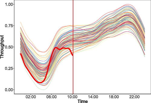
This article is motivated by a anomaly detection challenge arising from a telecommunications application monitoring throughput data at a point on a digital network. As can be seen from Figure 1(a), this data takes the form of a smooth curve that takes similar values over any given day. Following Woodall et al. (2004) we model such observations as functional data, and refer to the repeated pattern as the profile of the data. In some instances, however, there is a deviation from this anticipated profile (See Figure 1(b)). We term such deviations anomalies, with these events indicating the possible occurrence of a significant event on the network that requires an operational intervention. Due to the need to perform the operational intervention as soon as possible we ideally need a method that is able to sequentially monitor an incomplete profile for anomalies as they emerge, that is as each point on the profile is received (See Figure 2).

Fig. 1 Observations of throughput data recorded at 1 min intervals over 100 days at a point on a telecommunications network and represented as a functional time series. Each curve denotes a single day of data (a). An instance of an anomalous day is overlaid in red in (b).

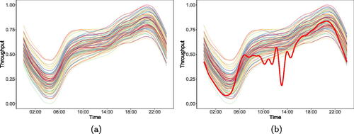
Fig. 2 Example showing the emergence of an anomaly (bolded line) within the functional data from Figure 1(b). The solid vertical line indicates the time by which the anomaly can be said to have emerged, and it is desirable to detect this event as quickly as possible.

Adopting the terminology of Dai et al. (2020), in a functional data setting an observed profile may contain either a magnitude or a shape anomaly. A magnitude anomaly is a curve that is outlying when compared to the rest of the sample, whereas a shape anomaly has a different shape from the rest of the sample despite not being an outlier. The current state-of-the-art for functional anomaly detection has focused on identifying these anomalies within a sample of completely observed profiles, which we refer to as the offline setting. Figure 1(b) presents an example of an offline detection problem. Various authors have considered the offline detection of shape and magnitude anomalies, including Hyndman and Shang (2010), López-Pintado and Romo (2011), Arribas-Gil and Romo (2014), Rousseeuw, Raymaekers, and Hubert (2018), Dai and Genton (2018), Huang and Sun (2019), Harris et al. (2020), and Rieser and Filzmoser (2022).

A related challenge to offline functional anomaly detection, known as profile monitoring, monitors complete functional observations (the profiles) as they are received sequentially (Woodall 2007). At each time step the set of profiles received so far are then compared to a non-anomalous baseline profile to determine if there has been a sustained change. In contrast to offline anomaly detection, in which an anomaly consists of a single profile that differs from the others in the sample, this sustained change means that all future profiles that are received now differ from the originally observed baseline. Existing profile monitoring techniques include those of Hall, Poskitt, and Presnell (2001), Jeong, Lu, and Wang (2006), Colosimo and Pacella (2010), Paynabar, Zou, and Qiu (2016), Yan, Paynabar, and Shi (2018), and Flores et al. (2020).

Recalling the key requirement of our motivating application, that data are monitored sequentially to identify the emergence of an anomaly, we see that the aforementioned approaches are not suitable for this setting. Specifically, offline functional anomaly detectors cannot be applied because they need a profile to be completely observed. Existing profile monitoring techniques, on the other hand, are unsuitable because they are searching for a changepoint in a sequence of functional profiles rather than identifying individual anomalies. As an alternative, a nonfunctional data approach for monitoring nonstationary data could be applied, for example Zhang, Mei, and Shi (2018), Wang et al. (2018), or Talagala et al. (2020). These techniques are also inappropriate for our setting, however, because they are not designed to handle the temporal dependence contained in functional data and require anomalies that consist of an abrupt change in a parameter such as the mean.

To address the shortcomings in the existing literature we propose detecting deviations from a functional profile sequentially, as each point on the profile is received. To this end we introduce a Functional Anomaly Sequential Test (FAST). The essence of our proposed approach can be summarized as follows: FAST first estimates the best fitting linear differential operator from a set of training data, before then applying this operator to a new observation to obtain a new estimated residual function. This residual function is used to calculate the test statistic for a nonparametric CUSUM test (Tartakovsky, Rozovskii, and Shah 2005), where if the cumulative value of this test statistic exceeds a threshold then an anomaly is declared. By performing this CUSUM test sequentially on a partially observed curve anomalies can be detected as they emerge.

The remainder of the article is organized as follows: Section 2 introduces the functional data framework and methodology that underpins the FAST procedure. Various theoretical properties of the anomaly detection procedure are established in Section 3, including a threshold that controls the false alarm rate, and results relating to the power of the test. A simulation study is then described in Section 4, illustrating the performance of the method across a range of settings. We conclude in Section 5 with an analysis of the throughput telecommunications data.

2 Background and Methodology

We start by outlining our approach to detecting emergent anomalies in functional data. In Sections 2.1 and 2.2 we introduce the model which we assume describes the data observed and our estimation approach, prior to introducing the FAST algorithm in Section 2.3.

2.1 Model

In what follows we adopt the functional data model of Ramsay (2005). Consider a sequence of functional observations $\left\{X_1(t),X_2(t),\dots ,X_n(t)\right\}\in L^2(\mathcal{T})$, none of which are anomalous, and where the subscript denotes the ith observation over the interval $\mathcal{T}$. In this work the interval is a day, so it is convenient to view $\left\{X_i(t)\right\}$ as denoting the observed value for the ith day at time t.

As described in Section 1, each of our non-anomalous observations follows an underlying profile. In order to represent this underlying structure we use the approach of Ramsay (2005) and model the observations as noisy realizations of the solution to an order m linear ODE, with the solution to the ODE describing the underlying profile structure. The linear operator, $\mathcal{L}$, for this ODE takes the following form: (1) $$\mathcal{L}={\beta }_0(t){\mathrm{D}}^0+{\beta }_1(t)\mathrm{D}+\cdots +{\beta }_{m-1}(t){\mathrm{D}}^{m-1}+{\mathrm{D}}^m,$$(1) where D^k denotes the kth derivative of a function, and the ${\left\{{\beta }_j(t)\right\}}_{j=0}^{m-1}$ are coefficient functions that are estimated from the data. The estimation of $\mathcal{L}$, and the choice of m, will be discussed in the next section.

Under the assumption that each observation is a noisy realization of the solution to the ODE in (1), an observation is given by (2) $$X_i(t)=\sum _{j=1}^m{c}_j{u}_j(t)+f_i(t),\hspace{1em}{c}_j\in \mathbb{R},1\le i\le n,t\in \mathcal{T}.$$(2)

Here ${\left\{u_j(t)\right\}}_{j=1}^m$ are the solutions to the ODE in (1), and ${\sum }_{j=1}^m{c}_j{u}_j(t)$ represents the underlying profile for the data. In (2) it is assumed that the $\left\{u_j(t)\right\}$ are linearly independent m-times differentiable functions, and the $\left\{f_i(t)\right\}$ are m-times differentiable mean-zero functional random variables representing noise.

We make the following assumption about the noise functions:

Assumption 1.

The noise functions, $\left\{f_i(t)\right\}$, are independent mean zero Gaussian processes with stationary covariance functions.

Although FAST does not require this assumption to work in practice, it is used for model selection in Section 2.2, and to develop an asymptotic distribution for the test statistic in Section 3.

The aim of FAST is to detect when an observation has been contaminated by an anomaly. We model an anomaly as a function, $\left\{g_i(t)\right\}$, causing a deviation from the underlying profile for the data. We make the following assumptions regarding these anomaly functions:

Assumption 2.

The anomaly functions $\left\{g_i(t)\right\}$ are (i) m-times differentiable, and (ii) not equal to a linear combination of the $\left\{u_j(t)\right\}$.

Assumption 2(i) is required so that the differentiability condition on the $\left\{X_i(t)\right\}$ is still satisfied when an anomaly is present. Additionally, Assumption 2(ii) ensures that the anomaly does not follow the underlying profile for the data. We also remark that it is not necessary for an anomaly function to contaminate the entire observation period, and that it can be present on some sub-region, $\mathcal{S}\subset \mathcal{T}$.

Building on (2), a model for a contaminated observation can be defined as (3) $$X_i(t)=\{\begin{array}{cc}\sum _{j=1}^m{c}_j{u}_j(t)+f_i(t)& t\in \mathcal{T}\setminus {\mathcal{S}}_i\\ \sum _{j=1}^m{c}_j{u}_j(t)+f_i(t)+g_i(t)& t\in {\mathcal{S}}_i.\end{array}$$(3)

While the above functional data model for the observations assumes continuous time, this may not be possible in practice. In such circumstances we follow the approach taken by other authors such as Nagy, Gijbels, and Hlubinka (2016), and model the observations on a fine grid. We let $\left\{1,\dots ,T\right\}$ be the fine grid that discretizes the compact set $\mathcal{T}$, and let the discretized observation be denoted by ${\left\{X_i(\tau )\right\}}_{\tau =1}^T$ for $1\le i\le n$.

With our model for the data generating process outlined, we now turn to consider the estimation scheme that will be used. As we shall see in Section 2.3, the FAST algorithm uses an estimate of the differential operator in (1), rather than estimates of the solution functions in (2). To estimate the operator, we follow the approach of Ramsay (1996) and use Principal Differential Analysis, as we describe in the next section.

2.2 Estimating the Model Using Principal Differential Analysis

We begin by recalling that the approach of Ramsay (1996) to estimating a linear differential operator to model functional data uses Principal Differential Analysis (PDA). PDA estimates the best fitting order m linear differential equation for a sample of functional data. As described in the previous section, in this work the linear differential operator takes the form of (1).

Following Ramsay (1996), an estimate for $\mathcal{L}$ can be obtained by selecting the values of $\mathit{\beta }(\mathit{t})={\left\{{\beta }_j(t)\right\}}_{j=0}^{m-1}$ that minimize ${\sum }_{i=1}^n\left|\right|\mathcal{L} (X_i(t))|{|}_2^2={\sum }_{i=1}^n{\sum }_{\tau =1}^T\mathcal{L} {(X_i(\tau ))}^2$. The estimated differential operator, $\widehat{\mathcal{L}}$, will have m linearly independent solutions, and these estimated solution functions are estimates of $\left\{u_j(t)\right\}$ in (2).

To detect anomalies the FAST algorithm applies the estimated differential operator to the observed data. This produces a set of residual functions, ${\left\{{ϵ}_i(t)\right\}}_{i=1}^n$, and it is these residual functions that form a key part of our test. We denote the estimated residual obtained by applying the estimated operator by ${\left\{{\widehat{ϵ}}_i(t)\right\}}_{i=1}^n$. Note that under Assumption 1, and using the well known properties of Gaussian processes, the residual functions are also themselves mean-zero Gaussian processes (Rasmussen and Williams 2005).

Using the fact that the $\left\{u_j(t)\right\}$ are solutions to $\mathcal{L}$, and so $\mathcal{L}(u_j(t))=0$, an explicit connection between the residual functions and the model for the data presented in (2) is given by the following: (4) $$\begin{array}{c}\mathcal{L}(X_i(t))=\mathcal{L}\left(\sum _{j=1}^m{c}_j{u}_j(t)+f_i(t)\right)\\ =\mathcal{L}\left(f_i(t)\right)\\ ={ϵ}_i(t),\hspace{1em}1\le i\le n.\end{array}$$(4)

Although it will not be known a priori if an observation is contaminated with an anomaly, it can also be instructive to consider what happens when the differential operator is applied to such an observation. Applying the estimated operator to the model in (3) gives the following: (5) $$\mathcal{L}(X_i(t))=\{\begin{array}{cc}{ϵ}_i(t)\hfill & t\in \mathcal{T}\setminus {\mathcal{S}}_i\hfill \\ \mathcal{L}(g_i(t))+{ϵ}_i(t)\hfill & t\in {\mathcal{S}}_i.\hfill \end{array}$$(5)

It is this property that motivates the FAST test: observations that deviate from the underlying profile for the data will have contaminated residual functions.

One aspect of the model estimation that is yet to be addressed is the selection of m, the order of the ODE structure to fit to the data. This is a subject that has received little attention in the literature to date. It is suggested in Ramsay (1996) that the m should be specified by discussion with experts or through use of physical modeling. Unfortunately in many applications, for example the telecommunications example in Section 5, the order will not be known a priori.

As an alternative, we propose selecting the order of the differential operator in a data driven manner, motivated by the selection of regression models. In particular, it is proposed that the Bayesian Information Criterion (BIC) (Schwarz 1978) is used to select the order of the ODE to fit to the data (Teräsvirta and Mellin 1986). BIC is given by (6) $$\text{BIC}(m)=m\hspace{0.17em}\mathrm{\text{log}}\hspace{0.17em}(n)-2\widehat{\mathcal{l}}$$(6) where $\widehat{\mathcal{l}}$ is the log-likelihood of the fitted model at the MLE, m is the order for the ODE and n is the number of observed curves. Using Assumption 1, the residual functions are mean zero Gaussian processes, and so on a discretized grid ${\left\{{ϵ}_i(\tau )\right\}}_{\tau =1}^T$ will follow a mean zero multivariate Gaussian distribution. As such, the log-likelihood in (6) is that of a multivariate normal distribution. In the case where the noise functions are independent the log-likelihood reduces to (Johnson and Wichern 1988): (7) $$\widehat{\mathcal{l}}=-\frac{n}{2}\mathrm{\text{log}}\hspace{0.17em}(\frac{\sum _{i=1}^n\sum _{\tau =1}^T{\widehat{ϵ}}_i^2(\tau )}{n}),$$(7) where ${\sum }_{i=1}^n{\sum }_{\tau =1}^T{\widehat{ϵ}}_i^2(\tau )$ is the sum of square error between the observations and the solution to the estimated ODE. We explore the effectiveness of this approach in simulations in Section 4.4.

2.3 FAST: A Test for Intra-Functional Anomaly Detection

Having established our approach for estimating the differential operator $\mathcal{L}$ for non-anomalous data, we are in a position to introduce FAST. The aim of FAST is to sequentially monitor an emerging functional observation for anomalous behavior. To achieve this it combines the estimation step introduced in the previous section with a nonparametric CUSUM test to identify when an anomaly is emerging. The pseudocode for FAST can be found in Algorithm 1.

The first stage of the FAST algorithm takes as input a set of anomaly-free training observations, $\left\{X_1,\dots ,X_n\right\}\in L^2(\mathcal{T})$, and uses PDA to estimate $\widehat{\mathcal{L}}$. This best fitting linear differential operator is then applied to a new observation $\left\{X_{n+1}(t)\right\}$ to obtain a residual function, $\left\{{\widehat{ϵ}}_{n+1}(t)\right\}$. The residual function can then be used to define the test function, $Z_i(\tau )$, used by FAST. This is given by (8) $$Z_{n+1}(\tau )=\frac{S_{n+1}(\tau )-\mu (\tau )}{\sigma (\tau )},\hspace{1em}2\le \tau \le T$$(8) where $$S_{n+1}(\tau )={\left({\widehat{ϵ}}_{n+1}(\tau )-{\widehat{ϵ}}_{n+1}(\tau -1)\right)}^2,\hspace{1em}2\le \tau \le T.$$

Note that $\mu (\tau )$ and $\sigma (\tau )$ are the mean and standard deviation of $S_{n+1}$ at time τ, respectively. In some settings, the structure for the noise function will be known and so $\mu (\tau )$ and $\sigma (\tau )$ can be obtained analytically. In others, however, these values will be unknown. In this case they can be estimated from the training data that has been used to estimate $\widehat{\mathcal{L}}$. We then replace the $\mu (\tau )$ and $\sigma (\tau )$ in (8) with their estimators $\widehat{\mu }(\tau )$ and $\widehat{\sigma }(\tau )$.

We standardize the test function in (8) so that at each time step it is a mean-zero, unit variance random variable. This is necessary so that a threshold for the test can be derived that controls the false alarm rate when the observations are dependent, as is expected in the functional data setting. The cumulative sum of (8) can then be treated as the test statistic, ${\Delta }_{n+1}(\tau )$; this is given by (9) $${\Delta }_{n+1}(\tau )=\sum _{r=2}^{\tau }{Z}_{n+1}(r),\hspace{1em}2\le \tau \le T.$$(9)

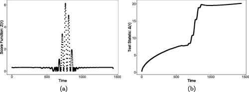
In Figure 3 we provide a plot of both $Z_{n+1}(\tau )$ and ${\Delta }_{n+1}(\tau )$ for the anomaly in Figure 1 after fitting an order 2 ODE to the non-anomalous data using PDA. Notice how, as the anomaly emerges, the values of $Z_{n+1}(\tau )$ increase, and this in turn leads to a noticeable rise in the test statistic.

Fig. 3 Figure showing the values of $Z_{n+1}(\tau )$ (a) and ${\Delta }_{n+1}(\tau )$ (b) for the anomaly in Figure 1.

When performing FAST, the absolute value of ${\Delta }_{n+1}(\tau )$ is taken so that the test is one sided. This is convenient since it allows for a single threshold for the test to be selected by a user; and also because we do not make the distinction between large positive, or negative, deviations of ${\Delta }_{n+1}(\tau )$. Furthermore, in line with the existing CUSUM literature, the test statistic is scaled by the square root of the length of the cumulative sum. The purpose of this is to control the increasing variation of the test statistic under the null as the value of T increases.

An anomaly is detected should the scaled test statistic cross a threshold denoted by $\gamma \ge 0$. This gives rise to the following stopping rule for FAST: (10) $$\xi =\mathrm{\text{min}}\left\{2\le \tau \le T:\frac{|{\Delta }_{n+1}(\tau )|}{\sqrt{\tau -1}}\ge \gamma \right\},$$(10) where $\mathrm{\text{min}}\{\varnothing \}=\infty$ indicates no alarm being sounded. The threshold, γ, is chosen so that the false alarm probability for FAST is controlled. While in practice this could be obtained through simulation, it is also possible to derive a theoretical choice for the threshold for settings where Assumption 1 holds. This choice is discussed in Section 3.

Algorithm 1:

FAST Algorithm

____________________________________________________________

Compute $\widehat{\mathcal{L}}$ from the observed data $X_1,\dots ,X_n$.;

for τ in $2:T$ do

Compute $S_1(\tau ),\dots ,S_n(\tau )$; $$\mu (\tau )=n^{-1}\sum _{i=1}^n{S}_i(\tau );$$ $$\sigma (\tau )={(n-1)}^{-1}\sum _{i=1}^n(S_i(\tau )-\mu (\tau ){)}^2;$$

end

Initialization;

Set $\Delta (1)=0$;

Choose the threshold γ;

for τ in $2:T$ do

Compute $Z_{n+1}(\tau )$; $${\Delta }_{n+1}(\tau )={\Delta }_{n+1}(\tau -1)+Z_{n+1}(\tau );$$

if $|{\Delta }_{n+1}(\tau )|\ge \gamma \sqrt{\tau -1}$ then

BREAK;

end

end

______________________________________________________________________________________________

Finally, we turn to consider the computational cost of FAST. To perform FAST the ODE operator for the data must first be estimated from a sample of n functional observations. Using PDA for this estimation stage has a one off upfront cost that is $\mathcal{O}(m^3{n}^{2}T)$ (Ramsay 1996). The coefficients obtained from this fitting procedure must then be stored, and so the storage complexity of our algorithm is $\mathcal{O}(\mathit{\text{mT}})$. Once the initial estimation phase is complete the anomaly detection procedure may commence, and this requires the test statistic to be computed. Updating the test statistic using (9) has a constant cost per iteration, however, computing (8) requires m derivatives to be evaluated and so the cost per iteration is $\mathcal{O}(m)$.

3 Theoretical Properties of FAST

We now derive various theoretical properties for FAST, including the selection of a threshold for the test that controls the false alarm rate at a suitable level, and results for the power of the test for both a finite sample setting and as $T\to \infty$.

In the classical (nonfunctional) online changepoint setting, it is common to consider the average run length to false alarm (ARL). In practice selection of the threshold for the changepoint test is made based on controlling the ARL at some pre-specified level. This is done using training data in many applications due to the complexity of the run length distribution (see Tartakovsky, Nikiforov, and Basseville (2014) for details). Within the functional data generating scenario that we consider, however, we only observe each curve at T points and so the test terminates at time T. Consequently, the following is a more appropriate quantity to consider in this setting: the probability of false alarm by time T. Below we propose a threshold that controls this quantity at a desired level.

The probability of a false alarm by time T is defined as (11) $$\begin{array}{c}\mathrm{P}(\xi \le T|\text{No Change})=\mathrm{P}\left(\underset{\tau =1}{\overset{T}{\cup }}\xi =\tau |\text{No Change}\right)\\ \le \sum _{\tau =2}^T\mathrm{P}\left(\xi =\tau |\text{No Change}\right),\end{array}$$(11) where ξ is the stopping time for the test.

To establish a suitable threshold that controls the false alarm probability, we follow Eichinger and Kirch (2018) and use a central limit argument to approximate the asymptotic distribution of the test statistic in (10). We use this approximation to select the threshold as per the following proposition. As we shall see later (Section 4.1), although this is an asymptotic bound, it also performs favorably in the finite sample setting.

Proposition 1.

Let (12) $$\gamma ={\Phi }^{-1}\left(1-\frac{\alpha }{2(T-1)}\right)$$(12) be the threshold used in the detection test, where $\Phi (·)$ is the CDF of the standard Gaussian distribution. Then, if the $\left\{f_i(t)\right\}$ are independent mean zero Gaussian processes with stationary covariance functions, the probability of a false alarm by time T is bounded above by α.

Proof.

See supplementary material. □

While control of the false alarm rate is an important component for any sequential test, theoretical guarantees for the power of the test are also desirable. In the next result we consider an anomaly function, $\left\{g_{n+1}(\tau )\right\}$, emerging at time ν, for a period of length s; and a test threshold set as in Proposition 1. Using a Central Limit Theorem approximation we can establish the following bounds on the probability of detecting this anomaly.

Proposition 2.

Let $\left\{g_{n+1}(\tau )\right\}$ be an m-times differentiable anomaly function emerging at time ν, until time $\nu +s$, and assume that it is not equal to a linear combination of the $\left\{u_j(t)\right\}$. Then if γ is set as Proposition 1 the probability of detecting an anomaly by time T is bounded above and below by (13) $$\mathrm{P}\left(\left|U_T\right|\ge \gamma \right)\le \mathrm{P}(\xi \le T)\le \sum _{\tau =2}^T\mathrm{P}\left(\left|U_{\tau }\right|\ge \gamma \right).$$(13)

Here $U_{\tau }\sim \mathrm{N}(\frac{1}{\sqrt{\tau -1}}{\sum }_{r=2}^{\tau }\frac{\lambda (r)}{\sqrt{2}},1+\frac{1}{\tau -1}{\sum }_{r=2}^{\tau }2\lambda (r)),\lambda (r)=\frac{{(\widehat{\mathcal{L}}(g_{n+1})(r)-\widehat{\mathcal{L}}(g_{n+1})(r-1))}^2}{\mu (r)},\mu (r)=\mathrm{E}{({\widehat{ϵ}}_{n+1}(r)-{\widehat{ϵ}}_{n+1}(r-1))}^2$, and $\widehat{\mathcal{L}}(g_{n+1})(r)=0$ outside of $\nu \le r\le \nu +s$.

Proof.

See supplementary material. □

Proposition 2 illustrates how, as the size of the anomaly increases, the probability of detection increases. The connection between the result and the duration of time the anomaly emerges for, s, can also be obtained by rewriting $U_{\tau }$ as follows: $$U_{\tau }\sim \{\begin{array}{cc}\mathrm{N}(0,1)\hfill & \tau <\nu \hfill \\ \mathrm{N}\left(\frac{1}{\sqrt{\tau -1}}\sum _{r=\nu }^{\tau }\frac{\lambda (r)}{\sqrt{2}},1+\frac{1}{\tau -1}\sum _{r=\nu }^{\tau }2\lambda (r)\right)\hfill & \nu \le \tau \le \nu +s\hfill \\ \mathrm{N}\left(\frac{1}{\sqrt{\tau -1}}\sum _{r=\nu }^{\nu +s}\frac{\lambda (r)}{\sqrt{2}},1+\frac{1}{\tau -1}\sum _{r=\nu }^{\nu +s}2\lambda (r)\right)\hfill & \tau >\nu +s.\hfill \end{array}$$

In other words, as the size of s increases, both the mean and variance of $U_{\tau }$ increase. Consequently, the probability of detection also increases, much as one might expect.

A further aspect of the detection test is the fact that the test threshold depends on T. The next proposition establishes that, given certain conditions on the anomaly, as $T\to \infty$ the detection of an anomaly occurs with probability one.

Proposition 3.

Let $\left\{g_{n+1}(\tau )\right\}$ be an m-times differentiable anomaly function that emerges for all $\tau \ge \nu$, where $\nu =\lfloor \mathit{\theta T}\rfloor$ and $0<\theta <1$, assume that the anomaly function is not equal to a linear combination of the $\left\{u_j(t)\right\}$, and let A be the event that

$\left\{\widehat{\mathcal{L}}(g_{n+1})(\tau )-\widehat{\mathcal{L}}(g_{n+1})(\tau -1)=0\right\}$ at most finitely many times. Then (14) $$\underset{T\to \infty }{\mathrm{\text{lim}}}\mathrm{P}\left[\xi <\infty |A,\gamma ={\Phi }^{-1}\left(1-\frac{\alpha }{2(T-1)}\right)\right]=1.$$(14)

Proof.

See supplementary material. □

Having developed theoretical results for both the control of the false alarm probability under the null, and the power of detection under the alternative, we now turn our attention to the finite sample performance of FAST.

4 Simulation Studies

In this section we consider the performance of FAST in a finite sample setting. We aim to assess FAST’s performance for a range of different anomalies, including those that do not meet the assumptions of our setting, while controlling the false alarm probability using Proposition 1. We will also consider FAST’s performance when the anomaly occurs at the start, or end, of the profile. In practice, misspecification of the ODE order may also occur, or the training data may be contaminated with anomalies, and so we therefore include simulations to explore these scenarios. We then assess the accuracy of using BIC to select the ODE order, before showcasing the performance of FAST in the offline setting, comparing it to existing state-of-the-art methods. All simulations are performed on a 1.90GHz i7-1370P Intel processor.

In the simulations that follow nine different model scenarios are considered. These are:

• Model 1: Gaussian Process No Anomalies $X_i(t)=\hspace{0.17em}\mathrm{\text{sin}}\hspace{0.17em}\left(\frac{1}{100}\mathit{\pi t}\right)+\hspace{0.17em}\mathrm{\text{cos}}\hspace{0.17em}\left(\frac{1}{100}\mathit{\pi t}\right)+f_i(t),t\in [1,500],$ where $\left\{f_i(t)\right\}$ is a Gaussian process with covariance operator given by $C(s,t)=0.3\hspace{0.17em}\mathrm{\text{exp}}\hspace{0.17em}\left(\frac{1}{2}{(\frac{s-t}{40})}^2\right)$.

• Model 2: T-Process No Anomalies $X_i(t)=\hspace{0.17em}\mathrm{\text{sin}}\hspace{0.17em}\left(\frac{1}{100}\mathit{\pi t}\right)+\hspace{0.17em}\mathrm{\text{cos}}\hspace{0.17em}\left(\frac{1}{100}\mathit{\pi t}\right)+f_i(t),$

  $t\in [1,500],$ where $\left\{f_i(t)\right\}$ is a Student’s t-process with two degrees of freedom and scale operator equal to the covariance operator in model 1.

• Model 3: Magnitude Main model: Model 1. Anomaly Model: $$g(t)=a_1+a_2\frac{t-100}{500}+a_3\hspace{0.17em}\mathrm{\text{exp}}\hspace{0.17em}\left(-\frac{(t-100)}{500}\right),a_i\sim \text{Unif}[(-0.1,-0.01)\cup (0.01,0.1)],t\in [100,200]$$

• Model 4: Random Magnitude Main model: Model 1. Anomaly Model: $g(t)=a_1+a_2\frac{t-100}{500}+a_3\hspace{0.17em}\mathrm{\text{exp}}\hspace{0.17em}(-\frac{(t-100)}{500}),a_i\sim \text{Unif}[(-0.1,-0.01)\cup (0.01,0.1)],t\in [a,b],$ $$a\sim \text{Discrete} \text{Unif}[101,491],b\sim \mathrm{\text{min}}(a+100,500).$$

• Model 5: Sinusoidal Main model: Model 1. Anomaly model: $$g(t)=b_1\left[\mathrm{\text{sin}}\hspace{0.17em}\left(\frac{2\pi t}{50}\right)-\hspace{0.17em}\mathrm{\text{sin}}\hspace{0.17em}(2\mathit{\pi t})\right]+b_2\left[\mathrm{\text{cos}}\hspace{0.17em}\left(\frac{2\pi t}{50}\right)-\hspace{0.17em}\mathrm{\text{cos}}\hspace{0.17em}(2\mathit{\pi t})\right],$$ $$b_i\sim \mathrm{U}[0.1,0.3],t\in [100,200].$$

• Model 6: Abrupt Main model: Model 1. Anomaly model: $g(t)=-\hspace{0.17em}\mathrm{\text{sin}}\hspace{0.17em}\left(\frac{1}{100}\mathit{\pi t}\right)-\hspace{0.17em}\mathrm{\text{cos}}\hspace{0.17em}\left(\frac{1}{100}\mathit{\pi t}\right),t\in [175,200]$.

• Model 7: Covariance Main model: Model 1. Anomaly model: $g(t)=-f_i(t)+\tilde{f}(t),$

  $t\in [100,200]$, where $\tilde{f}(t)$ is a Gaussian process with Covariance operator $C(s,t)=0.3\hspace{0.17em}\mathrm{\text{exp}}\hspace{0.17em}\left(\frac{1}{2}{(\frac{s-t}{35})}^2\right)$.

• Model 8: Translation Main model: Model 1. Anomaly model: $$g(t)=\left(-X(t)+X(t-a)\right)+\left(f(t)-f(t-a)\right)a\sim \text{Discrete} \text{Unif}[1,10],t\in [100,200].$$

• Model 9: Heavy Tails Main model: Model 2. Anomaly model: As in model 5.

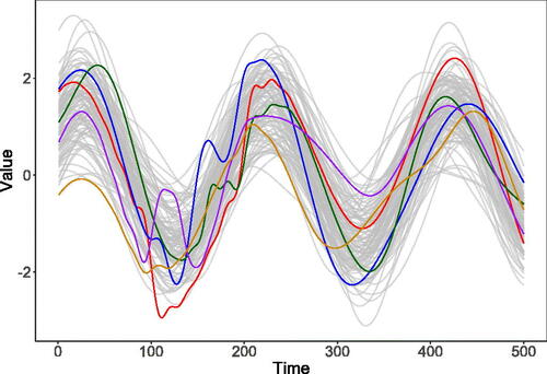
Models 1 and 2 represent two data generating processes that do not contain anomalies, and are included to assess how well Proposition 1 controls the false alarm rate both when the required assumptions are met (Model 1) and when the assumptions are not (Model 2). Models 3, 4, and 5 each contain functional magnitude anomalies with model 4 also being used to investigate how FAST is affected by the anomaly occurring at different locations in the time interval. The abrupt anomaly is a sudden change in the process to a model that only contains noise, and so during the anomalous period the profile contravenes our assumption that it can be modeled using (2). Models 7 and 8 are two examples of functional shape anomalies similar to those that have been considered by Huang and Sun (2019), with the change in covariance also illustrating how FAST performs when there is an anomaly but not a change in mean function. Finally, the purpose of model 9 is to examine detection power when the residuals are heavy-tailed. Figure 4 provides an example of the underlying process and anomaly functions. Each of the models in this section are drawn from an order m = 2 underlying profile, however, in the supplementary material we present simulations for three additional processes.

Fig. 4 This figure overlays a single instance of an anomaly from each of models 3 (red line), 5 (blue line), 6 (green line), 7 (purple line), and 8 (orange line) over 100 non-anomalous observations from model 1 (in gray). These five anomalies represent the different types of anomaly included in our simulation study, with models 4 and 9 omitted as they use the same anomaly function as models 3 and 5, respectively.

4.1 Power and Delay

We begin by exploring the detection power, and average detection delay (ADD), of FAST in each of the scenarios. In line with Tartakovsky, Nikiforov, and Basseville (2014), we define detection power as the number of anomalies that are detected by time T, and the detection delay as $\text{ADD}=\mathrm{E}(\xi -\nu |\xi >\nu )$, where ξ is the stopping time for the test and ν the time the anomaly emerges. The metrics used in this simulation study can be connected to the two anomaly detection problems that FAST has been designed to consider. The first is the detection of anomalous curves, and the second is the sequential identification of where in time the anomaly emerges. The detection power indicates the ability of FAST to identify the anomalies, and the detection delay indicates how quickly the emergence of is detected.

To carry out the study we proceed as follows. For each of the nine models we perform 500 repetitions in which we draw a sample of 100 observations from the main model, and a single observation from the anomaly model. The 100 observations are anomaly-free and used as a training sample to estimate the ODE operator. We then use this operator to apply FAST to the new observation to ascertain whether the anomaly can be detected. For each test we set the threshold using Proposition 1 with $\alpha =0.05$, and assume the ODE has been correctly specified as an order m = 2 model.

The results for this simulation are presented in Table 1. As can be seen from the results, FAST is able to detect a wide range of different anomalies successfully, and on average it can do so before the anomaly period has ended because the ADD is less than 100. Furthermore, we see that setting the threshold using 1 allows for the false alarm rate to be controlled both when the assumptions hold (Model 1), and also when the residuals are heavy-tailed and so the assumptions are untrue. A further remark can be made about the effect of heavy-tailed noise, as we see that there is a small increase in detection delay and loss of power in model 9 compared to model 5.

Table 1 Detection power and average detection delay of FAST for the nine models used in the simulation studies.

Model	1	2	3	4	5	6	7	8	9
Power	0.05	0.05	0.94	0.78	1	1	1	1	0.87
ADD	–	–	13.00	58.60	1.44	44.21	18.50	70.17	16.28

NOTE: The – in the ADD row for models 1 and 2 is because there is no anomalous behavior present in these settings.

Another comment that can be made from the results in Table 1 is that, by comparing models 3 and 4, there is evidence to suggest that both the location where the anomaly emerges and the anomaly length affects the test power. To this end we perform the same simulations as above, but this time we vary where the anomaly function emerges. In the nine models introduced in the previous section each anomaly emerges on the region $[100,200]$, however, we now consider two additional new settings. The first is where the anomaly is available from the start of the profile, on the interval $[1,200]$; and the second where the anomaly emerges at the end of the profile, on the interval $[400,500]$. The results for these two scenarios are presented in Table 2.

Table 2 Detection power and average detection delay of FAST for the nine models used in the simulation studies when the anomaly is either on the interval $[1,200]$ (at start) or on the interval $[401,500]$ (at end).

Model	1	2	3	5	6	7	8	9
Power: At Start	0.05	0.05	1	1	1	0.99	1	0.96
ADD: At Start	–	–	2.00	2.07	120.26	103.69	158.86	8.4 10.88
Power: At End	0.03	0.05	0.60	1	1	0.98	0.89	0.58
ADD: At End	–	–	11.32	1.89	54.60	3.15	6.36	34.00

NOTE: The – in the ADD row for models 1 and 2 is because there is no anomalous behavior present in these settings. Model 4 is not included in this study as we do not wish to vary the start/end times of the anomaly.

As can be seen from Table 2, the performance of FAST is enhanced in terms of both detection power and detection delay when the anomaly is available from the start of the time period. On the other hand, when the anomaly emerges near the end of the profile, test power is reduced in some of the settings we consider. This is perhaps unsurprising given that there are fewer points to test before the profile ends.

4.2 Contaminated Training Data

While in the ideal setting the training data available to FAST will not contain any anomalies, in practice this may either be impossible or be unknown. This next study examines how the performance of FAST is affected by contamination in the training data. To this end, we will repeat the simulation study in Section 4.1, however, we will contaminate 1%, 5%, and 10% of the training data. That is, for each of the nine simulation settings for $\mathit{c\%}$ contamination we will generate $100-c$ observations from the main model and c observations from the anomaly model and use this as training data for FAST. The results for this study are contained in Table 3. From these results we conclude that FAST is able to perform effectively when there are low levels of contamination $(c=1\%)$, however, as the proportion of anomalies in the training data increases test power begins to reduce.

Table 3 Table showing detection power for models 3–9 when the training data has been contaminated by 1%, 5%, and 10% anomaly functions.

Model	3	4	5	6	7	8	9
1%	0.76	0.71	0.96	1.00	0.84	0.71	0.78
5%	0.47	0.52	0.70	0.99	0.48	0.38	0.46
10%	0.32	0.43	0.48	0.14	0.32	0.31	0.53

4.3 Order Misspecification

In each of the simulations performed so far we have made the assumption that the ODE order has been correctly specified. In this next study we repeat the simulations of Section 4.1 but allow for the value of m to vary from 1 to 5. As the correct order is m = 2, the case where m = 1 corresponds to underfitting and m > 2 corresponds to overfitting.

The results for this simulation study are presented in Table 4. From these results it is evident that in some cases underfitting can significantly reduce test performance, whereas overfitting may not. One explanation for this is that when underfitting some of the underlying profile will not have been captured by the fitted ODE model and so it will be difficult to distinguish between the existing profile and the anomalous profile. When overfitting, however, the fitted model may still be capturing the underlying profile for the data and so is able to identify anomalous behavior.

Table 4 Detection power for FAST for each of the nine models when the ODE order is specified as m = 1 (underfitting), or m = 3, and m = 4 (overfitting).

Model	3	4	5	6	7	8	9
m = 1	0.27	0.08	0.52	1.00	0.96	0.65	0.06
m = 3	1.00	0.99	1.00	1.00	1.00	1.00	1.00
m = 4	1.00	1.00	1.00	1.00	1.00	1.00	1.00

4.4 Order Selection Consistency

Although the results in the previous section show that FAST is able to perform well in many settings when the ODE order is misspecified, it is still advantageous to be able to correctly select m. This is because underfitting reduces power, while overfitting adds unnecessary computational overhead to the procedure. For this study five further models are introduced:

• Model 10: Main model: $X(t)=a\hspace{0.17em}\mathrm{\text{exp}}\hspace{0.17em}\left(-\frac{\mathit{\text{at}}}{500}\right),t\in [1,500],a\sim \text{Unif}[1,3]$ and f(t) as in model 1.

• Model 11: Main model: $X_i(t)=a_1\hspace{0.17em}\mathrm{\text{sin}}\hspace{0.17em}\left(\frac{1}{100}\mathit{\pi t}\right)+a_2\hspace{0.17em}\mathrm{\text{cos}}\hspace{0.17em}\left(\frac{1}{100}\mathit{\pi t}\right)+f_i(t),t\in [1,500],a_i\sim \text{Unif}[1,3]$ and f(t) as in model 1.

• Model 12: Main model: $X(t)=a_1{(\frac{t}{250})}^3+a_2{(\frac{t-100}{500})}^5+a_3\hspace{0.17em}\mathrm{\text{sin}}\hspace{0.17em}\left(\frac{2\pi t}{80}\right),t\in [1,500],a_i\sim \text{Unif}[1,3]$ and f(t) as in model 1.

• Model 13: Main model $X(t)=a_1\hspace{0.17em}\mathrm{\text{sin}}\hspace{0.17em}\left(\frac{2\pi t}{50}\right)+a_2\hspace{0.17em}\mathrm{\text{cos}}\hspace{0.17em}\left(\frac{2\pi t}{20}\right)-a_3\mathrm{\text{sinh}}\left(-0.5+\frac{t}{500}\right)-a_4\mathrm{\text{cosh}}\left(-0.5+\frac{t}{500}\right)+f(t),t\in [1,500]$, with $a_i\sim \text{Unif}[1,3]$ and f(t) as in model 1.

• Model 14: Main model: Main model: $X_i(t)=a_1\hspace{0.17em}\mathrm{\text{sin}}\hspace{0.17em}\left(\frac{1}{100}\mathit{\pi t}\right)+a_2\hspace{0.17em}\mathrm{\text{cos}}\hspace{0.17em}\left(\frac{1}{100}\mathit{\pi t}\right)+f_i(t),t\in [1,500],a_i\sim \text{Unif}[1,3]$ and f(t) as in model 2.

Models 10 to 13 correspond to (noisy) solutions to ODEs of order 1–4, respectively, and model 14 allows us to investigate the effect of using BIC when the multivariate Gaussian assumption is not satisfied.

To carry out this study we proceed as in the previous sections and generate 100 observations from a model and use the BIC to select the order. We repeat this for 500 iterations per scenario and record the results in Table 5. As can be seen from this table, for lower order ODEs use of BIC allows for consistent model selection. For an order 4 model, however, there is in some instances an underfitting (the remaining 29 repetitions were fit as order 2). This is to be anticipated when fitting higher order models, however, as BIC places emphasis on model parsimony.

Table 5 Table showing accuracy of BIC model selection for different models.

Model	10 (Order 1)	11 (Order 2)	12 (Order 3)	13 (Order 4)	14 (Order 2)
Accuracy	1.00	1.00	0.93	0.67	0.97

NOTE: The true order appears in brackets.

4.5 Anomaly Detection in the Offline Setting

Although the primary motivation for FAST is the online detection of emerging anomalies within functional data, it can be interesting to explore how our proposed sequential approach could be applied offline. As discussed in Section 1, in this setting a sample of n profiles have been completely observed and the aim is to identify which of these are anomalous. To perform FAST offline we must restrict focus to the end of the profile, that is only considering the value of the test statistic at the end of the profile, ${\Delta }_{n+1}(T)$.

Within the current literature, there are two main approaches to detect anomalies in the offline setting (Liu, Gao, and Wang 2022). The first uses Functional Principal Components Analysis (FPCA) to project the observed profiles into a lower dimension and then applies nonfunctional data anomaly detection techniques, for example Hyndman and Shang (2010) and Jarry et al. (2020). An alternative is to compute a score for each observation based on a depth measure, and then label observations with a shallow depth as anomalous either using a fixed threshold or through a univariate data analysis technique such as a boxplot, as in Dai and Genton (2018) and Huang and Sun (2019). Although depth based approaches often come with an increased computational burden over an FPCA approach, their advantage is that the depth measure can be chosen for the application at hand, improving detection performance, as discussed in Staerman et al. (2023).

To explore the performance of FAST in the offline setting we compare with two existing methods for the offline detection of shape and magnitude anomalies: the functional bagplot of Hyndman and Shang (2010), and the Total Variational Depth (TVD) approach of Huang and Sun (2019). The former is an FPCA based technique, and the latter a depth based approach. The two methods have been implemented using code in the R package fdaoutlier (Ojo, Lillo, and Fernandez Anta 2021) and the R packages fda (Ramsay 2023) and aplpack (Wolf 2019), respectively. We perform 500 iterations in which we generate 101 observations from models 3 to 9 with 100 observations from the main model and one observation from the anomaly model. We apply FAST, TVD, and a functional bagplot with their parameters set to control the false alarm rate at the 5% level, using Proposition 1 for FAST and Model 1 as a training set for the other methods.

As can be seen from the results in Table 6, in these settings FAST outperforms the offline methods. One reason for this may be due to the fact that the anomalies occur within a subregion of the profile. As the competitor methods use either a FPCA projection of the completely observed profile, or compute the depth of a profile—again using the entire observation—they are better attuned to detect profiles that are anomalous over the entire time period observed. FAST, on the other hand, is able to identify anomalies that occur on a restricted part of the time period because the test statistic is a cumulative sum over the individual points on the profile.

Table 6 Comparison of the performance of FAST testing only at the end of the day and the competitor methods when the underlying profile is order 2. The best performing method in each scenario is highlighted in bold.

Model	3	4	5	6	7	8	9
FAST	0.72	0.77	1.00	1.00	1.00	0.92	0.65
TVD	0.06	0.08	0.21	0.36	0.28	0.05	0.30
Bagplot	0.07	0.06	0.05	0.07	0.03	0.05	0.20

5 Application to Network Throughput Data

We now turn our attention to the application that motivated this article: monitoring throughput on a telecommunications network. At any node within this network, it is operationally valuable to be able to monitor the throughput traffic over time (i.e., the amount of data passing through the node within a given time window). In typical (good) operation, the throughput naturally follows an underlying profile. This profile can be attributed as follows: (i) lower demand for internet data during the early hours of the morning where many customers are asleep; and (ii) an increase in demand during the day as more consumers use the internet for both personal, and commercial, purposes.

Figure 5(a) displays an example of normalized throughput data drawn from an unknown location on an internet network in the United Kingdom. The dataset we analyze measures the volume of throughput at the node at each minute for the first four months of a given year. Following Ramsay (2005) we prepare the minute by minute data by smoothing it using a roughness penalty and cross-validation in conjunction with a system of 100 order 6 B-Splines. We use FAST in this setting to detect curves that are statistically atypical and warrant further investigation with domain experts. In some instances these curves may within the range of normal operation, while in others may suggest anomalous behavior.

Fig. 5 (a) shows the training dataset which contains first 30 days of throughput normalized onto a 0–1 scale and represented as functional data. (b) shows the test data represented as functional data and with the axis scaled to highlight the similarities with the profile of the training data. Figure 6 shows the test data without axis scaling.

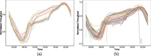
Fig. 6 Test dataset consisting of 63 days of normalized throughput data.

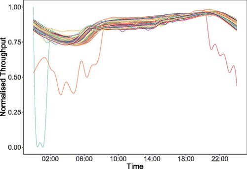
Fig. 7 Figure (a) illustrates the 11 detections returned by FAST, and (b) illustrates the two public holidays on which FAST identifies atypical behavior. In both figures the gray lines represent the days where FAST does not detect anything.

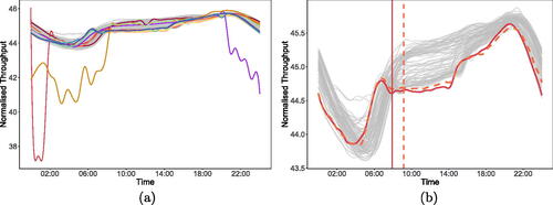
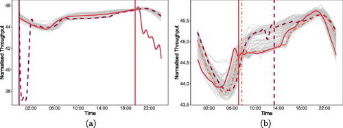
Fig. 8 This figure illustrates a selection of the days on which FAST identifies the emergence of atypical behavior. (a) shows two example magnitude anomalies, while (b) illustrates three example shape anomalies. The vertical lines indicate the point where FAST first identifies this behavior.

To perform FAST, a training dataset (Figure 5(a)) consisting of the first 30 days of the dataset is used. To select the order of the ODE to fit to the training data we use BIC, as described in Section 2.2, and fit an order four ODE to the training data. We then apply FAST to the remaining 89 days with the test threshold set to control the probability of false alarm at the 5% level. 11 alarms are declared, and these instances are depicted in Figure 7(a). One interesting aspect of the results is that two of the days on which a detection takes place are on a public holiday weekend. These are days that are known to have different profiles due to altered consumer behavior, and are shown in Figure 7(b).

FAST detects statistically atypical behavior that reflects both magnitude and shape anomalies in magnitude compared to the profile of the data. We show examples of such instances in Figures 8(a) and (b), respectively. Finally, we remark that the detection delay is less than 40 min from when the atypical behavior appears to start. This illustrates how FAST is able to respond quickly to these events as they emerge in this dataset.

6 Discussion

In this article we have introduced FAST, a new method for detecting the emergence of anomalous structures within functional data. FAST models the underlying profile for the data using PDA and identifies anomalies using a nonparametric CUSUM test. The main advantage of our method is that it is able to detect anomalous profiles as they are received, rather than requiring the complete profile to be observed.

In addition to the methodological contributions made by this work, several theoretical results have been derived for FAST. One of these allows for a user to set a threshold that controls the rate of false alarms observed when no anomaly is present, and simulation studies have shown this to be effective in a finite sample setting.

Simulation studies have also shown the effective performance of FAST for a range of different settings, including those where the assumptions of our model are not satisfied. Furthermore, we have shown how FAST can perform well when the ODE order is over-specified, or when the training data is contaminated with a small number of anomalies. As the contamination increases, however, we see that detection power is reduced, although a practical way to address this would be to first screen the training data with an offline functional anomaly detection method.

To complement our simulations exploring the performance of FAST when detecting emergent anomalies, we have explored how a restriction of FAST can be applied offline in Section 4.5, and Section A in the supplementary material. While the results broadly appear encouraging, and highlight situations where (restricted) FAST is at least comparable with true offline detection test, it is important to consider that there are, by design, some situations where it would be preferable to apply an existing offline detector. For example, in FAST we assume that the non-anomalous observations all follow a similar profile; however, when detecting magnitude anomalies offline not all depth based approaches require this. As another example, the computational complexity of an (offline) FPCA projection is $\mathcal{O}(n^{2}T)$, compared to the $\mathcal{O}(m^3{n}^{2}T)$ cost of using PDA to estimate the differential operator for FAST. While the benefit of using PDA is that the differential operator can be applied to new profiles as they are received for, in an offline setting this is not required as all the data are available upfront and so it may be more efficient to use an FPCA method.

Finally, we return to reflect on the primary motivation for this work: the sequential detection of anomalous structure within functional data. In addition to the encouraging simulation results, we have demonstrated that FAST can detect emerging atypical behaviors in network throughput data.

Supplementary Materials

The supplementary material contains (a) a pdf file with further simulation results repeating the simulations of Sections 4.1, 4.4, and 4.5 but for other underlying profiles, and the proofs of the results in Section 3; and (b) a zip file containing code to reproduce all simulations in the article.

Acknowledgments

The authors would also like to thank Peter Willis (BT), Trevor Burbridge (BT), Steve Cassidy (BT), and James Ramsay for insightful discussions that have helped influence this work. The authors are also grateful to the editorial team and two anonymous referees for their constructive suggestions, and in particular encouraged the inclusion of a comparison with offline methods. Open-source code, making the methods developed in this article accessible, will be made available via an appropriate repository in due course.

Disclosure Statement

The authors report there are no competing interests to declare.

Additional information

Funding

This work was supported by EPSRC grant numbers EP/R004935/1 (NG-CDI) and EP/L015692/1 (STOR-i). Austin also gratefully acknowledges British Telecommunications plc (BT) for providing financial support for his PhD.

References

- Arribas-Gil, A., and Romo, J. (2014), “Shape Outlier Detection and Visualization for Functional Data: The Outliergram,” Biostatistics, 15, 603–619. DOI: 10.1093/biostatistics/kxu006.
- Colosimo, B. M., and Pacella, M. (2010), “A Comparison Study of Control Charts for Statistical Monitoring of Functional Data,” International Journal of Production Research, 48, 1575–1601. DOI: 10.1080/00207540802662888.
- Dai, W., and Genton, M. (2018), “Multivariate Functional Data Visualization and Outlier Detection,” Journal of Computational and Graphical Statistics, 27, 923–934. DOI: 10.1080/10618600.2018.1473781.
- Dai, W., Mrkvička, T., Sun, Y., and Genton, M. G. (2020), “Functional Outlier Detection and Taxonomy by Sequential Transformations,” Computational Statistics & Data Analysis, 149, 106960. DOI: 10.1016/j.csda.2020.106960.
- Eichinger, B., and Kirch, C. (2018), “A MOSUM Procedure for the Estimation of Multiple Random Change Points,” Bernoulli, 24, 526–564. DOI: 10.3150/16-BEJ887.
- Flores, M., Naya, S., Fernández-Casal, R., Zaragoza, S., Raña, P., and Tarrío-Saavedra, J. (2020), “Constructing a Control Chart Using Functional Data,” Mathematics, 8, 58. DOI: 10.3390/math8010058.
- Hall, P., Poskitt, D. S., and Presnell, B. (2001), “A Functional Data–Analytic Approach to Signal Discrimination,” Technometrics, 43, 1–9. DOI: 10.1198/00401700152404273.
- Harris, T., Tucker, J. D., Li, B., and Shand, L. (2020), “Elastic Depths for Detecting Shape Anomalies in Functional Data,” Technometrics, 63, 466–476. DOI: 10.1080/00401706.2020.1811156.
- Huang, H., and Sun, Y. (2019), “A Decomposition of Total Variation Depth for Understanding Functional Outliers,” Technometrics, 61, 445–458. DOI: 10.1080/00401706.2019.1574241.
- Hyndman, R. J., and Shang, H. L. (2010), “Rainbow Plots, Bagplots, and Boxplots for Functional Data,” Journal of Computational and Graphical Statistics, 19, 29–45. DOI: 10.1198/jcgs.2009.08158.
- Jarry, G., Delahaye, D., Nicol, F., and Feron, E. (2020), “Aircraft Atypical Approach Detection Using Functional Principal Component Analysis,” Journal of Air Transport Management, 84, 101787. https://www.sciencedirect.com/science/article/pii/S0969699719303266. DOI: 10.1016/j.jairtraman.2020.101787.
- Jeong, M. K., Lu, J.-C., and Wang, N. (2006), “Wavelet-based SPC Procedure for Complicated Functional Data,” International Journal of Production Research, 44, 729–744. DOI: 10.1080/00207540500222647.
- Johnson, R., and Wichern, D. (1988), Applied Multivariate Statistical Analysis, Prentice-Hall Series in Statistics, Upper Saddle River, NJ; Prentice-Hall.
- Liu, C., Gao, X., and Wang, X. (2022), “Data Adaptive Functional Outlier Detection: Analysis of the Paris Bike Sharing System Sata,” Information Sciences, 602, 13–42. https://www.sciencedirect.com/science/article/pii/S0020025522003711. DOI: 10.1016/j.ins.2022.04.029.
- López-Pintado, S., and Romo, J. (2011), “A Half-region Depth for Functional Data,” Computational Statistics & Data Analysis, 55, 1679–1695. DOI: 10.1016/j.csda.2010.10.024.
- Nagy, S., Gijbels, I., and Hlubinka, D. (2016), “Weak Convergence of Discretely Observed Functional Data with Applications,” Journal of Multivariate Analysis, 146, 46–62. Special Issue on Statistical Models and Methods for High or Infinite Dimensional Spaces. DOI: 10.1016/j.jmva.2015.06.006.
- Ojo, O. T., Lillo, R. E., and Fernandez Anta, A. (2021), fdaoutlier: Outlier Detection Tools for Functional Data Analysis, R package version 0.2.0, available at https://CRAN.R-project.org/package=fdaoutlier.
- Paynabar, K., Zou, C., and Qiu, P. (2016), “A Change-Point Approach for Phase-I Analysis in Multivariate Profile Monitoring and Diagnosis,” Technometrics, 58, 191–204. DOI: 10.1080/00401706.2015.1042168.
- Ramsay, J. (2005), Functional Data Analysis (2nd ed.), Dordrecht: Springer.
- Ramsay, J. (2023), fda: Functional Data Analysis, R package version 6.1.4, available at https://CRAN.R-project.org/package=fda.
- Ramsay, J. O. (1996), “Principal Differential Analysis: Data Reduction by Differential Operators,” Journal of the Royal Statistical Society, Series B, 58, 495–508. DOI: 10.1111/j.2517-6161.1996.tb02096.x.
- Rasmussen, C., and Williams, C. (2005), Gaussian Processes for Machine Learning, Adaptive Computation and Machine Learning Series, Cambridge, MA: MIT Press.
- Rieser, C., and Filzmoser, P. (2022), “Outlier Detection for Pandemic-Related Data Using Compositional Functional Data Analysis,” in Pandemics: Insurance and Social Protection, eds. M. del Carmen Boado-Penas, J. Eisenberg, and Ş. Şahin, pp. 251–266, Cham: Springer.
- Rousseeuw, P. J., Raymaekers, J., and Hubert, M. (2018), “A Measure of Directional Outlyingness With Applications to Image Data and Video,” Journal of Computational and Graphical Statistics, 27, 345–359. DOI: 10.1080/10618600.2017.1366912.
- Schwarz, G. (1978), “Estimating the Dimension of a Model,” The Annals of Statistics, 6, 461–464. DOI: 10.1214/aos/1176344136.
- Staerman, G., Adjakossa, E., Mozharovskyi, P., Hofer, V., Sen Gupta, J., and Clémençon, S. (2023), “Functional Anomaly Detection: A Benchmark Study,” International Journal of Data Science and Analytics, 16, 101–117. DOI: 10.1007/s41060-022-00366-5.
- Talagala, P. D., Hyndman, R. J., Smith-Miles, K., Kandanaarachchi, S., and Muñoz, M. A. (2020), “Anomaly Detection in Streaming Nonstationary Temporal Data,” Journal of Computational and Graphical Statistics, 29, 13–27. DOI: 10.1080/10618600.2019.1617160.
- Tartakovsky, A., Nikiforov, I., and Basseville, M. (2014), Sequential Analysis: Hypothesis Testing and Changepoint Detection, Boca Raton, FL: CRC Press.
- Tartakovsky, A. G., Rozovskii, B. L., and Shah, K. (2005), “A Nonparametric Multichart CUSUM Test for Rapid Intrusion Detection,” in Proceedings of Joint Statistical Meetings (Vol. 7).
- Teräsvirta, T., and Mellin, I. (1986), “Model Selection Criteria and Model Selection Tests in Regression Models,” Scandinavian Journal of Statistics, 13, 159–171.
- Wang, X., Lin, J., Patel, N., and Braun, M. (2018), “Exact Variable-Length Anomaly Detection Algorithm for Univariate and Multivariate Time Series,” Data Mining and Knowledge Discovery, 32, 1806–1844. DOI: 10.1007/s10618-018-0569-7.
- Wolf, H. P. (2019), aplpack: Another Plot Package (version 190512), available at https://cran.r-project.org/package=aplpack.
- Woodall, W. H. (2007), “Current Research on Profile Monitoring,” Production, 17, 420–425. DOI: 10.1590/S0103-65132007000300002.
- Woodall, W. H., Spitzner, D. J., Montgomery, D. C., and Gupta, S. (2004), “Using Control Charts to Monitor Process and Product Quality Profiles,” Journal of Quality Technology, 36, 309–320. DOI: 10.1080/00224065.2004.11980276.
- Yan, H., Paynabar, K., and Shi, J. (2018), “Real-Time Monitoring of High-Dimensional Functional Data Streams via Spatio-Temporal Smooth Sparse Decomposition,” Technometrics, 60, 181–197. DOI: 10.1080/00401706.2017.1346522.
- Zhang, R., Mei, Y., and Shi, J. (2018), “Wavelet-Based Profile Monitoring Using Order-Thresholding Recursive CUSUM Schemes,” in New Frontiers of Biostatistics and Bioinformatics, eds. Y. Zhao and D.-G. Chen, pp. 141–159, Cham: Springer.