Integrated simulation and control environment for the development and safe start-up of cable driven parallel robots

ABSTRACT

This article presents a new environment designed to facilitate the conceptualization and automation of CDPRs (Cable Driven Parallel Robots). Utilizing a platform for robotic simulation, an industrial controller, and a data gateway to communicate both systems, it is possible to emulate CDPR motion in early design, development, and start-up phases. Thus, this simulation environment allows to test how the robot will behave in advance in order to obtain a safer and more reliable first operation with the real robot. An spatially under-constrained CDPR with four cables was used to validate the capabilities of the proposed integrated environment, comparing its performance against an industry-standard hardware prototype. Both the simulation model and the real prototype performed the same trajectory in order to assess a time delay and position errors between them. Evaluation results revealed that the simulation accurately replicated the performance of its industrial counterpart, with a peak divergence of 0.27% in the position of the robot under various speed scenarios. This occurs even when accounting for latency arising from data exchange connecting the industrial control unit to the simulation. The results have shown that the environment is suitable for trajectory control of new CDPR architectures under different dynamic conditions.

Graphical Abstract

KEYWORDS:

• Cable-driven parallel robot
• simulation and real-time control integration
• automation

1. Introduction

Cable-driven parallel robots (CDPRs) are distinguished by the utilization of cables to change the spatial positioning and orientation of their end-effector. Since their introduction in the mid-1980s by Landsberger and Sheridan (Z. Zhang et al. 2022), there has been a sustained trajectory of advancement in CDPR technology. This journey of progress encompasses earlier models like the SkyCam, RoboCrane, and FAST, and extends to more recent systems such as CoGiRo, IPAnema, and FASTKIT (Hussein et al. 2021). In contrast to other parallel manipulators that can manage both tensile and compressive forces on their links, such as Delta robots, CDPRs are inherently constrained to delivering only tensile forces due to their reliance on cables (González-Rodríguez et al. 2023). Nevertheless, the integration of cables into these robots confers multiple comparative advantages over conventional configurations. These benefits include lower inertia, higher payload-to-weight ratio, higher dynamic performance, larger workspace, and higher modularity and reconfigurability (Qian et al. 2018).

Extensive research has been conducted into CDPR architectures, aiming to adapt robots for various applications such as additive manufacturing (Izard et al. 2018), assembly operations (Pan et al. 2020), logistics (Alias et al. 2018), and simulators (Rodriguez-Barroso et al. 2023). Despite the potential advantages of CDPRs across diverse scenarios, their industrial application has been limited. This limitation is primarily due to the lack of commercialized systems and the challenges associated with meeting safety and operational requirements involving standard industry controllers for their implementation.

The effective deployment of these robots could be enhanced by flexible and safe start-up environments. However, such support is not commonly provided by industrial controller manufacturers, particularly for diverse configurations and variants of CDPRs. A few industrial controller manufacturers do offer robotic resources for developing several types of robots, including 2D cartesian, 3D cartesian, gantry, SCARA, and Delta robots. Some of them has distinguished itself by offering built-in modules specifically for developing spatial under-constrained CDPRs with three and four cables (South African Instrumentation and Control 2008). Yet, for unique CDPR configurations, such as those involving an increase or decrease in the number of cables or a new spatial arrangement of the cables, new modelling and development from the ground up would still be necessary. Simulation resources are then needed to support the development and safe evaluation before going to real conditions for the first time. Such resources include, for instance, tools to test kinematics, dynamics, and motion of new robots without the need to build a physical model. Several environments have contributed to cable-robot modelling, analysis, control and simulation, such as WireX (Pott 2019), CASPR (Lau et al. 2016) and CDPR Studio (McDonald, Steven, and Marc 2022). However, none of these tools allows the user to govern the simulation from the industrial controller that will be used in the real prototype, being able to test different control algorithms and path planners. In this article, CoppeliaSim, which is a well-known and versatile robot simulation software, is used as the simulation platform.

This article introduces a tailored environment for the design and automation of CDPRs, such as those featuring standard and non-standard number of cables or distinct motor placements within the robot’s framework. To test the platform’s ability to emulate CDPR motion trajectories in the early stages of the design and/or commissioning of such robots, a spatially under-constrained CDPR of four cables is simulated within the platform.

Obtaining feedback on the position of the robot end-effector is also essential to quantitatively track the spatial trajectory. For the case of CDPR there are different methods, and, in this research, they were implemented in the industrial controller and their performance compared. Subsequently, the performance of the simulated model and the prototype using industry-standard hardware are compared when performing a spatial trajectory. In this way, both systems will be validated and the path to follow for the development of CDPRs will be outlined. The result is a reliable and safe environment to evaluate new configurations and to support the transfer from the laboratory to real conditions of new CDPR configurations.

The article is structured as follows. Section 2 introduces the kinematic modelling of the CDPR used in this research. Section 3 provides a detailed look into the environment used to validate CDPR configurations, considering the simulation software, the use of a standard industrial controller, and the prototype for validation. Section 4 presents the results and discussion of three experiments. These experiments assessed direct kinematics calculation methods, evaluated the reaction time between setpoints in the industrial controller and position feedback of the robot, and analysed trajectory errors in both the simulated model and real prototype. Finally, the article ends with conclusions, limitations, and future work (Section 5).

2. Cable-driven parallel robot modelling

The literature classifies CDPRs according to several criteria, including the working space and the ratio between the number of cables $\mathit{m}$ and the degrees of freedom (DoF) $\mathit{n}$. According to the workspace, CDPRs are classified as either planar or spatial due to their motion in the plane or in space (Zarebidoki, Singh Dhupia, and Xu 2022). 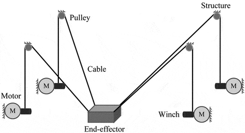According to the relationship between $\mathit{m}$ and $\mathit{n}$, CDPRs are classified as under-constrained (m < n), incompletely constrained (m = n), fully constrained (m = n + 1) and redundantly constrained (m > n + 1) (Z. Zhang et al. 2022). A CDPR is considered under-constrained when it is possible to change its position and orientation without changing the length of its cables. Thus, the robot used in this research was a spatial under-constrained CDPR of four cables and three DoF (Figure 1).

Figure 1. Under-constrained CDPR schematic view.

2.1. Kinematics

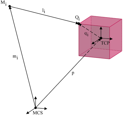
To obtain the kinematic model of the CDPR, the cables are considered to be mass-less and non-elastic. The closed vector loop shown in Figure 2 for a cable $\mathit{i}$ is used to define the kinematic equations of the under-constrained CDPR by four cables of length ($l_i$). In this Figure 2, $m_i$ represents the Cartesian coordinates of the proximal exit points ($M_i)$ to the MCS, $q_i$ denotes the Cartesian coordinates of the distal anchor points ($Q_i)$ to the TCP (Tool Centre Point), and the position and orientation of the TCP is defined by the position vector ($\mathit{p}$) and the rotation matrix ($R_0$) to the MCS, respectively. Thus, the general expression that describes the close-loop vector for the CDPR is:

Figure 2. Closed-loop kinematics model of CDPR.

(1) $m_i+l_i=\mathit{p}+R_0{\mathrm{q}}_{\mathrm{i}}$(1)

2.1.1. Inverse kinematics

The inverse kinematics makes it possible to know the length of each cable from a specific position in space. Given the geometry and the number of cables of this CDPR, it is only possible to control the position of the robot, and not its orientation. Therefore, R becomes the identity matrix. The equation describing the length of the cables $l_i$ can be rewritten from Equation 1(1) $m_i+l_i=\mathit{p}+R_0{\mathrm{q}}_{\mathrm{i}}$(1) as follows:

(2) $l_i=-m_i+q_i+\mathit{p}$(2)

where the position vectors of the distal anchor points $m_i$ and the position vectors of the proximal anchor points $Q_i$ are represented by Equations 3(3) $m_i=\left[\begin{array}{cc}\begin{array}{cc}{m}_1& m_2\end{array}& \begin{array}{cc}{m}_3& m_4\end{array}\end{array}\right]=\left[\begin{array}{cc}\begin{array}{cc}\begin{array}{c}\begin{array}{c}-\frac{B_l}{2}\\ -\frac{B_w}{2}\end{array}\\ B_h\end{array}& \begin{array}{c}\begin{array}{c}\frac{B_l}{2}\\ -\frac{B_w}{2}\end{array}\\ B_h\end{array}\end{array}& \begin{array}{cc}\begin{array}{c}\begin{array}{c}\frac{B_l}{2}\\ \frac{B_w}{2}\end{array}\\ B_h\end{array}& \begin{array}{c}\begin{array}{c}-\frac{B_l}{2}\\ \frac{B_w}{2}\end{array}\\ B_h\end{array}\end{array}\end{array}\right]=\left[\begin{array}{cc}\begin{array}{cc}\begin{array}{c}\begin{array}{c}{m}_{1\mathit{x}}\\ m_{1\mathit{y}}\end{array}\\ m_{1\mathit{z}}\end{array}& \begin{array}{c}\begin{array}{c}{m}_{2\mathit{x}}\\ m_{2\mathit{y}}\end{array}\\ m_{2\mathit{z}}\end{array}\end{array}& \begin{array}{cc}\begin{array}{c}\begin{array}{c}{m}_{3\mathit{x}}\\ m_{3\mathit{y}}\end{array}\\ m_{3\mathit{z}}\end{array}& \begin{array}{c}\begin{array}{c}{m}_{4\mathit{x}}\\ m_{4\mathit{y}}\end{array}\\ m_{4\mathit{z}}\end{array}\end{array}\end{array}\right]$(3) and 4(4) $q_i=\left[\begin{array}{cc}\begin{array}{cc}{q}_1& q_2\end{array}& \begin{array}{cc}{q}_3& q_4\end{array}\end{array}\right]=\left[\begin{array}{cc}\begin{array}{cc}\begin{array}{c}\begin{array}{c}-\frac{T_l}{2}\\ -\frac{T_w}{2}\end{array}\\ \frac{T_h}{2}\end{array}& \begin{array}{c}\begin{array}{c}\frac{T_l}{2}\\ -\frac{T_w}{2}\end{array}\\ \frac{T_h}{2}\end{array}\end{array}& \begin{array}{cc}\begin{array}{c}\begin{array}{c}\frac{T_l}{2}\\ \frac{T_w}{2}\end{array}\\ \frac{T_h}{2}\end{array}& \begin{array}{c}\begin{array}{c}-\frac{T_l}{2}\\ \frac{T_w}{2}\end{array}\\ \frac{T_h}{2}\end{array}\end{array}\end{array}\right]=\left[\begin{array}{cc}\begin{array}{cc}\begin{array}{c}\begin{array}{c}{q}_{1\mathit{x}}\\ q_{1\mathit{y}}\end{array}\\ q_{1\mathit{z}}\end{array}& \begin{array}{c}\begin{array}{c}{q}_{2\mathit{x}}\\ q_{2\mathit{y}}\end{array}\\ q_{2\mathit{z}}\end{array}\end{array}& \begin{array}{cc}\begin{array}{c}\begin{array}{c}{q}_{3\mathit{x}}\\ q_{3\mathit{y}}\end{array}\\ q_{3\mathit{z}}\end{array}& \begin{array}{c}\begin{array}{c}{q}_{4\mathit{x}}\\ q_{4\mathit{y}}\end{array}\\ q_{4\mathit{z}}\end{array}\end{array}\end{array}\right]$(4) :

(3) $m_i=\left[\begin{array}{cc}\begin{array}{cc}{m}_1& m_2\end{array}& \begin{array}{cc}{m}_3& m_4\end{array}\end{array}\right]=\left[\begin{array}{cc}\begin{array}{cc}\begin{array}{c}\begin{array}{c}-\frac{B_l}{2}\\ -\frac{B_w}{2}\end{array}\\ B_h\end{array}& \begin{array}{c}\begin{array}{c}\frac{B_l}{2}\\ -\frac{B_w}{2}\end{array}\\ B_h\end{array}\end{array}& \begin{array}{cc}\begin{array}{c}\begin{array}{c}\frac{B_l}{2}\\ \frac{B_w}{2}\end{array}\\ B_h\end{array}& \begin{array}{c}\begin{array}{c}-\frac{B_l}{2}\\ \frac{B_w}{2}\end{array}\\ B_h\end{array}\end{array}\end{array}\right]=\left[\begin{array}{cc}\begin{array}{cc}\begin{array}{c}\begin{array}{c}{m}_{1\mathit{x}}\\ m_{1\mathit{y}}\end{array}\\ m_{1\mathit{z}}\end{array}& \begin{array}{c}\begin{array}{c}{m}_{2\mathit{x}}\\ m_{2\mathit{y}}\end{array}\\ m_{2\mathit{z}}\end{array}\end{array}& \begin{array}{cc}\begin{array}{c}\begin{array}{c}{m}_{3\mathit{x}}\\ m_{3\mathit{y}}\end{array}\\ m_{3\mathit{z}}\end{array}& \begin{array}{c}\begin{array}{c}{m}_{4\mathit{x}}\\ m_{4\mathit{y}}\end{array}\\ m_{4\mathit{z}}\end{array}\end{array}\end{array}\right]$(3)

(4) $q_i=\left[\begin{array}{cc}\begin{array}{cc}{q}_1& q_2\end{array}& \begin{array}{cc}{q}_3& q_4\end{array}\end{array}\right]=\left[\begin{array}{cc}\begin{array}{cc}\begin{array}{c}\begin{array}{c}-\frac{T_l}{2}\\ -\frac{T_w}{2}\end{array}\\ \frac{T_h}{2}\end{array}& \begin{array}{c}\begin{array}{c}\frac{T_l}{2}\\ -\frac{T_w}{2}\end{array}\\ \frac{T_h}{2}\end{array}\end{array}& \begin{array}{cc}\begin{array}{c}\begin{array}{c}\frac{T_l}{2}\\ \frac{T_w}{2}\end{array}\\ \frac{T_h}{2}\end{array}& \begin{array}{c}\begin{array}{c}-\frac{T_l}{2}\\ \frac{T_w}{2}\end{array}\\ \frac{T_h}{2}\end{array}\end{array}\end{array}\right]=\left[\begin{array}{cc}\begin{array}{cc}\begin{array}{c}\begin{array}{c}{q}_{1\mathit{x}}\\ q_{1\mathit{y}}\end{array}\\ q_{1\mathit{z}}\end{array}& \begin{array}{c}\begin{array}{c}{q}_{2\mathit{x}}\\ q_{2\mathit{y}}\end{array}\\ q_{2\mathit{z}}\end{array}\end{array}& \begin{array}{cc}\begin{array}{c}\begin{array}{c}{q}_{3\mathit{x}}\\ q_{3\mathit{y}}\end{array}\\ q_{3\mathit{z}}\end{array}& \begin{array}{c}\begin{array}{c}{q}_{4\mathit{x}}\\ q_{4\mathit{y}}\end{array}\\ q_{4\mathit{z}}\end{array}\end{array}\end{array}\right]$(4)

where $B_l$, $B_w$ and $B_h$ are the length, width, and height of the base, and $T_l$, $T_w$ and $T_h$ length, width and, height of the tool. Table 1 shows the geometrical parameters of the CDPR used in this research. A tool height of zero was determined as it was considered to locate the reference for the movement on the top face of the tool.

Table 1. Geometrical parameters of the CDPR.

Parameter	$B_l$	$B_w$	$B_h$	$T_l$	$T_w$	$T_h$
Value [mm]	890	1520	1450	58	103	0

Finally, substituting Equation 3(3) $m_i=\left[\begin{array}{cc}\begin{array}{cc}{m}_1& m_2\end{array}& \begin{array}{cc}{m}_3& m_4\end{array}\end{array}\right]=\left[\begin{array}{cc}\begin{array}{cc}\begin{array}{c}\begin{array}{c}-\frac{B_l}{2}\\ -\frac{B_w}{2}\end{array}\\ B_h\end{array}& \begin{array}{c}\begin{array}{c}\frac{B_l}{2}\\ -\frac{B_w}{2}\end{array}\\ B_h\end{array}\end{array}& \begin{array}{cc}\begin{array}{c}\begin{array}{c}\frac{B_l}{2}\\ \frac{B_w}{2}\end{array}\\ B_h\end{array}& \begin{array}{c}\begin{array}{c}-\frac{B_l}{2}\\ \frac{B_w}{2}\end{array}\\ B_h\end{array}\end{array}\end{array}\right]=\left[\begin{array}{cc}\begin{array}{cc}\begin{array}{c}\begin{array}{c}{m}_{1\mathit{x}}\\ m_{1\mathit{y}}\end{array}\\ m_{1\mathit{z}}\end{array}& \begin{array}{c}\begin{array}{c}{m}_{2\mathit{x}}\\ m_{2\mathit{y}}\end{array}\\ m_{2\mathit{z}}\end{array}\end{array}& \begin{array}{cc}\begin{array}{c}\begin{array}{c}{m}_{3\mathit{x}}\\ m_{3\mathit{y}}\end{array}\\ m_{3\mathit{z}}\end{array}& \begin{array}{c}\begin{array}{c}{m}_{4\mathit{x}}\\ m_{4\mathit{y}}\end{array}\\ m_{4\mathit{z}}\end{array}\end{array}\end{array}\right]$(3) and Equation 4(4) $q_i=\left[\begin{array}{cc}\begin{array}{cc}{q}_1& q_2\end{array}& \begin{array}{cc}{q}_3& q_4\end{array}\end{array}\right]=\left[\begin{array}{cc}\begin{array}{cc}\begin{array}{c}\begin{array}{c}-\frac{T_l}{2}\\ -\frac{T_w}{2}\end{array}\\ \frac{T_h}{2}\end{array}& \begin{array}{c}\begin{array}{c}\frac{T_l}{2}\\ -\frac{T_w}{2}\end{array}\\ \frac{T_h}{2}\end{array}\end{array}& \begin{array}{cc}\begin{array}{c}\begin{array}{c}\frac{T_l}{2}\\ \frac{T_w}{2}\end{array}\\ \frac{T_h}{2}\end{array}& \begin{array}{c}\begin{array}{c}-\frac{T_l}{2}\\ \frac{T_w}{2}\end{array}\\ \frac{T_h}{2}\end{array}\end{array}\end{array}\right]=\left[\begin{array}{cc}\begin{array}{cc}\begin{array}{c}\begin{array}{c}{q}_{1\mathit{x}}\\ q_{1\mathit{y}}\end{array}\\ q_{1\mathit{z}}\end{array}& \begin{array}{c}\begin{array}{c}{q}_{2\mathit{x}}\\ q_{2\mathit{y}}\end{array}\\ q_{2\mathit{z}}\end{array}\end{array}& \begin{array}{cc}\begin{array}{c}\begin{array}{c}{q}_{3\mathit{x}}\\ q_{3\mathit{y}}\end{array}\\ q_{3\mathit{z}}\end{array}& \begin{array}{c}\begin{array}{c}{q}_{4\mathit{x}}\\ q_{4\mathit{y}}\end{array}\\ q_{4\mathit{z}}\end{array}\end{array}\end{array}\right]$(4) into Equation 2(2) $l_i=-m_i+q_i+\mathit{p}$(2) , the solution for the inverse kinematics for each cable is obtained (Equation 5(5) $\left\{\begin{array}{c}{l}_1=\sqrt{{\left(-\frac{T_l}{2}+\frac{B_l}{2}+\mathit{x}\right)}^2+{\left(-\frac{T_w}{2}+\frac{B_w}{2}+\mathit{y}\right)}^2+{\left(\frac{T_h}{2}-B_h+\mathit{z}\right)}^2}\\ l_2=\sqrt{{\left(\frac{T_l}{2}-\frac{B_l}{2}+\mathit{x}\right)}^2+{\left(-\frac{T_w}{2}+\frac{B_w}{2}+\mathit{y}\right)}^2+{\left(\frac{T_h}{2}-B_h+\mathit{z}\right)}^2}\\ l_3=\sqrt{{\left(\frac{T_l}{2}-\frac{B_l}{2}+\mathit{x}\right)}^2+{\left(\frac{T_w}{2}-\frac{B_w}{2}+\mathit{y}\right)}^2+{\left(\frac{T_h}{2}-B_h+\mathit{z}\right)}^2}\\ l_4=\sqrt{{\left(-\frac{T_l}{2}+\frac{B_l}{2}+\mathit{x}\right)}^2+{\left(\frac{T_w}{2}-\frac{B_w}{2}+\mathit{y}\right)}^2+{\left(\frac{T_h}{2}-B_h+\mathit{z}\right)}^2}\end{array}\right.$(5) ).

(5) $\left\{\begin{array}{c}{l}_1=\sqrt{{\left(-\frac{T_l}{2}+\frac{B_l}{2}+\mathit{x}\right)}^2+{\left(-\frac{T_w}{2}+\frac{B_w}{2}+\mathit{y}\right)}^2+{\left(\frac{T_h}{2}-B_h+\mathit{z}\right)}^2}\\ l_2=\sqrt{{\left(\frac{T_l}{2}-\frac{B_l}{2}+\mathit{x}\right)}^2+{\left(-\frac{T_w}{2}+\frac{B_w}{2}+\mathit{y}\right)}^2+{\left(\frac{T_h}{2}-B_h+\mathit{z}\right)}^2}\\ l_3=\sqrt{{\left(\frac{T_l}{2}-\frac{B_l}{2}+\mathit{x}\right)}^2+{\left(\frac{T_w}{2}-\frac{B_w}{2}+\mathit{y}\right)}^2+{\left(\frac{T_h}{2}-B_h+\mathit{z}\right)}^2}\\ l_4=\sqrt{{\left(-\frac{T_l}{2}+\frac{B_l}{2}+\mathit{x}\right)}^2+{\left(\frac{T_w}{2}-\frac{B_w}{2}+\mathit{y}\right)}^2+{\left(\frac{T_h}{2}-B_h+\mathit{z}\right)}^2}\end{array}\right.$(5)

2.1.2. Direct kinematics

Direct kinematics focuses on determining the end-effector’s position and orientation using the length values of each cable. A geometric method can be used in some cases to obtain a closed solution. Specifically, when there are three base points connected to a platform connection point, the task involves finding the intersection points of three spheres, provided that the unstrained length of the cable is greater than the Euclidean distance between the exit point and the mobile platform (Chawla et al. 2023). The main advantage of using a geometric method is that it is faster and more accurate than numerical methods. Nonetheless, analytical solutions are engaged with highly coupled nonlinear equations that are difficult to solve analytically to obtain exact answers, requiring the use of numerical methods to find a solution in most cases (Kalajahi, Mahboubkhah, and Barari 2021). The numerical methods approach can be computationally demanding, particularly when real-time computation is required but is good enough to obtain an approximate solution independently of the specific geometry relations between cables of the CDPR. Both methods are detailed below and their implementation was used to perform the experimental evaluation in section 4.

2.1.2.1. Analytical method

The analytical method focuses on the closed-form solution of the inverse kinematics. Rearranging the equation 5(5) $\left\{\begin{array}{c}{l}_1=\sqrt{{\left(-\frac{T_l}{2}+\frac{B_l}{2}+\mathit{x}\right)}^2+{\left(-\frac{T_w}{2}+\frac{B_w}{2}+\mathit{y}\right)}^2+{\left(\frac{T_h}{2}-B_h+\mathit{z}\right)}^2}\\ l_2=\sqrt{{\left(\frac{T_l}{2}-\frac{B_l}{2}+\mathit{x}\right)}^2+{\left(-\frac{T_w}{2}+\frac{B_w}{2}+\mathit{y}\right)}^2+{\left(\frac{T_h}{2}-B_h+\mathit{z}\right)}^2}\\ l_3=\sqrt{{\left(\frac{T_l}{2}-\frac{B_l}{2}+\mathit{x}\right)}^2+{\left(\frac{T_w}{2}-\frac{B_w}{2}+\mathit{y}\right)}^2+{\left(\frac{T_h}{2}-B_h+\mathit{z}\right)}^2}\\ l_4=\sqrt{{\left(-\frac{T_l}{2}+\frac{B_l}{2}+\mathit{x}\right)}^2+{\left(\frac{T_w}{2}-\frac{B_w}{2}+\mathit{y}\right)}^2+{\left(\frac{T_h}{2}-B_h+\mathit{z}\right)}^2}\end{array}\right.$(5) for the first cable length, Equation 6(6) $l_1^2=\mathit{\hspace{0.17em}}{\left(\mathit{x}+\left({\mathit{q}}_{1\mathit{x}}-m_{1\mathit{x}}\right)\right)}^2+{\left(\mathit{y}+\left({\mathit{q}}_{1\mathit{y}}-m_{1\mathit{y}}\mathit{\hspace{0.17em}}\right)\right)}^2+{\left(\mathit{z}+\left({\mathit{q}}_{1\mathit{z}}-m_{1\mathit{z}}\right)\right)}^2$(6) is given:

(6) $l_1^2=\mathit{\hspace{0.17em}}{\left(\mathit{x}+\left({\mathit{q}}_{1\mathit{x}}-m_{1\mathit{x}}\right)\right)}^2+{\left(\mathit{y}+\left({\mathit{q}}_{1\mathit{y}}-m_{1\mathit{y}}\mathit{\hspace{0.17em}}\right)\right)}^2+{\left(\mathit{z}+\left({\mathit{q}}_{1\mathit{z}}-m_{1\mathit{z}}\right)\right)}^2$(6)

Equation 6(6) $l_1^2=\mathit{\hspace{0.17em}}{\left(\mathit{x}+\left({\mathit{q}}_{1\mathit{x}}-m_{1\mathit{x}}\right)\right)}^2+{\left(\mathit{y}+\left({\mathit{q}}_{1\mathit{y}}-m_{1\mathit{y}}\mathit{\hspace{0.17em}}\right)\right)}^2+{\left(\mathit{z}+\left({\mathit{q}}_{1\mathit{z}}-m_{1\mathit{z}}\right)\right)}^2$(6) represents a sphere with the cable length as the radius and the difference between base points and the tool points as the coordinates of the centre of the sphere. Since the robot has four cables, there are a total of four spheres. Considering that the CDPR has three degrees of freedom, it requires three cable length values to determine the position of the end-effector. The aim, then, is to find the equation of the line (Equation 7(7) $\mathrm{s}\left(\mathrm{x},\mathrm{y},\mathrm{z}\right)={\mathrm{p}}_0\left(\mathrm{x},\mathrm{y},\mathrm{z}\right)+\mathrm{v}\left(\mathrm{x},\mathrm{y},\mathrm{z}\right)\mathrm{t}$(7) ) that intersects the three spheres, thereby obtaining the two solution points:

(7) $\mathrm{s}\left(\mathrm{x},\mathrm{y},\mathrm{z}\right)={\mathrm{p}}_0\left(\mathrm{x},\mathrm{y},\mathrm{z}\right)+\mathrm{v}\left(\mathrm{x},\mathrm{y},\mathrm{z}\right)\mathrm{t}$(7)

where, $\mathit{s}$ represents the equation of the line, $p_0$ is a point on the line, $\mathit{v}$ is the direction vector and $\mathit{t}$ is the variable of the line in parametric form. Thus, the process is as follows (Mersi et al. 2018) and was adapted to be run on an industrial controller:

1. The three sphere equations are obtained. For this method the equation of the sphere is needed as shown in Equation 8.(8) ${\mathrm{x}}^2+y^2+z^2+A_1\mathit{x}+B_1\mathit{x}+C_1\mathit{z}+D_1=0$(8) Rearranging Equation 6(6) $l_1^2=\mathit{\hspace{0.17em}}{\left(\mathit{x}+\left({\mathit{q}}_{1\mathit{x}}-m_{1\mathit{x}}\right)\right)}^2+{\left(\mathit{y}+\left({\mathit{q}}_{1\mathit{y}}-m_{1\mathit{y}}\mathit{\hspace{0.17em}}\right)\right)}^2+{\left(\mathit{z}+\left({\mathit{q}}_{1\mathit{z}}-m_{1\mathit{z}}\right)\right)}^2$(6) and considering Equation 8(8) ${\mathrm{x}}^2+y^2+z^2+A_1\mathit{x}+B_1\mathit{x}+C_1\mathit{z}+D_1=0$(8) , Equation 9(9) $\left\{\begin{array}{c}{\mathrm{A}}_1=2{\mathrm{q}}_{\mathrm{x}1}-2m_{\mathit{x}1}\\ {\mathrm{B}}_1=2{\mathrm{q}}_{\mathrm{y}1}-2m_{\mathit{y}1}\\ {\mathrm{C}}_1=2{\mathrm{q}}_{\mathrm{z}1}-2m_{\mathit{z}1}\\ {\mathrm{D}}_1=A^2+B^2+C^2-l_1^2\end{array}\right.$(9) shows the values of the parameters of the sphere corresponding to the first cable.

   (8) ${\mathrm{x}}^2+y^2+z^2+A_1\mathit{x}+B_1\mathit{x}+C_1\mathit{z}+D_1=0$(8)
   (9) $\left\{\begin{array}{c}{\mathrm{A}}_1=2{\mathrm{q}}_{\mathrm{x}1}-2m_{\mathit{x}1}\\ {\mathrm{B}}_1=2{\mathrm{q}}_{\mathrm{y}1}-2m_{\mathit{y}1}\\ {\mathrm{C}}_1=2{\mathrm{q}}_{\mathrm{z}1}-2m_{\mathit{z}1}\\ {\mathrm{D}}_1=A^2+B^2+C^2-l_1^2\end{array}\right.$(9)

2. Two intersection planes (Equation 10(10) $\left\{\begin{array}{c}{\mathrm{E}}_1\mathit{x}+F_1\mathit{y}+G_1\mathit{z}+H_1=0\\ {\mathrm{E}}_2\mathit{x}+F_2\mathit{y}+G_2\mathit{z}+H_2=0\end{array}\right.$(10) ) between one of the spheres with the other two are obtained. Equation 11(11) $\left\{\begin{array}{c}{\mathrm{E}}_1={\mathrm{A}}_1-A_2\\ {\mathrm{F}}_1={\mathrm{B}}_1-B_2\\ {\mathrm{G}}_1={\mathrm{C}}_1-C_2\\ {\mathrm{H}}_1=D_1-D_2\end{array}\right.$(11) shows the values of the first plane calculated considering the spheres calculated in the previous step (Equation 9(9) $\left\{\begin{array}{c}{\mathrm{A}}_1=2{\mathrm{q}}_{\mathrm{x}1}-2m_{\mathit{x}1}\\ {\mathrm{B}}_1=2{\mathrm{q}}_{\mathrm{y}1}-2m_{\mathit{y}1}\\ {\mathrm{C}}_1=2{\mathrm{q}}_{\mathrm{z}1}-2m_{\mathit{z}1}\\ {\mathrm{D}}_1=A^2+B^2+C^2-l_1^2\end{array}\right.$(9) ).

   (10) $\left\{\begin{array}{c}{\mathrm{E}}_1\mathit{x}+F_1\mathit{y}+G_1\mathit{z}+H_1=0\\ {\mathrm{E}}_2\mathit{x}+F_2\mathit{y}+G_2\mathit{z}+H_2=0\end{array}\right.$(10)
   (11) $\left\{\begin{array}{c}{\mathrm{E}}_1={\mathrm{A}}_1-A_2\\ {\mathrm{F}}_1={\mathrm{B}}_1-B_2\\ {\mathrm{G}}_1={\mathrm{C}}_1-C_2\\ {\mathrm{H}}_1=D_1-D_2\end{array}\right.$(11)

3. This step focuses on obtaining the point $p_0$ (x,y,z) that is contained in the intersection of the two planes. This is achieved by substituting the point in both planes and solving the resulting system of equations (Equation 12(12) $\left\{\begin{array}{c}{\mathrm{E}}_1{p}_{0\mathit{x}}+F_1{p}_{0\mathit{y}}+G_1{p}_{0\mathit{z}}=-H_1\\ {\mathrm{E}}_2{p}_{0\mathit{x}}+F_2{p}_{0\mathit{y}}+G_2{p}_{0\mathit{z}}=-H_2\end{array}\right.$(12) ). For this purpose, one of the spatial values of $p_0$is fixed, i.e. the z-value.

   (12) $\left\{\begin{array}{c}{\mathrm{E}}_1{p}_{0\mathit{x}}+F_1{p}_{0\mathit{y}}+G_1{p}_{0\mathit{z}}=-H_1\\ {\mathrm{E}}_2{p}_{0\mathit{x}}+F_2{p}_{0\mathit{y}}+G_2{p}_{0\mathit{z}}=-H_2\end{array}\right.$(12)

4. Applying the cross product between the normal vectors ($n_1$ and $n_2$) of each intersection plane is possible to obtain the vector $\mathit{v}$ that is parallel to the line of intersection of both planes (Equation 13(13) $\mathrm{v}=\left[v_x{v}_y{v}_z\right]=n_1\times n_2=\left[E_1{F}_1{G}_1\right]\times \left[E_2{F}_2{G}_2\right]$(13) ).

(13) $\mathrm{v}=\left[v_x{v}_y{v}_z\right]=n_1\times n_2=\left[E_1{F}_1{G}_1\right]\times \left[E_2{F}_2{G}_2\right]$(13)

(5) Considering the mutual point and the parallel vector, it only remains to find the value of $\mathit{t}$ in the equation of the intersection line of both planes. Therefore, by intersecting this line (Equation 7(7) $\mathrm{s}\left(\mathrm{x},\mathrm{y},\mathrm{z}\right)={\mathrm{p}}_0\left(\mathrm{x},\mathrm{y},\mathrm{z}\right)+\mathrm{v}\left(\mathrm{x},\mathrm{y},\mathrm{z}\right)\mathrm{t}$(7) ) with one of the spheres (Equation 6(6) $l_1^2=\mathit{\hspace{0.17em}}{\left(\mathit{x}+\left({\mathit{q}}_{1\mathit{x}}-m_{1\mathit{x}}\right)\right)}^2+{\left(\mathit{y}+\left({\mathit{q}}_{1\mathit{y}}-m_{1\mathit{y}}\mathit{\hspace{0.17em}}\right)\right)}^2+{\left(\mathit{z}+\left({\mathit{q}}_{1\mathit{z}}-m_{1\mathit{z}}\right)\right)}^2$(6) ), the following second-degree equation is obtained (Equation 14(14) ${\left({\mathit{p}}_{0\mathit{x}}+v_x\mathit{\hspace{0.17em}}\mathit{t}-\left(q_{1\mathit{x}}-m_{1\mathit{x}}\right)\right)}^2+{\left({\mathit{p}}_{0\mathit{y}}+v_y\mathit{\hspace{0.17em}}\mathit{t}-\left(q_{1\mathrm{y}}-m_{1\mathrm{y}}\right)\right)}^2+{\left({\mathit{p}}_{0\mathit{z}}+v_z\mathit{\hspace{0.17em}}\mathit{t}-\left(q_{1\mathrm{z}}-m_{1\mathrm{z}}\right)\right)}^2-r^2=0$(14) ).

(14) ${\left({\mathit{p}}_{0\mathit{x}}+v_x\mathit{\hspace{0.17em}}\mathit{t}-\left(q_{1\mathit{x}}-m_{1\mathit{x}}\right)\right)}^2+{\left({\mathit{p}}_{0\mathit{y}}+v_y\mathit{\hspace{0.17em}}\mathit{t}-\left(q_{1\mathrm{y}}-m_{1\mathrm{y}}\right)\right)}^2+{\left({\mathit{p}}_{0\mathit{z}}+v_z\mathit{\hspace{0.17em}}\mathit{t}-\left(q_{1\mathrm{z}}-m_{1\mathrm{z}}\right)\right)}^2-r^2=0$(14)

The solution of Equation 14(14) ${\left({\mathit{p}}_{0\mathit{x}}+v_x\mathit{\hspace{0.17em}}\mathit{t}-\left(q_{1\mathit{x}}-m_{1\mathit{x}}\right)\right)}^2+{\left({\mathit{p}}_{0\mathit{y}}+v_y\mathit{\hspace{0.17em}}\mathit{t}-\left(q_{1\mathrm{y}}-m_{1\mathrm{y}}\right)\right)}^2+{\left({\mathit{p}}_{0\mathit{z}}+v_z\mathit{\hspace{0.17em}}\mathit{t}-\left(q_{1\mathrm{z}}-m_{1\mathrm{z}}\right)\right)}^2-r^2=0$(14) results in the two possible direct kinematics points. However, only one is valid because the other is physically not reachable because it is a solution above the base of the robot.

2.1.2.2. Numerical method

As mentioned above, when the solution of the direct kinematic is not feasible using geometric methods, it is common to use numerical methods to achieve a point very close to the real solution. The direct kinematics of the under-constrained CDPR by four cables is formulated as an optimization problem, which is addressed using the Newton-Raphson iterative numerical analysis method (Song et al. 2023). The objective of the optimization problem is to minimize the difference between the cable lengths calculated by numerical analysis and the actual cable lengths until a convergence value is reached. This requires a closed-form solution that includes four concurrent non-linear equations with four unknown variables which are difficult to solve explicitly. Consequently, the minimization function is as Equation 15:

(15) $\mathit{f}\left(\mathit{a}\right)={\widehat{l_i}}^2-{l_i}^2$(15)

In which (a) represents the minimization function, $\mathit{\alpha }$ is the position vector of the end-effector (EE), $\widehat{l_i}$ denotes the calculated cable lengths, and $l_i\mathit{\hspace{0.17em}}$ refers to the current measured cable lengths. The Newton-Raphson method, when applied to this scenario, yields the subsequent expression (Equation 16(16) ${\left[\begin{array}{c}\mathit{x}\\ \mathit{y}\\ \mathit{z}\end{array}\right]}_{\mathit{n}+1}={\left[\begin{array}{c}\mathit{x}\\ \mathit{y}\\ \mathit{z}\end{array}\right]}_n-{\left[\begin{array}{ccc}\frac{\mathrm{\partial }{f}_1}{\mathrm{\partial x}}& \frac{\mathrm{\partial }{f}_1}{\mathrm{\partial y}}& \frac{\delta f_1}{\mathit{\delta z}}\\ \frac{\mathrm{\partial }{f}_2}{\mathrm{\partial x}}& \frac{\mathrm{\partial }{f}_2}{\mathrm{\partial y}}& \frac{\delta f_2}{\mathit{\delta z}}\\ \frac{\mathrm{\partial }{f}_3}{\mathrm{\partial x}}& \frac{\mathrm{\partial }{f}_3}{\mathrm{\partial }\mathit{y}}& \frac{\delta f_3}{\mathit{\delta z}}\end{array}\right]}_{\mathit{n}}^{-1}{\left[\begin{array}{c}{f}_1\\ f_2\\ f_3\end{array}\right]}_{\mathit{n}}$(16) ). Accordingly, the multiplication between the inverse Jacobian and the function represents the Newton-Raphson convergence factor.

(16) ${\left[\begin{array}{c}\mathit{x}\\ \mathit{y}\\ \mathit{z}\end{array}\right]}_{\mathit{n}+1}={\left[\begin{array}{c}\mathit{x}\\ \mathit{y}\\ \mathit{z}\end{array}\right]}_n-{\left[\begin{array}{ccc}\frac{\mathrm{\partial }{f}_1}{\mathrm{\partial x}}& \frac{\mathrm{\partial }{f}_1}{\mathrm{\partial y}}& \frac{\delta f_1}{\mathit{\delta z}}\\ \frac{\mathrm{\partial }{f}_2}{\mathrm{\partial x}}& \frac{\mathrm{\partial }{f}_2}{\mathrm{\partial y}}& \frac{\delta f_2}{\mathit{\delta z}}\\ \frac{\mathrm{\partial }{f}_3}{\mathrm{\partial x}}& \frac{\mathrm{\partial }{f}_3}{\mathrm{\partial }\mathit{y}}& \frac{\delta f_3}{\mathit{\delta z}}\end{array}\right]}_{\mathit{n}}^{-1}{\left[\begin{array}{c}{f}_1\\ f_2\\ f_3\end{array}\right]}_{\mathit{n}}$(16)

Therefore, if the convergence factor falls below a given threshold, the solution of the new point is considered valid as a solution of the direct kinematics. If the newly calculated point does not meet the convergence criteria, it is then considered as the present point. The process continues by recalculating a new point based on this updated position, iterating until the convergence requirement is satisfied. By using these methods, the position of the CDPR can be known, thus ensuring that it remains within certain movement margins.

3. Architecture of the integrated simulation and control environment

During the design, testing phase, and the first start-up of this type of robot, it is important to understand how the robot can react to certain sequences of movements such as abrupt movement changes, or rapid control strategies to perform these movements in a safe and reliable way. For this reason, having a simulation environment that considers changing dynamics and disturbances is beneficial for the development and commissioning of these robots (Phanden, Sharma, and Dubey 2021).

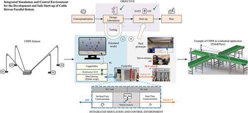
Figure 3 shows the architecture of the proposal which consists of three main components: the robot, which is simulated in CoppeliaSim and built as a physical prototype, the control (industrial controller), and a data gateway (python script) between the simulated robot and the control part.

Figure 3. Architecture of the proposed environment.

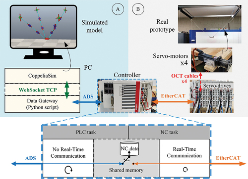
Figure 3 also highlights two alternative use scenarios (A and B) representing the cases of working with the simulated model or with the real robot prototype, respectively. Path A shows the robotic simulator (CoppeliaSim) exchanging data with the industrial controller to perform the movement of the simulated model. This configuration makes it possible to test the algorithm and code implemented directly in the actual industrial controller, but without needing to have the real robot (drives and mechanics), since they are simulated in CoppeliaSim. Alternatively, Path B allows switching from the simulated model (drivers and mechanics) to work with the real counterpart hardware elements (I/O cards, communication protocol, servo-drives, motors, and moving mechanical elements).

3.1. Simulation platform

The simulation model of the CDPR was developed in CoppeliaSim (Robotics 2023c). CoppeliaSim is a robotic simulation platform that allows accurate and fast robot simulations (Pessoa De Melo et al. 2019). It distinguishes itself from other robot simulation tools like Mujoco and Gazebo through its versatility, integrated development environment, support for multiple physics engines, and integration with the Robot Operating System (ROS) (Collins et al. 2021). The use of the CoppeliaSim environment for simulating robotic dynamics adds an additional layer of realism to the simulator. This is crucial for later stages of development, where more complex strategies could be safely and efficiently implemented and tested.

This platform also allows the user to control the behaviour of each model object through scripts from inside the simulator or externally from an application programming interface (API) (T. Zhang et al. 2023). The use of an API facilitates data exchange between the simulator and any other external application or service. Due to the complex nature of physics simulation (accuracy, realism, speed, etc.), CoppeliaSim offers a variety of physics engines (Robotics 2023a). Bullet physics library, which is an open-source physics engine featuring rigid-soft body dynamics, was the one employed in this work.

Regarding simulation within the environment, CoppeliaSim contains two different time steps: a simulation loop timestep and a physics engine loop timestep. The former means that all scripts must run in every simulation cycle. That is, the execution time cannot be longer than the simulation one. By default, the simulation loop timestep is set to 50 ms, although it could be smaller. The physics engine loop timestep entails the physical calculations and it is set to be 10 times faster than the simulation loop time, that is, 5 ms. However, it is recommended to speed up the physics engine to 1 ms-2 ms if a fine-grained dynamic simulation is required. In this research, the simulation loop time was set at 20 ms and the physics engine loop time at 2 ms. The computer used to run CoppeliaSim for this research was a WF65-10TJ laptop equipped with an Intel Core i7-1050 H processor operating at 2.60 GHz and 32GB of DDR4 RAM memory.

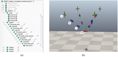
To model the CDPR in the CoppeliaSim platform, a sequence of rigid bodies and joints was used without considering the pulleys-winch system and the cable sagging. Figure 4 shows the tree of components of the robot in CoppeliaSim. Dummy objects are a simple point in the 3D space, and they were used to create the kinematic chains. The pulleys were modelled using rotational passive joints and rigid bodies (A in Figure 4b). The cables were modelled as a sequence of prismatic joints and rigid bodies, since a joint itself is not a physical object that can be connected to another joint directly. The first prismatic joint was responsible for adjusting the length of the cable (B in Figure 4b), The second prismatic joint aimed to mitigate compressive stress on the end-effector (C in Figure 4b), as mentioned in (Zake et al. 2019). To secure the cable’s end to the end-effector, a mechanism like the pulley was utilized (D in Figure 4b).

Figure 4. Under-constrained CDPR model in CoppeliaSim. a) tree of components. (b) 3D view.

Regarding the dynamic properties of the active prismatic joints, the following configuration is highlighted:

• The motor was configured as position-controlled, and the motion was computer-based (CB), allowing it to receive setpoint commands from outside CoppeliaSim.

• The maximum velocity, acceleration, and jerk are limited to 3 m/s, 15 m/s², and 22.5 m/s³ respectively, to ensure the joint’s motion adheres to the physical capabilities of the actual hardware.

• The joint operates in a control mode set for specific target positions.

For the load emulating the end-effector in the platform, its geometry and dynamics properties were configured according to the one used in the real prototype:

• The mass of the end effector was 0.602 kg.

• The inertia matrix is finely tuned with values of 0.00055 m², 0.00179 m², and 0.00134 m² along the X, Y, and Z axes, respectively, to match the end-effector’s behaviour.

• Their bounding box dimensions were lengths of 0.125 m, 0.079 m and 0.024 m along the X, Y and Z axes.

3.2. Control

In the framework of this paper, the industrial automation software TwinCAT 3 from Beckhoff (TwinCAT onwards) was used to control the new CDPR architectures. This software was employed to design the control trajectory strategy for testing the motion of both the simulation model and industrial prototype. There are two tasks to be considered when creating the automation program for this type of robot: the NC (Numerical Controller) task and the PLC (Program Logic Controller) task, also known as the Program or Main task. The NC task is responsible for all the calculation of motion profiles, interpolation, and the synchronous delivery of new setpoints to the servo-motors. The PLC task, on the other hand, is in charge of the user program, operating modes, and high-level trajectory supervision and control algorithms, etc. Additionally, both tasks, PLC and NC, collaborate and have implications when it comes to accessing shared memory, in which all variable values managed by the industrial controller are stored, as shown in Figure 3. While the PLC task may be accessible from an external program of the industrial controller (path A in Figure 3), in an asynchronous and non-deterministic way, the NC task is non-open source and strongly dependent upon the guidelines set by Motion Control device manufacturers, operating on a synchronous and deterministic time basis (path B in Figure 3).

To set up the control part of the environment, the industrial controller was configured as follows. By using the resources of the built-in TwinCAT robotics library, some preliminary adjustments had to be made. First, an NC-Channel for Kinematic transformation was added to the NC task. Second, within the 4DOF kinematics, the 4D-Cable Kinematics (P_4L) group object was inserted into the NC-Channel. Finally, the configuration and kinematics of the CDPR were filled by specifying the positions of the pulleys, the TCP size (width and height), and the machine coordinate system (MCS).

In the PLC task, an axis group was configured in such a way that it interpolates and moves all cables at the same time. To enable the motors to work in a group synchronously, the Functions Blocks (FBs) ‘MC_AddAxisToGroup’ and ‘MC_GroupEnable’ were used, as well as their counterpart FBs to remove an axis group and disable it. The FBs used belong to the specific axis coordinated motion library, ‘Tc3_McCoordinatedMotion’. From this configuration, the PLC task was only responsible for managing the axis group, preparing the Cartesian movements (‘MC_MoveLinearAbsolutePreparation’ FB), and starting the trajectory execution (‘MC_MovePath’ FB), leaving the NC task responsible for the generation of motion profiles, interpolations, and giving the setpoint to each motor to move the TCP correctly to the endpoint of the trajectory. The feedback of the position of each motor is obtained through their encoders to calculate the direct kinematics. At the beginning of the movement and during the execution, the direct kinematics methods described in section 2.3 were implemented to monitor the trajectory execution in detail.

3.3. Data gateway

The API makes it possible to connect the simulated model with the industrial controller using Python as a data gateway. It implements a communication channel between CoppeliaSim and TwinCAT by using WebSocket protocol on top of TCP, and ADS (Automation Device Specification) protocol on top of TCP/IP (Tič and Lovrec 2022), as can be seen in Figure 3.

On the one hand, to get and set values in CoppeliaSim from an external application (i.e. a Python script), the documentation of CoppeliaSim recommends using ‘simxGetJointPosition’ and ‘simxSetJointTargetPosition’ functions with ’simx_opmode_blocking’ and ‘simx_opmode_oneshot’ modes respectively (Robotics 2023b). Using ‘opmode_blocking’ mode when getting the data entails some delays in the communication because it blocks the execution of the client program (i.e. Python script) until the data is received. Nevertheless, CoppeliaSim has a mode that enables data streaming without blocking the client application, called ‘streaming data’. This option can be seen as a command/message subscription from the client to the server, where the server will be transmitting the data to the client, thus allowing the communication delay to be as short as possible. Therefore, the execution time to ‘get’ and ‘set’ values between CoppeliaSim and the Python script is less than 1 ms.

On the other hand, the PyADS library functions ‘write’ and ‘read’ were utilized from the Python script to get and set values in the industrial controller (Lehmann 2023). This Python library takes advantage of the features of the TwinCAT system’s proprietary ADS communications protocol (Automation Device Specification). It was developed for data exchange between the different software modules and enables communication with other tools from any point within TwinCAT (Weber et al. 2023). Both functions directly access the industrial controller’s memory, regardless of the program running in the industrial controller’s main cycle, ensuring stable data access time.

The implemented communication process between the industrial controller and the simulated model was as follows. First, the remote API communication in CoppeliaSim was started by creating a port to allow the Python script to get information from the simulated model. In this step, it was necessary to have sim.py, simConst.py and RemoteAPI.dll libraries in the same directory of the program. Second, the communication between CoppeliaSim and TwinCAT was established from Python. The communication with TwinCAT was performed through the pyads.py library and the AMS Net Id, which is the controller direction in the network. Finally, once the connection was successfully executed, the handles of the motor objects in CoppeliaSim (axis 1 to axis 4 in Figure 4a) were obtained to allow their control from TwinCAT and the motion task was performed. The feedback was obtained through each of the joints in CoppeliaSim to send the current position to the PLC to monitor the trajectory. The information exchange was performed through a byte array with the current position of each of the motors (from the industrial controller to CoppeliaSim) and the length feedback of the cables (from CoppeliaSim to the controller). Both ‘write’ and ‘read’ instructions had an execution time of 3 ms to complete the data communication. A byte array was used to perform the data transfer with a single instruction to optimize the cycle time of the Python script to the minimum necessary.

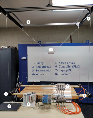
3.4. Real prototype

Finally, Figure 5 shows the prototype using a Beckhoff CX5130 industrial PC with distributed periphery connected by an EtherCAT Fieldbus to compact servo-drives terminals (EL7211) and four compact servo-motors with holding brakes (AM8112). The servo-drives were connected to the motors using OCT cables (One Cable Technology), which transmit both the electrical power to the motors and the position feedback signals from the encoders via the same cable. The default cycle times for the PLC and NC tasks were 10 ms and 2 ms respectively. The CDPR was programmed in Structured Text language according to IEC 61131–3 (IEC 2013). The following table shows the measurements used in the prototype.

Figure 5. Mechanical and electronics elements of the CDPR prototype.

4. Experimental evaluation and results

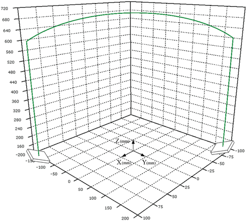
To execute tests on the proposed environment, an arbitrary Pick & Place trajectory, which is a very common operation with this type of robot, was performed. This trajectory was composed of a straight upward section, a curved section (arc of circumference), and a straight downward section (Figure 6). The trajectory was performed at two speeds of 100 and 500 mm/s with an acceleration of 3000 mm/s² and a jerk of 8000 mm/s³.

Figure 6. Three-dimensional pick & place trajectory for testing.

Three experiments were carried out. The first one focused on testing the computing time of three different methods for the direct kinematics calculation. The second one focused on the previously mentioned problem of reaction time between the setpoints generated in the PLC and the position feedback of the axes of the simulated model and the real prototype. Finally, in the last experiment, the trajectory performed by both systems was tracked and the errors regarding the original trajectory were analysed. The results and discussion of each experiment are shown below.

4.1. Real-time direct kinematics

This test evaluates the response of three direct kinematic calculation methods to determine the fastest one in feedbacking the current motor position. These three methods were: (1) the sphere intersection method explained in section 2.4 based on (Aflakian et al. 2018); (2) the Newton-Raphson numerical method applied to an industrial controller limiting it to three degrees of freedom (Silva, Garrido, and Riveiro 2022); (3) and a function block provided by the industrial controller manufacturer in a built-in library (Automation GmbH and KG 2023). The code implementing methods (1) and (2) for calculating the direct kinematics can be found in the open Github repository (Garrido Campos et al. 2024).

Table 2 shows the direct kinematic solution of an arbitrary point using these methods. The calculated position column shows all of them were able to calculate the robot current position with a variation of less than 10⁴ mm between them, showing their high accuracy response.

Table 2. Direct kinematic solution of an arbitrary point on the trajectory.

Method Pos	1- Spheres	2- Newton-Raphson	3- Built-in library
X	99.99992488	99.99994526	99.99993776
Y	−174.9999118	−174.999993	−175.0000312
Z	302.8803513	302.8803597	302.880296

Table 3 shows the computing time of the methods applied during the calculation of the previously exposed trajectory at the speed of 500 mm/s. To measure the computing time, the built-in ‘Profiler’ function block (Rupprecht, Vogel-Heuser, and Neumann 2023) was used to measure the CPU execution time at a given instant of the process. Therefore, calls were made to the ‘FB_Profiler’ immediately before and after the implemented direct kinematics resolution methods were executed.

Table 3. Comparison of computing time of direct kinematic methods to obtain a new solution.

N	Method	Average [us]	Minimum [us]	Maximum [us]	Number of program cycles to obtain a new solution
1	Spheres	17.52	17	19	1
2	Newton Raphson	32.31	17	41	1
3	Built-in library	18.28	17	20	4

From these results it can be seen that the geometric methods are especially faster in finding the direct kinematic solution, in contrast to the numerical method. Although the function in the built-in library (provided by the industrial controller manufacturer) is as fast as the method of the sphere intersection, it needs four program cycles to get a new solution. Therefore, the three-sphere intersection algorithm were the best option when implemented in the structural text programming language from the IEC 61131–3 standard.

As a discussion of the first test, the built-in library provides powerful tools to support the automation of spatial under-constrained CDPR of three and four cables, and therefore, extends the use of these robots in industry. Also, this library uses the same FB to calculate direct and inverse kinematics and their implementation follows the state machine defined by PLCopen for reusable Function Blocks, simplifying efforts to automate the robots. Nonetheless, having a state machine structure entails different intermediate states until a position calculation is done, making each position reading available only after a wait of a few cycles (in this case four cycles), as shown in Table 3. This drawback could be not enough for corrective actions in which knowing the position in a single PLC cycle is a critical factor. Finally, the Newton-Raphson numerical method is the worst performing one because it inherently involves iterations that entail more operations than the others.

4.2. Reaction time

In the second test, the axis positions of the simulated model (CoppeliaSim) and the industrial prototype (real motors) were compared with the commanded positions of the axes (industrial PLC controller). To perform this test, a movement was initiated in the industrial controller and the length value of each cable was monitored. The cable length values were stored at each cycle in an array for further processing. This was done against the simulated model and then against the real prototype. Therefore, the reaction time in the execution of the trajectories at two different speeds, 100 mm/s and 500 mm/s, can be observed. Figure 7 shows the trajectory execution for one of the cables at different speeds in both systems.

Figure 7. Reaction time difference between the position of the simulated and prototype axes with respect to the target position. a) simulated axis 1 and b) prototype axis 1 at slow speed. c) simulated axis 1 and d) prototype axis 1 at high speed.

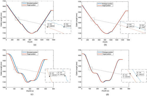
Figure 7a indicates that the simulated axes reproduce the target trajectory, and their motion also corresponds to that of the real axes of the prototype (Figure 7b), despite the relative delay between the systems. It has been observed that at 100 mm/s, the reaction time obtained for the axes of motion involved is 11 program cycles (that is, PLC task cycles) for the simulated case and two program cycles for the prototype motion case. Repeating the test at 500 mm/s (Figure 7c–d), the results show a difference in the reaction time of 18 program cycles for the simulated case and two program cycles for the prototype motion case. The raw data can be consulted in the supplementary information, as well as the graphs for the remaining axes.

In the case of the real prototype, the reaction time remains constant at two program cycles because the communication between the industrial controller and the servo-drives communicates via EtherCAT. This protocol is synchronous and deterministic, so it ensures that the new data will always be transmitted at the same time. In the case of the simulated model, however, it is necessary to consider that several agents are involved, in this case, a local network ADS communication from the PLC to the PC with the Python script, and internally, from the same PC to the simulator via WebSocket TCP. WebSocket TCP is not a synchronous and deterministic protocol, so it is not possible to ensure that the data obtained always takes the same time to be delivered. Analysing the change in the reaction time of the simulated model, this can be explained by the increase in speed, which involves four axes, making the dynamic simulator have to deal with a greater number of setpoints. These extra calculations make the system take longer to respond and thus affect its ability to start the movement in a fluid way.

4.3. Position error during a path motion

The third test evaluated the simulated model and industrial prototype end-effector position against the target position while executing the trajectory specified previously to compare the simulated model and prototype trajectory execution. To perform this test, the movement of the specified trajectory was started, the direct kinematics was performed by the sphere method in each program cycle, and the resulting data was stored in an array for further processing. Figure 8 shows the trajectory performed by the simulated model (simulator), real prototype and target setpoints for both speeds studied. The raw data can be consulted in the supplementary information.

Figure 8. Trajectories of the prototype, simulator, and target at two different speeds. Subfigures (a–c) show trajectories at 100 mm/s, and (d–f) at 500 mm/s, across X-Z, Y-Z, and X-Y planes, respectively.

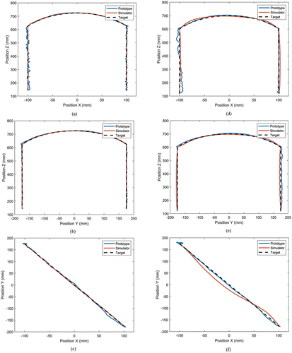
To analyse the error in the trajectory execution, the Euclidean distance between the corresponding points of the trajectory commanded and the one realized by the robot (simulated model and real prototype) was calculated. The trajectory was also segmented into three sections, straight upwards, displacement, and straight downwards to obtain the specific error in each phase of the movement, with straight and circular movements (circumferential arcs, in this case). Table 4 provides a detailed comparison between the errors of the simulated and actual prototype trajectories against the specified target trajectory, which travels in the three segments at speeds of 100 mm/s and 500 mm/s.

Table 4. Absolute error metrics during trajectory execution.

Phase/Segment	Parameters	Speed
		100 mm/s		500 mm/s
		Simulated	Prototype	Simulated	Prototype
Straight upwards	Average [mm]	0.712	2.364	5.148	6.447
	Standard deviation [mm]	0.403	1.253	3.161	3.815
	Max [mm]	3.085	6.485	14.080	13.225
	Min [mm]	0.028	0.004	0.004	0.008
Displacement	Average [mm]	1.521	2.996	8.087	8.517
	Standard deviation [mm]	0.923	1.692	4.898	2.787
	Max [mm]	7.392	6.865	18.596	14.579
	Min [mm]	0.000	0.152	0.002	3.940
Straight downwards	Average [mm]	0.730	1.312	4.788	4.865
	Standard deviation [mm]	0.468	0.593	3.336	2.708
	Max [mm]	2.862	3.800	13.181	8.219
	Min [mm]	0.000	0.156	0.000	0.385
Complete	Average [mm]	0.979	2.200	5.888	6.504
	Standard deviation [mm]	0.737	1.431	4.065	3.480
	Max [mm]	7.392	6.865	18.596	14.579
	Min [mm]	0.000	0.004	0.000	0.008

The experimental analysis shows that the prototype’s trajectory at 100 mm/s has consistently higher errors in all movement phases compared to the simulation, with the straight upwards phase particularly showing a prototype error more than three times the simulated error. The prototype’s trajectory also demonstrated more variability across all phases compared to the simulation, as shown by higher standard deviation values. Finally, Table 2 shows a similar pattern of standard deviation between the simulated and the prototype trajectory.

At a higher speed of 500 mm/s, the experimental data presents a narrower gap than the lower speed test for the average errors between the prototype and the simulated trajectories. The prototype’s average error slightly exceeds the simulation in all phases, but shows greater consistency, especially in the displacement segment, in which its standard deviation is lower than the simulated one. Also, unlike the situation at the lower speed, the average errors were much closer.

Analysing and discussing the data in Table 4, there is a consistency in the higher errors and variability in the prototype trajectory compared to the simulated trajectory in all sections and speeds. This could be due to several factors not modelled in the simulation, such as friction and other nonlinearities inherent to the real system. The straight downward phase shows the least discrepancy between the prototype and the simulation, suggesting that gravity helps to correct the trajectory, which can be observed in the closely aligned paths in Figure 8. This behaviour is the same regardless of the speeds tested. Although straight upwards and downwards are rectilinear motion, the first one started from the object at complete rest and had to go upwards (against gravity), which makes any misalignment in the prototype mechanics compromise the accuracy, for example between the winch and motor shaft. This is not noticeable in the simulated environment since a simplification of the cable pulling and pushing system with the two prismatic joints was used. Furthermore, the system is less accurate when performing straight arcs, as can be seen in Figure 8f. This is also influenced by the fact that it involves 3D motion, whereas ascending and descending segments start from more favourable initial conditions and only operate within a 2D plane.

In contrast with existing literature, a simulation and prototype of a 4-cable CDPR were conducted using SimulationX software (Jomartov et al. 2023), moving a punctual mass of 10 kg at 100 mm/s with hybrid stepper motors. For a circular trajectory in a 2D plane, approximate errors of 0.67 mm in X, 2.5 mm in Y, and 4.8 mm in Z between the simulated and executed were found. In the case of this research, the 4-cable CDPR with industrial servo-motors moved a rectangular mass of 0.602 kg at 100 mm/s for a 3D trajectory, obtaining maximum error values of 0.567 mm in X-Y when performing the circular arc movement, and 3.4 mm in Z when performing the ascent segment. The results obtained can be comparable to those reported by Jomartov et al. (2023), although performing a different trajectory.

Finally, the metric of ‘Mean Relative Position Error’ was calculated to assess the accuracy of both the simulated model and the prototype model in relation to the commanded model along the three-dimensional trajectory. In this way, an overall view of the system’s performance was obtained (Table 5). It is noteworthy that although the absolute errors increase with speed, the difference between the relative errors of the simulated and real prototype diminishes, decreasing from 0.27% to 0.15%.

Table 5. Mean relative position error during trajectory execution.

Velocity [mm/s]	Mean Relative Position Error [%]
	Simulated	Prototype	Error difference
100	0.19	0.46	0.27
500	1.27	1.42	0.15

Table 5 summarizes these results and shows that although the real prototype tended to have a higher relative error compared to the simulated model, the discrepancy between the two decreased as the speed increased. However, it is important to note that even the largest discrepancy in relative error at 100 mm/s is less than half a percentage point, indicating a satisfactory level of consistency between the simulated and real prototype robot.

These results together reinforce the usefulness of the simulator as a suitable tool for the design and initial validation of motion execution on CDPRs. Specifically, it is useful for performing pick & place tasks in an obstacle-free environment, where achieving the points of interest is more crucial than faithfully reproducing the trajectory. However, in comparison to other environments for the design, development, and control of CDPRs mentioned in section 1, the proposed environment allows to govern the simulation with the actual industrial controller that will be used in the final CDPR system.

5. Conclusions

The presence of Cable-Driven Parallel Robots in industrial applications is growing due to their inherent characteristics such as modularity, high payload-to-weight ratio, and the ability to operate in large workspaces. In this context, the development of a simulator designed to assist in both the early design stages and initial operational tests offers a clear advantage for the development of new CDPRs. This is because the simulator employs the same control and trajectory planning algorithms that would be used in the real robot, thereby enhancing the reliability of the process. Thus, this paper presents this integrated simulation and control environment as an additional tool to the existing ones for the CDPR design and development.

Experimental results revealed that the simulation accurately replicated the performance of the real prototype, both at 100 mm/s and 500 mm/s. Also, it should be highlighted that the system’s accuracy is notably higher at lower speeds against the target trajectory, suggesting that the implemented trajectory is especially efficient in these segments. Moreover, a maximum low deviation of 0.27% between the position of the simulated model and the real prototype was found under various speed scenarios, despite the difference in the reaction time between both systems. These deviations can be attributed to the inherent complexities of the dynamics in the real prototype that were not considered in the simulation. Additionally, different methods for calculating real-time direct kinematics for this type of robot with industrial controllers were implemented and compared. Although this is a well-known problem, the choice of one method over another is significant when it comes to executing trajectory-tracking control actions. In summary, the presented environment serves as a reliable tool for development and validation, closely replicating target movements. This utility enables a safer and less uncertain initial start-up for such fast-paced developments.

However, this study has certain limitations. Whilst using CoppeliaSim provides a realistic simulation, it cannot capture all the complexities of the real prototype. This includes factors such as mechanical wear, slippage of the cables with the pulleys, manufacturing inaccuracies in 3D-printed parts and their fit with motor shafts, which could account for some of the discrepancies observed in the results.

In future work, a more complex winding system will be incorporated to the simulation environment, as well as a more elaborated representation of the cables considering the catenary effect due to their mass, and the elasticity. To achieve this, the newly released CoppeliaSim-Mujoco feature for simulating non-rigid cables and soft bodies could be employed, although this would significantly increase the simulator’s development time. Additionally, the system’s performance will be explored using a CDPR model with more cables; increasing from four to eight cables to study their influence on precision and stability. The integration of obstacle-avoidance control strategies will also be tested in the environment, which is relevant for pick-and-place applications in complex industrial cases. Finally, the environment is being arranged to be used in the development and testing of a spatial CDPR robot for other non-industrial applications, such as marine cargo transfer between ships or gait rehabilitation, with an emphasis on controlling the interaction of the CDPR with objects and people.

Acknowledgments

The work of D. Silva-Muñiz has been supported by the 2023 predoctoral grant of the University of Vigo (00VI 131 H 6410211).

Supplementary material

Supplemental data for this article can be accessed online at https://doi.org/10.1080/0951192X.2024.2348499.

Disclosure statement

No potential conflict of interest was reported by the author(s).

References

- Aflakian, A., A. Safaryazdi, M. Tale Masouleh, and A. Kalhor. 2018. “Experimental Study on the Kinematic Control of a Cable Suspended Parallel Robot for Object Tracking Purpose.” Mechatronics 50 (April): 160–176. https://doi.org/10.1016/j.mechatronics.2018.02.005.
- Alias, C., I. Nikolaev, E. Garduno Correa Magallanes, and B. Noche. 2018. ‘An Overview of Warehousing Applications Based on Cable Robot Technology in Logistics’. In 2018 IEEE International Conference on Service Operations and Logistics, and Informatics (SOLI), 232–239. Singapore: IEEE. https://doi.org/10.1109/SOLI.2018.8476760.
- Automation GmbH, B., and C. KG. 2023. ‘Fb_kincalctrafo’. Manual. Tf511x | TwinCAT 3 Kinematic Transformation. Accessed September 12. https://infosys.beckhoff.com/english.php?content=./content/1033/tf5110-tf5113_tc3_kinematic_transformation/1955795083.html&id=.
- Chawla, I., P. M. Pathak, L. Notash, A. K. Samantaray, Q. Li, and U. K. Sharma. 2023. “Inverse and Forward Kineto-Static Solution of a Large-Scale Cable-Driven Parallel Robot Using Neural Networks.” Mechanism and Machine Theory 179 (January): 105107. https://doi.org/10.1016/j.mechmachtheory.2022.105107.
- Collins, J., S. Chand, A. Vanderkop, and D. Howard. 2021. “A Review of Physics Simulators for Robotic Applications.” IEEE Access 9:51416–51431. https://doi.org/10.1109/ACCESS.2021.3068769.
- Garrido Campos, J., D. Silva-Muñiz, J. Rivera-Andrade, and E. Riveiro. 2024. Cdpr_4cables_kinematics_library. Github. https://github.com/laboratoriorma3/CDPR_4cables_kinematics_library.
- González-Rodríguez, A., A. Martín-Parra, S. Juárez-Pérez, D. Rodríguez-Rosa, F. Moya-Fernández, F. J. Castillo-García, and J. Rosado-Linares. 2023. “Dynamic Model of a Novel Planar Cable Driven Parallel Robot with a Single Cable Loop.” Actuators 12 (5): 200. https://doi.org/10.3390/act12050200.
- Hussein, H., J. Cavalcanti Santos, J.-B. Izard, and M. Gouttefarde. 2021. “Smallest Maximum Cable Tension Determination for Cable-Driven Parallel Robots.” IEEE Transactions on Robotics 37 (4): 1186–1205. https://doi.org/10.1109/TRO.2020.3043684.
- IEC. 2013. “Programmable Controllers-Part 3: Programming Languages.” In Standard IEC 61131-3:2013, Geneva, Switzerland: ISO. https://webstore.iec.ch/publication/4552.
- Izard, J.-B., D. Alexandre, H. Pierre-Elie, E. Cabay, C. David, R. Mariola, and B. Mikel. 2018. “On the Improvements of a Cable-Driven Parallel Robot for Achieving Additive Manufacturing for Construction.” In Cable-Driven Parallel Robots, edited by C. Gosselin, P. Cardou, T. Bruckmann, and A. Pott, 353–363. Vol. 53 Mechanisms and Machine Science. Cham: Springer International Publishing. https://doi.org/10.1007/978-3-319-61431-1_30.
- Jomartov, A., A. Tuleshov, A. Kamal, and A. Abduraimov. 2023. “Simulation of Suspended Cable-Driven Parallel Robot on SimulationX.” International Journal of Advanced Robotic Systems 20 (2): 172988062311614. https://doi.org/10.1177/17298806231161463.
- Kalajahi, E. G., M. Mahboubkhah, and A. Barari. 2021. “Numerical versus Analytical Direct Kinematics in a Novel 4-DOF Parallel Robot Designed for Digital Metrology.” IFAC-Papersonline 54 (1): 181–186. https://doi.org/10.1016/j.ifacol.2021.08.021.
- Lau, D., J. Eden, Y. Tan, and D. Oetomo. 2016. ‘CASPR: A Comprehensive Cable-Robot Analysis and Simulation Platform for the Research of Cable-Driven Parallel Robots’. In 2016 IEEE/RSJ International Conference on Intelligent Robots and Systems (IROS), 3004–3011. Daejeon, South Korea: IEEE. https://doi.org/10.1109/IROS.2016.7759465.
- Lehmann, S. 2023. ‘Https://Pypi.Org/Project/Pyads/’ Accessed September 12. https://pyads.readthedocs.io/en/latest/index.html#.
- McDonald, E., B. Steven, and A. Marc. 2022. “CDPR Studio: A Parametric Design Tool for Simulating Cable-Suspended Parallel Robots.” In Computer-Aided Architectural Design. Design Imperatives: The Future is Now, edited by D. Gerber, E. Pantazis, B. Bogosian, A. Nahmad, and C. Miltiadis, 344–359. Vol. 1465 Communications in Computer and Information Science. Singapore: Springer Singapore. https://doi.org/10.1007/978-981-19-1280-1_22.
- Mersi, R., S. Vali, M. Shahamiri Haghighi, G. Abbasnejad, and M. Tale Masouleh. 2018. ‘Design and Control of a Suspended Cable-Driven Parallel Robot with Four Cables’. In 2018 6th RSI International Conference on Robotics and Mechatronics (IcRoM), 470–475. Tehran, Iran: IEEE. https://doi.org/10.1109/ICRoM.2018.8657534.
- Pan, W., K. Iturralde Lerchundi, R. Hu, T. Linner, and T. Bock. 2020. “Adopting Off-Site Manufacturing, and Automation and Robotics Technologies in Energy-Efficient Building.” Kitakyushu, Japan: https://doi.org/10.22260/ISARC2020/0215
- Pessoa De Melo, S., J. G. D. S. N. Mirella, P. Jorge Lima Da Silva, J. Marcelo Xavier Natario Teixeira, and V. Teichrieb. 2019. ‘Analysis and Comparison of Robotics 3D Simulators’. In 2019 21st Symposium on Virtual and Augmented Reality (SVR), 242–251. Rio de Janeiro, Brazil: IEEE. https://doi.org/10.1109/SVR.2019.00049.
- Phanden, R. K., P. Sharma, and A. Dubey. 2021. ‘A Review on Simulation in Digital Twin for Aerospace, Manufacturing and Robotics’. Materials Today: Proceedings 38: 174–178. https://doi.org/10.1016/j.matpr.2020.06.446.
- Pott, A. 2019. “WireX – An Open Source Initiative Scientific Software for Analysis and Design of Cable-Driven Parallel Robots.” Unpublished. https://doi.org/10.13140/RG.2.2.25754.70088.
- Qian, S., B. Zi, W.-W. Shang, and Q.-S. Xu. 2018. “A Review on Cable-Driven Parallel Robots.” Chinese Journal of Mechanical Engineering 31 (1): 66. https://doi.org/10.1186/s10033-018-0267-9.
- Robotics, C., Ltd. 2023a. ‘Dynamics’. Accessed September 11. https://www.coppeliarobotics.com/helpFiles/en/dynamicsModule.htm.
- Robotics, C., Ltd. 2023b. ‘Remote API Modus Operandi’. Accessed September 12. https://www.coppeliarobotics.com/helpFiles/en/remoteApiModusOperandi.htm.
- Robotics, C., Ltd. 2023c. ‘Robot Simulator CoppeliaSim: Create, Compose, Simulate, Any Robot - Coppelia Robotics’. Accessed September 11. https://www.coppeliarobotics.com/.
- Rodriguez-Barroso, A., M. Khan, V. Santamaria, E. Sammarchi, R. Saltaren, and S. Agrawal. 2023. “Simulating Underwater Human Motions on the Ground with a Cable-Driven Robotic Platform.” IEEE Transactions on Robotics 39 (1): 783–790. https://doi.org/10.1109/TRO.2022.3197338.
- Rupprecht, B., B. Vogel-Heuser, and E.-M. Neumann. 2023. ‘Measurement Methods for Software Execution Time on Heterogeneous Edge Devices’. In 2023 IEEE 21st International Conference on Industrial Informatics (INDIN), 1–6. Lemgo, Germany: IEEE. https://doi.org/10.1109/INDIN51400.2023.10218136.
- Silva, D., J. Garrido, and E. Riveiro. 2022. “Stewart Platform Motion Control Automation with Industrial Resources to Perform Cycloidal and Oceanic Wave Trajectories.” Machines 10 (8): 711. https://doi.org/10.3390/machines10080711.
- Song, D., X. Xiao, G. Li, L. Zhang, F. Xue, and L. Li. 2023. “Modeling and Control Strategy of a Haptic Interactive Robot Based on a Cable-Driven Parallel Mechanism.” Mechanical Sciences 14 (1): 19–32. https://doi.org/10.5194/ms-14-19-2023.
- South African Instrumentation and Control. 2008. ‘Spectacular Television Images: Beckhoff Embedded PCs Control SpiderCam Camera Robot - August 2008 - Beckhoff Automation - SA Instrumentation & Control’. PLCs, DCSs & Controllers. Spectacular Television Images: Beckhoff Embedded PCs Control SpiderCam Camera Robot. https://www.instrumentation.co.za/news.aspx?pklnewsid=29682.
- Tič, V., and D. Lovrec. 2022. “Development and Implementation of Closed Loop Position Control Concepts on Electromechanical Linear System Using Beckhoff Controller.” Machines Technologies Materials 16 (4): 116–119. ( Scientific Technical Union of Mechanical Engineering” Industry 4.0).
- Weber, A., E. Holger, S. Per, and W. Svenja. 2023. “Performance Comparison of TwinCat ADS for Python and Java.” In Softwaretechnik-Trends Band 43, Heft 4, edited by A. Herrmann. Gesellschaft für Informatik e.V. https://dl.gi.de/handle/20.500.12116/43230.
- Zake, Z., C. Stéphane, S. R. Adolfo, C. François, and P. Nicolò. 2019. “Stability Analysis of Pose-Based Visual Servoing Control of Cable-Driven Parallel Robots.” In Cable-Driven Parallel Robots, edited by A. Pott and T. Bruckmann, 73–84. Vol. 74 Mechanisms and Machine Science. Cham: Springer International Publishing. https://doi.org/10.1007/978-3-030-20751-9_7.
- Zarebidoki, M., J. Singh Dhupia, and W. Xu. 2022. “A Review of Cable-Driven Parallel Robots: Typical Configurations, Analysis Techniques, and Control Methods.” IEEE Robotics & Automation Magazine 29 (3): 89–106. https://doi.org/10.1109/MRA.2021.3138387.
- Zhang, Z., Z. Shao, Z. You, X. Tang, B. Zi, G. Yang, C. Gosselin, and S. Caro. 2022. “State-Of-The-Art on Theories and Applications of Cable-Driven Parallel Robots.” Frontiers of Mechanical Engineering 17 (3): 37. https://doi.org/10.1007/s11465-022-0693-3.
- Zhang, T., Y. Shi, Y. Cheng, Y. Zeng, X. Zhang, and S. Liang. 2023. “The Design and Implementation of Distributed Architecture in the CMOR Motion Control System.” Fusion Engineering and Design 186 (January): 113357. https://doi.org/10.1016/j.fusengdes.2022.113357.