Can system reliability be predicted from average component reliabilities?

Abstract

The paper reveals that a prediction of system reliability on demand based on average reliabilities on demand of components is a fundamentally flawed approach. A physical interpretation of algebraic inequalities demonstrated that assuming average component reliabilities on demand entails an overestimation of the system reliability on demand for systems with components logically arranged in series and series-parallel and underestimation of the reliability on demand for systems with components logically arranged in parallel. The key reason for these discrepancies is the variability of components from the same type. Techniques for countering variability by promoting asymmetric response through inversion have also been introduced. The paper demonstrates that variability during assembly operations can affect negatively the reliability of mechanical systems. Accordingly, techniques for reducing the variability of stresses during assembly operations have been discussed. Finally, the paper provides a discussion related to the reasons for the relatively slow adoption of domain-independent methods for improving reliability despite their numerous advantages.

Keywords:

• Variability
• system reliability
• increasing the level of balancing
• domain-independent methods

1. Introduction

Although reliability and risk assessment have been recognised as domain-independent areas (Aven, 2016; Henley & Kumamoto, 1981; Kaplan & Garrick, 1981; Vose, 2000), the same cannot be said for the equally important areas of reliability improvement and risk reduction. For many years, the reliability and risk literature (Dhillon, 2017; Ebeling, 1997; Gullo & Dixon, 2018; Henley & Kumamoto, 1981; Hoyland & Rausand, 1994; Lewis, 1966; Modarres et al., 2016; O’Connor, 2002; Ramakumar, 1993; Vose, 2000) failed to acknowledge and highlight the fact that reliability improvement and risk reduction are underpinned by general principles that work across diverse domains.

Standard textbooks on mechanical engineering and design of machine components (such as Hearn, 1985; Matthews, 1998; Samuel & Weir, 1999; French, 1999; Thompson, 1999; Gere & Timoshenko, 1999; Collins, 2003; Norton, 2006; Pahl et al., 2007; Childs, 2014; Budynas, 1999; Budynas & Nisbett, 2015; Mott et al., 2018; Gullo & Dixon, 2018) also provide very little discussion on generic (domain-independent) methods for reliability improvement and risk and uncertainty reduction.

An important contributing factor for the apparent insufficient attention to domain-independent approaches for enhancing reliability was the excessive emphasis on reliability prediction methodologies, specifically those associated with estimating system reliability using average component reliabilities. To achieve this, average failure rates of components were sourced from various reliability databases (e.g. MIL-STD-1629A, 1977). System reliability for very complex systems was calculated on the basis of the average failure (hazard) rates of the components building the systems. The shortcomings of this approach in generating accurate system reliability predictions led to growing disillusionment among researchers and practitioners. As a result, some authors (Knowles, 1993) questioned the validity of failure rate-based reliability predictions. Furthermore, the reliability on demand of a vast range of systems was based on the average reliability on demand of the components building the systems. Consequently, Section 2 of this article explores some of the reasons behind the failure of methods reliant on average component reliabilities on demand to accurately predict system reliability on demand.

A compilation and analysis of common mistakes in design that led to catastrophic failures has been presented in Petroski (1994). Domain-independent methods for improving reliability in design have been presented in Todinov (2019). Despite the clear advantages provided by the domain-independent methods for improving reliability, these methods have not been widely used to inform the design process.

French (1999), for example, formulated several general principles for conceptual design. However, these principles did not focus on enhancing reliability or reducing technical risk. Pahl et al. (2007) also discussed general principles for engineering design. Yet, many of these principles either do not emphasise improving reliability and minimising risk or are overly specific (e.g. the principle of thermal design) and lack broad applicability. Collins (2003) explored engineering design from a failure prevention perspective, but no risk-reducing methods or principles with universal applicability were formulated.

Thompson (1999) highlighted the necessity of effectively integrating maintainability and reliability considerations into the design process and emphasised the significance of failure mode and effects analysis (FMEA) in design. While the FMEA, which is widely used in the industry, is valuable for understanding how a component’s malfunction can lead to system failure, it does not provide much guidance on domain-independent principles for designing for reliability.

Another problem is that the current approach to reliability improvement and risk reduction is almost entirely reliant on domain-specific knowledge and is conducted solely by experts in those domains.

The TRIZ problem-solving framework (Altshuller, 1984, 1999), widely adopted by companies and researchers around the world (Orloff, 2006; Rantanen & Domb, 2008; Terninko et al., 1998), clearly demonstrated the advantages of using generic principles in resolving technical contradictions and driving innovation.

By using domain-independent methods, rapid mental mapping can be achieved for challenging problems, thereby bolstering intuition. This often leads to surprising breakthroughs and swift outcomes. Take, for instance, the domain-independent principle of inversion (Todinov, 2019). Understanding this principle often leads to innovative approaches in improving reliability involving reversing position, motion direction, properties, features, states, or thought processes. A failure mode that appears in a specific position, orientation, motion, state, or property often vanishes when the position, orientation, motion or state is shifted to the opposite one while maintaining the system’s essential functions.

The domain-independent method of algebraic inequalities (Todinov, 2023), for example, can be used for improving the reliability of any series-parallel system by asymmetric permutation of interchangeable redundancies even when the reliabilities of individual components are unknown.

The effectiveness of the domain-independent principles in improving reliability lies in the fact that solutions to reliability issues in one domain can be applied to other domains by using the same principle. For example, the problem of premature failure of one of several power transistors working in parallel can often be solved by the domain-independent principle "increasing the level of balancing", through more uniform distribution of the electrical load across the transistors. The same principle can be used to achieve a uniform load distribution along the thread of bolted joints (Coria et al., 2020) and to eliminate premature failure of a shaft-hub connection based on a single key. The last issue can be addressed by replacing the key with splines, which also increases the level of balancing and distributes the load more uniformly. The same principle can also be used to eliminate damaging the top of a pile driven into the ground by introducing an intermediate component that distributes the load more evenly (Orloff, 2006).

Despite the clear advantages of the domain-independent principles for improving reliability, their adoption has been relatively slow. This can be attributed to a number of factors.

The first contributing factor is the lack of awareness and education regarding these principles. Reliability engineers, as well as other professionals involved in reliability improvement, are still unaware of the potential benefits from using the domain-independent methods. There is a lack of educational resources and training programs available to help individuals and organisations learn about these methods and develop the necessary skills to implement them.

The traditional reliability engineering education programs have not yet incorporated these methods into their curriculum, leading to a gap in knowledge and skills among practicing engineers.

Another contributing factor is that reliability improvement has traditionally relied upon methods such as active, standby, and k-out-of-n redundancy, physics-of-failure approach, as well as strengthening the design by incorporating various types of reinforcement, selecting stronger or corrosion-resistant alloys and condition monitoring. These techniques have been established and refined over many years and are familiar to reliability engineers and other professionals in the field. However, while useful in a number of cases, these techniques are associated with high implementation costs. These well-known methods created resistance to change, particularly for those who have become accustomed to relying on a small set of well-known, albeit costly techniques. In contrast, many domain-independent methods, such as the method of inversion for example, are not normally associated with significant implementation costs.

A strong reason for the slow adoption of domain-independent methods for reliability improvement is the belief held by many engineers that their specialised knowledge and expertise in their field is sufficient to solve all reliability issues associated with their designs. These engineers often view domain-independent methods as less tailored in addressing the specific reliability issues within their narrow domain and for that reason they view these methods as less effective. As a result, they remain attached to their established methods, despite the potential benefits that domain-independent methods offer. This leads to mental inertia caused by conventional wisdom, tradition and entrenched beliefs. Comprehensive knowledge of a specific domain often hinders innovation. It makes domain experts resist novel ideas in their domains and limits the possibility to take advantage of novel approaches to reliability improvement, which could positively impact the reliability and safety of their designs.

Another reason for the slow adoption of domain-independent techniques is the prominence of the physics-of-failure approach (Pecht et al., 1990). This approach, which emphasises the development of models based on underlying failure mechanisms, has been embraced by many reliability practitioners as the only reliable way to achieve improved reliability. However, while this approach has undoubtedly led to improvements in reliability on numerous occasions, it is not always practical or feasible to rely exclusively on physics-of-failure models.

The physical mechanisms underlying failure modes can be extremely complex and difficult to understand, leading to a great deal of uncertainty. Additionally, in some cases, failures are the result of multiple contributing factors, making it difficult to identify the root causes. For instance, corrosion fatigue involves two complex interdependent and synergistic failure mechanisms, making it particularly challenging to understand.

Next, revealing the root causes of failure usually requires extensive research which is costly and time consuming. Thus, continuing the previous example, the complex mechanism of corrosion fatigue (Pao, 1996) cannot be captured and modelled effectively if limited research is done on corrosion, fatigue and their interaction.

Root cause analysis is usually based on collecting data and data collection is always associated with cost limitations. Acquiring the necessary reliable data capturing and quantifying different types of uncertainty is a difficult task which requires significant investment. Most importantly, physics-of-failure models, even when highly successful, cannot transcend the narrow domain they serve and cannot normally be used to improve reliability in another, unrelated domain.

In contrast, domain-independent principles, such as the principle of reducing the variability of reliability-critical parameters, take a more comprehensive and holistic approach to reliability improvement, considering common factors that impact performance.

In this regard, this paper explores in detail the impact of variability of reliability-critical parameters on predictions related to system reliability on demand. This is done through the domain-independent method of algebraic inequalities - through physical interpretation of the classical arithmetic mean – geometric mean (AM-GM) algebraic inequality (Steele, 2004) and a new algebraic inequality based on concave functions.

This paper also explores some domain-independent techniques for counteracting the variability of reliability-critical parameters.

2. The influence of variability in identical-type products on system reliability

2.1. Impact of variability on the product of quantities from the same type

The negative impact of variability on the product of quantities of the same type X, can be demonstrated by a physical interpretation of the arithmetic mean-geometric mean algebraic inequality.

Consider the well-known arithmetic mean-geometric mean (AM-GM) inequality (Steele, 2004): (1) $$\frac{x_1+x_2+\dots +x_n}{n}\ge \sqrt[n]{x_1{x}_2\dots x_n}$$(1) where $x_1,\dots ,x_n$ are n positive real values representing various measurements of a quantity of the same type X.

Inequality (1) has a useful physical interpretation if presented in the equivalent form (2). (2) $${\left(\frac{x_1+x_2+\dots +x_n}{n}\right)}^n\ge x_1{x}_2\dots x_n$$(2)

The right-hand side of inequality (2) then can be physically interpreted as the value of the product of n quantities of the same type X.

The expression $\overline{x}=\frac{x_1+x_2+\dots +x_n}{n}$ in the left-hand side of inequality (2) can be interpreted as the average quantity $\overline{x}$ of type X. It is simply obtained by taking the average of the measurements characterising the quantity X. Inequality (2) can also be rewritten as (3) $${\overline{x}}^n\ge x_1{x}_2\dots x_n$$(3)

The left-hand side of inequality (3) can be physically interpreted as a value of the product where each measurement has the same, average value $\overline{x}.$ Inequality (3) effectively states that the predicted magnitude of the product ${\overline{x}}^n$ based on an average estimate of the quantity of type X is higher than the actual value of the product from n separate measurements.

The larger the deviations of the quantity X from the average value $\overline{x}=\frac{x_1+x_2+\dots +x_n}{n},$ the stronger the inequality (3). Inequality (3) transforms into equality in case of no variation of the quantity X. In other words, for the perfectly balanced case, $x_1=x_2=\dots =x_n,$ the equality ${\overline{x}}^n=x_1{x}_2\dots x_n$ holds.

Here is an example. It is a well-established property that the overall gain (amplification factor) of multiple voltage amplifiers of the same type connected in series, with gains $x_1,x_2,\dots ,x_n$, is given by the product $x_1{x}_2\dots x_n$ of the gains of the individual multipliers. Thus, the gain of a cascade of n voltage amplifiers of the same type can be calculated by using the right-hand side of inequality (3) where $x_i$ is the measured gain of the ith amplifier or by averaging the gains of all amplifiers and using the average gain $\overline{x}.$ The gain of a cascade of n voltage amplifiers of the same type can also be estimated from the left-hand side of inequality (3) based on the average gain of the amplifiers. This estimate however, deviates significantly from the real value given by the right-hand side of inequality (3). Due to inherent variability, the measured gain for amplifiers of the same type will exhibit differences and using the average gain in calculations will result in a considerable deviation of the estimated amplification factor from the true amplification factor.

2.2. Reliability on demand predictions for systems whose components are logically arranged in series

To simplify the analysis in assessing the impact of component variability on predicting the system reliability on demand, only systems with components working independently from one another will be considered. The impact of assuming average reliability on demand on predicting the system reliability on demand will be investigated through a system with components which are: (i) logically arranged in series (Figure 1a), (ii) logically arranged in parallel (Figure 1b) and (iii) logically arranged in series-parallel (Figure 2a).

Figure 1. Reliability network of a system with components from n varieties, (a) logically arranged in series; (b) logically arranged in parallel.

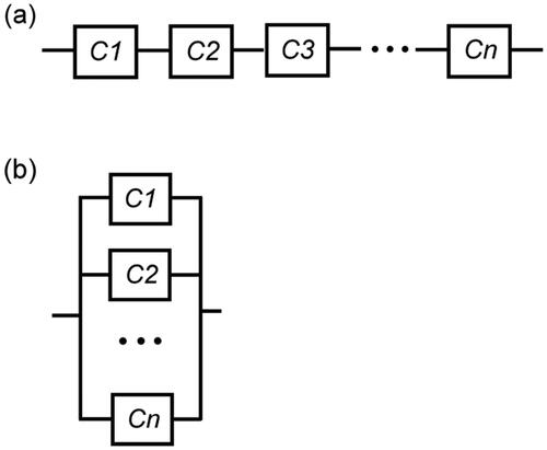
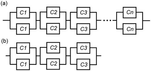
Figure 2. (a) Reliability network of a series-parallel system with components from n varieties; (b) reliability network of a series-parallel system involving components of 3 varieties.

Consider the section in Figure 1a including a number of components from the same type but of different variety, logically arranged in series and working independently of one another. Let $x_i$ ($0<x_i<1$) be the reliability on demand of a component $C_i$ of variety i, where $i=1,2,\dots ,n.$ The different component varieties $C_i$ can, for example, be associated with different suppliers, different working conditions, or different age.

The negative impact of variability on the predicted system reliability for the system in series, in Figure 1a can be demonstrated by a physical interpretation of the arithmetic mean-geometric mean algebraic inequality (2).

The right-hand side of inequality (2) can be physically interpreted as the reliability on demand of a section composed of n components of different variety, logically arranged in series (all components are of the same type).

The variables $x_i$ in inequality (2) represent the reliabilities on demand for components of different varieties, but all of the same type. Obtaining individual component reliabilities on demand for these different varieties is impractical. To do so would necessitate knowledge of the reliability on demand for every single component manufactured, for any age, working environment, duty cycle, number and type of material flaws, etc. This is why it is inevitable to use average values for predicting the reliability on demand of sections that contain components of the same type but of different varieties.

Due to differences in age, the presence of varying numbers of material and manufacturing flaws, inconsistencies in the manufacturing process, and variability in maintenance and working conditions, no two components of the same type have identical reliability. For example, the presence of material flaws significantly influences the reliability variation of components (Todinov, 2002, 2006). Thus, components of the same type and material, sourced from different suppliers, may exhibit considerable differences in their reliabilities. Such differences can be attributed to variations in the number, size, and location of inclusions and other imperfections within the high-stress zones of the components.

When dealing with n components of a particular type X, we are essentially dealing with a set of inhomogeneous components from n distinct varieties. Due to the impossibility of determining the reliability on demand that characterises these different varieties, this inherent inhomogeneity necessitates the use of the average component reliability on demand. For instance, if 639 out of 900 valves of type X respond to a command to close/open, the reliability on demand for valves of type X would be assessed by using the average value $639/900=0.71.$

The expression $\overline{x}=\frac{x_1+x_2+\dots +x_n}{n}$ in the left-hand side of inequality (2) can be interpreted as the average reliability on demand $\overline{x}$ of the components from the selected type, regardless of their variety. It is simply obtained by taking the average of the reliabilities on demand characterising the separate varieties. The left-hand side of inequality (2) can be physically interpreted as a reliability on demand of a section constructed with n components logically arranged in series where each component has the same, average reliability $\overline{x}.$ The right-hand part of inequality (2) is the actual reliability of the system in Figure 1a.

Inequality (2) effectively states that the predicted system reliability on demand based on an average component reliability on demand $\overline{x}$ is higher than the actual reliability on demand of the system.

The expression $\overline{x}=\frac{x_1+x_2+\dots +x_n}{n}$ in the left-hand part of (2) is the average reliability $\overline{x}$ on demand for the components from the selected type X (e.g. valve, sensor, seal, etc.), assessed as an average related to n varieties. Note that the reliabilities on demand $x_i$ characterising the n varieties are not known and this is why the system reliability on demand cannot be estimated by using these probabilities. Because the expression for $\overline{x}$ cannot be evaluated using $x_i,$ the ratio $p_r/p$ is used instead where $p_r$ is the number of successfully operating (reliable) components from type X, from past observations (statistics) and p is the total number of observed components.

Let us assume for simplicity, that the number of component varieties is equal to the number n of components. Thus, for the average reliability on demand $\overline{x}$ of components from type X, the following equation holds: (4) $$\overline{x}=\frac{x_1+x_2+\dots +x_n}{n}\approx \frac{p_r}{p}$$(4)

Equation (4)(4) $$\overline{x}=\frac{x_1+x_2+\dots +x_n}{n}\approx \frac{p_r}{p}$$(4) can be verified immediately considering that the left-hand side of (4) can be presented as (5) $$\frac{x_1+x_2+\dots +x_n}{n}=(1/n)\times x_1+(1/n)\times x_2+\dots +(1/n)x_n$$(5) which essentially represents the total probability associated with the successful operation of a component from type X. Indeed, a component from type X can operate successfully in n mutually exclusive ways. This includes the scenario where the component belongs to variety 1 and operates successfully (a compound event with probability $(1/n)x_1$), the scenario where the component belongs to variety 2 and operates successfully (a compound event with probability $(1/n)x_2$), and so on.

The probability of successful operation of the component must approach $p_r/p$ because this ratio is the empirical reliability on demand for the component.

Very similar reasoning also applies to the case where the number n of varieties is smaller than the number $n_c$ of components in the system ($n<n_c$). Indeed, let $n_1,n_2,\dots ,n_n$ (${\sum }_{i=1}^n{n}_i=n_c$) be the number of components in the system from each variety (these numbers are also unknown). The total probability of successful operation of a component in the system is then given by the left-hand side of (6): (6) $$\frac{n_1{x}_1+n_2{x}_2+\dots +n_n{x}_n}{n_c}=\frac{p_r}{p}$$(6) which must be equal to $p_r/p$ - the empirical probability of successful operation, where $p_r$ is the observed in the past total number of reliable components (from statistics) and p is the total number of observed components. The left-hand side of (6) is the weighted average of the probabilities of failure characterising the n varieties.

Indeed, a component in the system can operate successfully in n mutually exclusive ways. This includes the scenario where the component belongs to variety 1 and operates successfully (a compound event with probability $(n_1/n_c)x_1,$ the scenario where the component belongs to variety 2 and operates successfully (a compound event with probability $(n_2/n_c)x_2,$ and so on).

The total probability of a component operating successfully is then given by Equation (6)(6) $$\frac{n_1{x}_1+n_2{x}_2+\dots +n_n{x}_n}{n_c}=\frac{p_r}{p}$$(6) .

To test Equations (4)(4) $$\overline{x}=\frac{x_1+x_2+\dots +x_n}{n}\approx \frac{p_r}{p}$$(4) and (6)(6) $$\frac{n_1{x}_1+n_2{x}_2+\dots +n_n{x}_n}{n_c}=\frac{p_r}{p}$$(6) , Monte Carlo simulations were also performed, based on p = 100,000 observed components and n = 1,2,…,10, component varieties. In an array, random values between 0 and 1 are initially assigned for the probabilities of failure characterising the n varieties. Next, p = 100,000 components were selected by choosing randomly their variety. Each randomly selected component was also virtually tested for reliable operation on demand by using the reliability on demand characterising its variety. At the end of the simulation, the ratio of the total number of reliable components $p_r$ and the total number p = 100,000 observed components was formed. The validity of Equations (4)(4) $$\overline{x}=\frac{x_1+x_2+\dots +x_n}{n}\approx \frac{p_r}{p}$$(4) and (6)(6) $$\frac{n_1{x}_1+n_2{x}_2+\dots +n_n{x}_n}{n_c}=\frac{p_r}{p}$$(6) has been confirmed with each Monte Carlo simulation.

The discrepancy between the predicted and the actual system reliability on demand can be significant as the next numerical example demonstrates.

Let’s consider 900 valves of the same type X but of three different varieties (e.g., valves from machine centres 1, 2 and 3). From past statistics, 639 of the monitored 900 valves are reliable on demand. Because only the total number of valves 900 and the total number of reliable valves are known, the reliability on demand for the valves of type X will be estimated from: $$\overline{x}=639/900=0.71$$

Assume that a set of three valves on a pipeline are initially closed and must all open on command to allow fluid through the pipeline. This means that the set of valves are logically arranged in series (each valve must be operational for the system to be operational). Commonly, the reliability of the section consisting of these three valves is estimated on the basis of the average reliability on demand $\overline{x}$ characterising the valves. The reliability of the section is estimated from: $$R_{\mathit{\text{est}}}=0.71\times 0.71\times 0.71=0.36$$

Because of variability in component reliabilities on demand, the actual reliability on demand of the valve arrangement will be different from the estimated reliability on demand.

Considering the results (4) and (6), according to which (7) $$\overline{x}=\frac{p_r}{p}=\frac{x_1+x_2+\dots +x_n}{n}$$(7) inequality (3) can be rewritten as (8) $${(p_r/p)}^n\ge x_1\times x_2\times \cdots \times x_n$$(8)

Assume for the sake of simplicity, that 300 valves of type X have been manufactured from each of the 3 manufacturing centres (valves of three distinct varieties). Let the number of reliable valves from the different varieties be 288, 258 and 93, correspondingly.

Consequently, the reliability on demand for each variety is as follows: $x_1=288/300=0.96,$ $x_2=258/300=0.86$ and $x_3=93/300=0.31,$ correspondingly.

As can be verified, the following expression holds true for the average reliability on demand $\overline{x}:$ $$\overline{x}=(x_1+x_2+x_3)/3=(0.96+0.86+0.31)/3=0.71=p_r/p=639/900$$

Suppose that a valve from each variety has been used to construct the section of three valves, logically arranged in series.

The actual reliability on demand of the section with three valves is $$R_{\mathit{\text{real}}}=x_1\times x_2\times x_3=0.96\times 0.86\times 0.31=0.26$$

As can be verified, the following relationships hold for the reliability on demand for the valves of type X: $$\overline{x}=\frac{p_r}{p}=\frac{288+258+93}{900}=\frac{x_1+x_2+x_3}{3}=\frac{0.96+0.86+0.31}{3}=0.71$$

The estimated system reliability on demand ($R_{\mathit{\text{est}}}=0.36$), derived from the average component reliability on demand, is 1.38 times higher than the actual reliability on demand ($R_{\mathit{\text{real}}}=0.26$) of the section. The reason for this discrepancy is inequality (8).

Indeed, according to expression (6), the average reliability on demand is given by: $$\overline{x}=\frac{300\times x_1+300\times x_2+300\times x_3}{900}=\frac{x_1+x_2+x_3}{3}$$

According to inequality (8): $${(p_r/p)}^3\ge x_1{x}_2{x}_3$$

The larger the deviations of the reliabilities on demand characterising the different varieties from the average value $\overline{x}=\frac{p_r}{p}=\frac{x_1\hspace{0.17em}+\hspace{0.17em}{x}_2\hspace{0.17em}+\hspace{0.17em}\dots \hspace{0.17em}+\hspace{0.17em}{x}_n}{n},$ the stronger the inequality (8) will be. Inequality (8) transforms into equality in case of no variation of the reliabilities on demand characterising the separate varieties. In this case, $x_1=x_2=\dots =x_n$ and $${\left(\frac{x_1+x_2+\dots +x_n}{n}\right)}^n=x_1{x}_2\dots x_n$$

Indeed, assume again that the total number of monitored valves from type X is 900 and the statistics indicated that the number of reliable valves is 639.

Because only the total number of observed valves 900 and the total number of observed reliable valves are known, the reliability on demand of the valve from type X will be estimated from: $$\overline{x}=639/900=0.71$$

Assuming that the valves in the section are logically arranged in series, the reliability of the section is estimated from $$R_{\mathit{\text{est}}}=0.71\times 0.71\times 0.71=0.36$$

Let the number of reliable valves characterising the different varieties be close values, with small variation: 230, 210 and 199, correspondingly. In this case, the reliabilities on demand characterising the different varieties are: $x_1=230/300=0.77,$ $x_2=210/300=0.70$ and $x_2=199/300=0.66,$ correspondingly. Suppose again, that a valve from each variety has been used to construct the section of three valves where the valves are logically arranged in series.

The real reliability of the section is then $$R_{\mathit{\text{real}}}=x_1\times x_2\times x_3=0.77\times 0.7\times 0.66=0.35$$ which is now very close to the estimated value $R_{\mathit{\text{est}}}=0.36$ of the reliability on demand for the section.

If there were no variability in the reliabilities of components of the same type, inequality (8) would become equality, and there would be no discrepancy between the estimated system reliability and the actual system reliability. The greater the deviations of component reliabilities from the average value, the more pronounced the inequality (8).

Deviations in reliabilities on demand of the separate varieties from the average reliability on demand characterising the corresponding type of component are inevitable, primarily due to differences in age, working conditions, material, and manufacturing flaws. Consequently, discrepancies between the predicted reliability on demand and the actual value will always exist.

2.3. Impact of variability on the system reliability predictions for systems with components logically arranged in parallel

Consider the system in Figure 1b with n components logically arranged in parallel. Consider the algebraic inequality: (9) $$1-(1-x_1)(1-x_2)\dots (1-x_n)\ge 1-{(1-\overline{x})}^n$$(9) where $1\ge x_i\ge 0$ and $\overline{x}=\frac{x_1+x_2+\dots +x_n}{n}.$ This inequality is equivalent to the inequality: (10) $${(1-\overline{x})}^n\ge (1-x_1)(1-x_2)\dots (1-x_n)$$(10)

The last inequality can also be proved by using the AM-GM inequality, after making the substitution $y_1=1-x_1;y_2=1-x_2;\dots ;y_n=1-x_n$

Indeed, according to the AM-GM inequality: (11) $${\left(\frac{y_1+y_2+\dots +y_n}{n}\right)}^n\ge y_1{y}_2\dots y_n$$(11)

Considering that $\frac{y_1\hspace{0.17em}+\hspace{0.17em}{y}_2\hspace{0.17em}+\hspace{0.17em}\dots \hspace{0.17em}+\hspace{0.17em}{y}_n}{n}=\frac{n-{\sum }_{i=1}^n{x}_i}{n}=1-\overline{x},$ inequality (10) is obtained from which, inequality (9) follows directly. Inequality (9) also has a useful physical interpretation.

Let $x_i$ ($0<x_i<1$) be the reliability on demand of a component $C_i$ of variety i, where $i=1,2,\dots ,n.$ The different component varieties $C_i$ can be from different suppliers, from different machine centres, or can be components of different age. The left-hand side of inequality (10) then can be physically interpreted as the actual probability of system failure on demand for the system in Figure 1b, composed of n components logically arranged in parallel.

The quantity $\overline{x}=\frac{x_1+x_2+\dots +x_n}{n}$ in the left-hand side of inequality (10) can be interpreted as the average $\overline{x}$ of the reliabilities on demand characterising the separate varieties. According to expression (7), this average value is equal to the ratio $p_r/p$ of the observed in the past total number of reliable components and the total number of observed components.

Inequality (10) effectively states that, for a system in parallel, the predicted probability of system failure on demand, based on an average component reliability on demand $\overline{x}=p_r/p,$ is always greater than the actual probability of system failure on demand, irrespective of the reliabilities on demand of the separate components.

The difference between the estimated and the real probability system failure on demand can be significant as the next numerical example demonstrates.

Let’s consider 900 components of the same type X but of three different varieties (e.g., valves from machine centres 1, 2 and 3). From past statistics, 261 of the monitored 900 components are reliable on demand. Because only the total number 900 of components and the total number of reliable components are known, the reliability on demand for the components of type X is estimated from: $$\overline{x}=261/900=0.29$$

Now, suppose that a section consists of one component from each of these three varieties. Assuming that the components are logically arranged in parallel (at least one of the components must be operational for the system to be operational).

The estimated probability of system failure on demand based on an average valve reliability is: $$F_{\mathit{\text{est}}}={(1-\overline{x})}^3=0.36.$$

In an example symmetrical to one of the previous ones, assume that 300 valves of type X have been produced at each of three manufacturing centres, resulting in valves of three distinct varieties. The number of reliable valves from these varieties is 207, 42, and 12, respectively.

Consequently, the reliability on demand characterising each variety is as follows: $x_1=207/300=0.69,$ $x_2=42/300=0.14,$ and $x_3=12/300=0.04.$

As can be verified, the following expression holds true for the average reliability on demand $\overline{x},$ characterising the valves of type X: $$\overline{x}=(x_1+x_2+x_3)/3=(0.69+0.14+0.04)/3=0.29=p_r/p=261/900$$

Consider three valves from each of the three varieties, that are logically arranged in parallel and work independently from one another. In a parallel arrangement, including components working independently from one another, the overall probability of failure on demand of the section is given by: $$F_{\mathit{\text{real}}}=(1-0.69)\times (1-0.14)\times (1-0.04)=0.26$$

The estimated probability of system failure on demand $F_{\mathit{\text{est}}}=0.36$ is 1.38 times larger than the real value $F_{\mathit{\text{real}}}=0.26.$

2.3. Impact of variability on the system reliability predictions for series-parallel systems

Series-parallel systems of the type in Figure 2a are quite prevalent in various applications. These systems consist of components that are logically arranged in series with active redundancy at the component level for enhanced reliability and performance.

The negative effect of assuming average component reliabilities on the predicted system reliability on demand for the series-parallel system in Figure 2a can be demonstrated by a physical interpretation of the next inequality: (12) $$(1-x_1^m)(1-x_2^m)\dots (1-x_n^m)\le {(1-{[(x_1+x_2+\dots +x_n)/n]}^m)}^n$$(12) where $m\ge 2$ is an integer exponent and $x_1,\dots ,x_n$ are n real numbers for which $0\le x_i\le 1.$

Inequality (12) can be proved as follows.

From the basic properties of the concave functions $f(x)$ and $g(x):$ $f[\lambda x+(1-\lambda )y]\ge \lambda f(x)+(1-\lambda )f(y),$ and $g[\lambda x+(1-\lambda )y]\ge \lambda g(x)+(1-\lambda )g(y),$ where $0\le \lambda \le 1.$ It can be shown easily that the sum $h(x)=f(x)+g(x)$ of two concave functions $f(x)$ and $g(x)$ is a concave function and by induction, it can be deduced that the sum of n concave functions is also a concave function.

Consequently, the function $z=\hspace{0.17em}\mathrm{\text{ln}}\hspace{0.17em}(1-x_1^m)+\hspace{0.17em}\mathrm{\text{ln}}\hspace{0.17em}(1-x_2^m)+\dots +\hspace{0.17em}\mathrm{\text{ln}}\hspace{0.17em}(1-x_n^m)$ is a concave function because it is a sum of n concave functions: $z_1=\hspace{0.17em}\mathrm{\text{ln}}\hspace{0.17em}(1-x_1^m);z_2=\hspace{0.17em}\mathrm{\text{ln}}\hspace{0.17em}(1-x_2^m);\dots ;z_n=\hspace{0.17em}\mathrm{\text{ln}}\hspace{0.17em}(1-x_n^m).$

The functions $z_i=\hspace{0.17em}\mathrm{\text{ln}}\hspace{0.17em}(1-x_i^m)$ are concave because their second derivatives are all negative: $$\frac{{\partial }^2{z}_i}{\partial x_i^2}=-\frac{m(m-1)x_i^{m-2}(1-x_i^m)+m^2{x}_i^{2(m-1)}}{{(1-x_i^m)}^2}<0.$$ considering that $m-1>0$ and $1-x_i^m>0.$

Let $w_i$ be weights defined such that $w_1=w_2=\dots =w_n=1/n.$ According to the Jensen’s inequality (Steele, 2004), if $\overline{x}=w_1{x}_1+w_2{x}_2+\dots +w_n{x}_n,$ the following inequality holds for a concave function: (13) $$w_1\times \hspace{0.17em}\mathrm{\text{ln}}\hspace{0.17em}(1-x_1^m)+w_2\times \hspace{0.17em}\mathrm{\text{ln}}\hspace{0.17em}(1-x_2^m)+\dots +w_n\times \hspace{0.17em}\mathrm{\text{ln}}\hspace{0.17em}(1-x_n^m)\le \hspace{0.17em}\mathrm{\text{ln}}\hspace{0.17em}(1-{(w_1{x}_1+w_2{x}_2+\dots +w_n{x}_n)}^m)$$(13)

As a result, the inequality: $$\hspace{0.17em}\mathrm{\text{ln}}[(1-x_1^m)(1-x_2^m)\dots (1-x_n^m)]\le n\hspace{0.17em}\mathrm{\text{ln}}\hspace{0.17em}(1-{[(x_1+x_2+\dots +x_n)/n]}^m)$$ is obtained from (13), which is equivalent to (14) $$\hspace{0.17em}\mathrm{\text{ln}}[(1-x_1^m)(1-x_2^m)\dots (1-x_n^m)]\le \hspace{0.17em}\mathrm{\text{ln}}\hspace{0.17em}{[1-{((x_1+x_2+\dots +x_n)/n)}^m]}^n$$(14)

Since the exponential function $e^x$ is strictly increasing, according to the properties of inequalities, the direction of inequality (14) will not change if both sides of (14) are exponentiated: (15) $$\hspace{0.17em}\mathrm{\text{exp}}\hspace{0.17em}(\hspace{0.17em}\mathrm{\text{ln}}[(1-x_1^m)(1-x_2^m)\dots (1-x_n^m)])\le \hspace{0.17em}\mathrm{\text{exp}}\hspace{0.17em}(\hspace{0.17em}\mathrm{\text{ln}}\hspace{0.17em}{[1-{((x_1+x_2+\dots +x_n)/n)}^m]}^n)$$(15) which yields inequality (12).

For $m=2,$ inequality (12) becomes (16) $$(1-x_1^2)(1-x_2^2)\dots (1-x_n^2)\le {(1-{[(x_1+x_2+\dots +x_n)/n]}^2)}^n$$(16)

Let $x_i$ ($0<x_i<1$) be the probabilities of failure on demand of components $C_i$ of variety i, where $i=1,2,\dots ,n.$ The different component varieties $C_i$ can be components of different age, sourced from different suppliers, or working in different conditions.

The left-hand side of inequality (16) can then be physically interpreted as the actual reliability on demand of the section in Figure 2a, composed of n subsections arranged in series, in each of which the components are logically arranged in parallel. (all components are of the same type).

The expression $\overline{x}=\frac{x_1+x_2+\dots +x_n}{n}$ in the right-hand side of inequality (16) can be interpreted as the average probability of failure $\overline{x}$ of the components from the selected type, regardless of their variety. It is equal to the ratio $p_f/p$ where $p_f$ is the number of failed components from type X from past observations (statistics) and p is the total number of observed components: $$\overline{x}=\frac{x_1+x_2+\dots +x_n}{n}=\frac{p_f}{p}$$

Inequality (16) can also be rewritten as (17) $${(1-{\overline{x}}^2)}^n={[1-{(p_f/p)}^2]}^n\ge (1-x_1^2)(1-x_2^2)\dots (1-x_n^2)$$(17)

Inequality (17) effectively states that the predicted system reliability on demand, based on an average probability of failure on demand $\overline{x}$ for the components of a particular type, is greater than the actual reliability on demand of the system.

This discrepancy can be significant as the next numerical example demonstrates.

Similar to the example in Section 2.3, consider a single type X of components, of three different varieties C1, C2 and C3, characterised by probabilities of failure on demand 0.69, 0.14 and 0.04, respectively and working independently from one another.

Now, suppose that the series-parallel system in Figure 2b includes two components from each of the three varieties. The actual reliability on demand of the series-parallel arrangement is: $$R_{\mathit{\text{real}}}=(1-{0.69}^2)\times (1-{0.14}^2)\times (1-{0.04}^2)=0.51$$

Now suppose that the reliability on demand of the section is calculated on the basis of the average probability of failure on demand $\overline{x}$ characterising the three varieties C1, C2 and C3, given by $$\overline{x}=p_f/p=261/900=0.29$$

The estimated system reliability on demand based on average probability of failure on demand is: $$R_{\mathit{\text{est}}}={(1-{\overline{x}}^2)}^3={(1-{0.29}^2)}^3=0.77.$$

The estimated value $R_{\mathit{\text{est}}}=0.77$ is 1.51 times greater than the real reliability $R_{\mathit{\text{real}}}=0.51$ of the section.

For m redundant components in n sections in series, the left-hand side of inequality (12) gives the actual reliability on demand for the system in Figure 3a while the right-hand side of (12) gives an estimate of the system reliability on demand calculated on the basis of the average probability of failure characterising the different varieties $C1,C2,\dots ,\mathit{\text{Cn}}.$

Figure 3. (a) Reliability network of a series-parallel system with components from n varieties and m redundancies in each section; (b) reliability network of a series-parallel system with components from 3 varieties and 3 redundancies in each section.

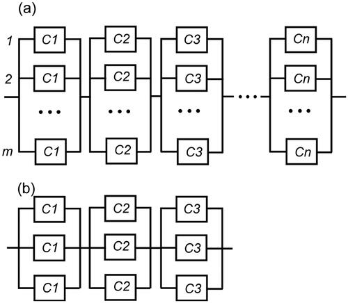
For $n=3$ sections with $m=3$ redundant components in each section (Figure 3b), inequality (12) becomes (18) $$(1-x_1^3)(1-x_2^3)(1-x_3^3)\le {(1-{[(x_1+x_2+x_3)/3]}^3)}^3={(1-{(p_f/p)}^3)}^3$$(18) where the left hand-side of (18) gives the actual reliability on demand of the system in Figure 3b and the right-hand side gives an estimate of the reliability on demand of the system in Figure 3b, calculated on the basis of the average probability of failure characterising the three varieties $C1,C2$ and $C3.$

For components of the same type but of three different varieties C1, C2 and C3, characterised by probabilities of failure 0.69, 0.14 and 0.04, the left-hand side of inequality (18) gives: $$R_{\mathit{\text{real}}}=(1-{0.69}^3)\times (1-{0.14}^3)\times (1-{0.04}^3)=0.67$$ for the real reliability on demand of the arrangement in Figure 3b.

If the reliability of the arrangement in Figure 3b is calculated on the basis of the average probability of failure $\overline{x}=p_f/p=261/900=0.29$ characterising the three varieties C1, C2 and C3, for the estimated system reliability on demand based on average probability of failure, the value: $$R_{\mathit{\text{est}}}={(1-{\overline{x}}^3)}^3={(1-{0.29}^3)}^3=0.93.$$ is obtained. The estimated value $R_{\mathit{\text{est}}}=0.93$ is 1.39 times greater than the real reliability on demand $R_{\mathit{\text{real}}}=0.67$ of the section.

2.3. Impact of variability on the system reliability predictions for parallel-series systems

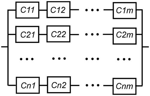
The system in Figure 4 includes $m\times n$ components of the same type and different variety. Monte-Carlo simulation experiments confirmed that no systematic overestimation or underestimation of the reliability on demand of the parallel series system in Figure 4 exists. This means that for certain combinations of reliability on demand values of the components, a prediction based on an average component reliability on demand leads to underestimation while for other combinations, the prediction leads to an overestimation of the system reliability on demand.

Figure 4. Reliability network of a parallel-series system with n parallel branches each including components from m varieties.

In conclusion, using average component reliabilities on demand to calculate system reliability on demand is not a dependable approach even for components working independently from one another, as it is fundamentally flawed. The extensive focus in reliability literature on predicting system reliability by using average component reliabilities cannot be justified because variability of the reliability on demand for components from the same type is always present.

Another key conclusion is that reducing the variability of components and reliability-critical parameters is crucial to the adequate estimation of system reliability.

Precision machining is an effective way to manufacture components to exact specifications, thereby reducing variability in their reliability-critical parameters. In addition, supplier quality management can ensure that components meet the required quality standards, with reduced variability of reliability-critical properties.

Conducting component testing is also essential in identifying potential variability issues and taking corrective action before the assembly process begins. Statistical process control techniques are an effective way to identify component variability and enable prompt corrective action to be taken. Implementing continuous monitoring and feedback along with statistical process control can ensure the quality and reliability of the produced components.

Removing sources of variability is another important technique for reducing component variability. It has been demonstrated in Todinov (2019) that to achieve the maximum reduction of variability, the sources of variation to be removed must be selected carefully, using a procedure based on the equation for the variance of a distribution mixture (Todinov, 2019).

3. Reducing variability of reliability-critical factors

3.1. Reducing variability by self-balancing

Self-balancing can also be used to reduce variability of reliability-critical parameters. Such are, for example, the gas turbines with a symmetric design that cancels out net axial forces by generating equal and opposite forces. This design cancels any variable forces because they always appear with the same magnitude and opposite directions. In addition, the symmetric design eliminates the need for axial bearings, as there is no net axial force to be supported. As a result, the number of components required is reduced, which also promotes higher reliability (Matthews, 1998).

Reducing the variability of loading in assemblies or systems by self-balancing can be found in rotating mechanisms (Meraz, 2005). In rotating machinery, unbalanced forces can cause significant stress and wear on the components, leading to increased maintenance costs and decreased reliability over time. By implementing self-balancing mechanisms, the machines are able to dynamically adjust for any imbalances, thereby reducing the amount of stress on individual components and increasing the overall reliability of the system. For example, modern gas turbines use self-balancing mechanisms such as tilting-pad journal bearings and active magnetic bearings to compensate for any imbalances caused by changes in operating conditions, such as changes in temperature and pressure. These self-balancing mechanisms allow the turbines to operate more efficiently and with less stress on individual components, resulting in increased reliability and decreased maintenance costs over the lifetime of the machine.

Another example of reducing variability by self-balancing is the use of active vibration control (AVC) systems. AVC systems utilise sensors and actuators to actively control the vibration and oscillations of various components and systems within an aircraft, such as engines, wings, and landing gear. By reducing these vibrations and oscillations, AVC systems can improve the reliability of the aircraft by reducing wear and mitigating the risk of fatigue failure or other forms of mechanical failure.

The use of active noise control (ANC) systems in industrial and transportation settings is a similar technique. ANC systems use sensors and actuators to actively cancel out unwanted noise and vibration, thereby improving the overall acoustic environment and reducing the risk of noise-induced stress in workers. These systems work by measuring the incoming noise or vibration and generating an opposite sound or vibration signal to cancel it out in real-time. For example, some heavy equipment used in construction and mining sites use ANC systems to actively cancel out the noise and vibration generated by engines and hydraulic systems. By reducing the amount of noise and vibration that reaches the operator, ANC systems can reduce the risk of noise-induced hearing loss. Additionally, ANC systems can improve the overall reliability of the equipment by reducing wear and fatigue caused by excessive vibration and noise.

Another example of improving reliability of assemblies or systems by self-balancing is the use of active balancing and monitoring circuits (Ciupitu, 2018; Ionescu & Drumea, 2019; Jeon et al., 2015; Kroics et al., 2016; Li et al.,2021; Zhen et al., 2017).

The Dynamic Variability Compensation System identifies real-time variability in mechanical performance and uses counteracting mechanisms to nullify these deviations. By pairing each variability with an opposing variability, the system creates a neutral state that enhances the overall mechanical reliability.

The first key component of the dynamic variability compensation system are the variability sensors. These measure mechanical inconsistencies or deviations, whether they are due to loading, wear, environmental factors, or any other influences.

The second key component are the compensation actuators. These are mechanisms designed to introduce an opposing variability or corrective measure.

The third key component is the predictive analysis unit. This is effectively a computing module that predicts future deviations based on past and current data.

The fourth key component is the control unit. It interprets sensor data, collaborates with the predictive analysis unit., and commands the compensation actuators.

Variability sensors constantly monitor the system, identifying any deviations or inconsistencies, in real-time. The control unit evaluates these deviations and, with the assistance of the predictive analysis unit, anticipates how they might evolve.

Once the nature and magnitude of a variability are identified, the control unit determines the necessary counteracting variability needed to neutralise it. Compensation actuators are then triggered to introduce this counteracting variability, effectively neutralising the initial deviation. By identifying and neutralising deviations in real-time, it offers a proactive approach to improving mechanical reliability, ensuring systems remain balanced and operate at their peak performance.

For example, if one part of a system is overloaded, asymmetric movement of a counterweight is activated so that the stresses appearing at a particular critical region are counterbalanced (Ciupitu, 2018; Zhen et al., 2017).

Potential applications can be found in manufacturing equipment. Machines requiring precision, like CNC machines, can benefit by ensuring each product is consistent despite machine wear or other influencing factors. Other potential applications are for robots working in dynamic environments, ensuring tasks are performed with low variability despite changing conditions.

The dynamic variability compensation system presents some limitations, one of which is the system complexity. Integrating multiple sensors, actuators, and computing modules complicate the design. This complexity leads to increased maintenance needs, increases the potential for more points of failure, and might require specialised training for personnel. Another limitation is the energy consumption. Constant monitoring and counteracting can increase the system’s power demands.

Self-balancing mechanisms often require additional components, such as counterweights or compensating masses. This can increase the overall weight and size of the system, which can be a disadvantage in applications where weight and size are crucial factors.

Introducing self-balancing features may lead to increased costs, both in terms of component manufacturing and system maintenance.

3.2. Reducing variability by promoting asymmetric response

3.2.1. Asymmetric response attained by inversion

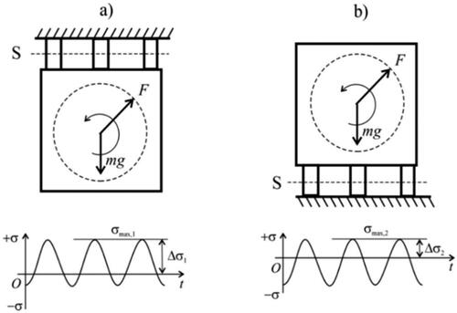
Countering variability of controlling factors and properties can be achieved not only by exploiting symmetrical arrangements and geometry. In certain cases, promoting asymmetric response may also reduce significantly the negative impact of variability and delay the occurrence of a failure mode. This concept is illustrated in Figure 5a, where the inversion of the electromotor’s position relative to its support introduces an asymmetric response related to the loading stress. In the original configuration (as shown in Figure 5a), most of the fluctuating loading stress is tensile, leading to a shorter fatigue life. However, when the position is inverted, most of the fluctuating loading stress becomes compressive, which enhances the fatigue life.

Figure 5. Inverting the relative position of an object with respect to its support delays a failure mode.

Another example of reducing variability by promoting asymmetric response through inversion can be seen in the enhancement of the reliability of a normally open mechanical switch soldered onto a printed circuit board (PCB), as shown in Figure 6a.

Figure 6. Enhancing the reliability of a mechanical switch by inversion from a normally open to a normally closed state.

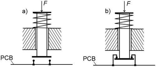
When variable force, denoted as F, is applied during the operation of the normally open switch in Figure 6a, the soldered points on the printed circuit board experience fluctuating stress with a relatively large magnitude. Over multiple operations, this fluctuating stress loading can lead to premature fatigue cracking. By obtaining asymmetric response through inversion, the normally open switch can be transformed into a normally closed one. This alters the activation process; instead of closing the normally open contacts, the activation now requires opening normally closed contacts. In the design depicted in Figure 6b, an excessive force F applied to the button does not translate into an excessive variable load on the soldered points. Due to this inversion, the severity of the fatigue loading on the soldered points is reduced dramatically and fatigue life is significantly enhanced.

3.2.2. Asymmetric response attained through nonlinear output

Asymmetric response countering variability can also be based on a on a non-linear output.

Systems with asymmetric response adjust the system’s behaviour based on its operating conditions, ensuring that the system remains reliable under increased variability of the controlling factors.

An example exploiting the asymmetry of the output characteristic to counter the negative effect of variability are the metal oxide varistors or Zener diodes (Horowitz & Hill, 1989). These devices are designed to conduct very little current below a certain voltage threshold and then conduct a large amount of current once the voltage exceeds that threshold.

Under normal voltage conditions, the Zener diode conducts very little current, essentially acting as an open circuit. The electronic device connected to the circuit operates normally.

If there is a sudden increase in voltage above the threshold level, the Zener diode becomes highly conductive almost instantly, diverting the excess current away from sensitive electronic components. This rapid change in conductivity at a specific voltage threshold protects other components in the system from experiencing damaging high voltage levels. Once the surge is over and the voltage drops below the threshold, the Zener diode returns to its high resistance state, ensuring that the normal operation of the device isn’t affected.

As a result, by leveraging the asymmetry of the V-I characteristic (essentially non-conductive below a certain voltage and highly conductive above it), the Zener diodes improve reliability. They ensure that electronic devices remain protected from transient voltage spikes that could otherwise damage or reduce the lifespan of the connected equipment.

3.3. Reducing variability during assembly operations

Assembly operations are sources of increased variability of reliability-controlling factors. When assembling loaded components, it is crucial to ensure that the assembly process does not add any additional stresses to the components. Imbalances can cause significant problems such as increased wear, decreased lifespan and even failure. To reduce the magnitude and variability of assembly stresses during assembling of loaded components, it is essential to use standardised assembly processes. For example, using standard precision alignment tools can greatly improve the level of balancing and reduce stresses. These tools, including laser alignment tools and dial indicators, can help ensure that components are properly aligned, which is crucial for reducing the variability of assembly stresses.

Employing controlled assembly processes to minimise variation is a powerful technique for reducing excessive assembly stresses. By implementing strict assembly instructions and quality control measures, variations in the assembly process can be minimised, leading to a reduction in assembly stresses. Thus, implementing standard torque specifications and tightening sequences is another effective technique for reducing the variability of assembly stresses. It is also essential to use high-quality fasteners with consistent properties to ensure that they are tightened evenly.

Controlled assembly process can also be implemented by automating certain assembly tasks which can help to reduce variability caused by human error and improve overall assembly reliability. In this respect, in order to improve consistency and accuracy during assembly, it is essential to use automation and robotics. Employing robots in assembly operations helps reduce variation and ensure that components are properly aligned.

Additionally, using special fixtures and tooling can make assembly easier and more accurate, further reducing variability. Support structures or jigs can provide additional stability and help ensure that components are properly aligned, leading to a reduction in assembly stresses.

Implementing static and dynamic balancing techniques during the assembly of rotating machinery is critical to reducing variability of stresses during operation. Balancing weights are often used to correct imbalances during assembly, and can be added or removed as necessary to achieve proper balance.

Designing products for assembly can help to reduce variability during assembly. Design modifications can be made to improve ease of assembly, further reducing variability of assemblies. For example, redesigning component interfaces can ensure that they fit together more smoothly, making assembly operations easier, thereby reducing variability.

Conclusions

1. The paper reveals a fundamental flaw in the existing approach for predicting system reliability on demand.

2. Using average component reliabilities on demand to calculate system reliability on demand is a fundamentally flawed approach even for components working independently from one another, as it is prone to significant errors.

3. The impact of assuming average component reliabilities on demand on the predicted reliability on demand of systems with independently working components logically arranged in series has been revealed by using a physical interpretation of the arithmetic mean-geometric mean algebraic inequality. The estimated system reliability based on average component reliability on demand is always greater than the actual reliability on demand of the system.

4. The impact of assuming average component reliabilities on the predicted reliability on demand of series-parallel systems has been revealed by using the physical interpretation of a novel algebraic inequality based on concave functions. The estimated system reliability on demand based on average component reliability on demand is always greater than the actual reliability of the system.

5. The impact of assuming average component reliabilities on the predicted probability of failure of systems with components logically arranged in parallel has been revealed by using a physical interpretation of the arithmetic mean – geometric mean algebraic inequality. The estimated probability of system failure on demand based on average component reliability on demand is always greater than the actual probability of failure on demand of the system.

6. It has been demonstrated that if there were no variability in the reliabilities of components of the same type, there would be no discrepancy between the estimated value for the system reliability on demand and the real value. The deviation of the reliability of components of the same type from the average value is inevitable, due to differences in age, operating conditions, environment, material and manufacturing flaws.

7. Useful domain-independent techniques have been introduced for countering the variability of safety-critical factors (i) by self-balancing, (ii) by promoting asymmetric response and (iv) through assembly operations.

Disclosure statement

No potential conflict of interest was reported by the author(s).

Additional information

Notes on contributors

Michael Todinov

Michael Todinov is a professor of mechanical engineering at Oxford Brookes University, UK. Prof. Todinov pioneered research on reliability analysis based on the cost of failure, repairable flow networks, domain-independent methods for reliability improvement and engineering optimisation and generating new knowledge by reverse engineering of algebraic inequalities.

References

- Aven, T. (2016). Risk assessment and risk management: Review of recent advances on their foundation. European Journal of Operational Research, 253(1), 1–13. https://doi.org/10.1016/j.ejor.2015.12.023
- Altshuller, G. S. (1984). Creativity as an exact science: The theory of the solution of inventive problems. Gordon and Breach Science Publishing.
- Altshuller, G. S. (1999). The innovation algorithm, TRIZ, systematic innovation and technical creativity. Technical Innovation Center, Inc.
- Budynas, R. G., & Nisbett, J. K. (2015). Shigley’s mechanical engineering design (10th ed.). McGraw-Hill.
- Budynas, R. G. (1999). Advanced strength and applied stress analysis (2nd ed.). McGraw‐Hill.
- Childs, P. R. N. (2014). Mechanical design engineering handbook. Elsevier.
- Ciupitu, L. (2018). Adaptive balancing of robots and mechatronic systems. Robotics, 7(4), 68. https://doi.org/10.3390/robotics7040068
- Collins, J. A. (2003). Mechanical design of machine elements and machines. John Wiley & Sons.
- Coria, I., Abasolo, M., Gutiérrez, A., & Aguirrebeitia, J. (2020). Achieving uniform thread load distribution in bolted joints using different pitch values. Mechanics & Industry, 21(6), 616. https://doi.org/10.1051/meca/2020090
- Dhillon, B. S. (2017). Engineering systems reliability, safety, and maintenance. CRC Press.
- Ebeling, C. E. (1997). Reliability and maintainability engineering. McGraw-Hill.
- French, M. (1999). Conceptual design for engineers (3rd ed.). Springer‐Verlag Ltd.
- Gere, J. M., & Timoshenko, S. P. (1999). Mechanics of materials. Stanley Thornes Publishers.
- Gullo, L. G., & Dixon, J. (2018). Design for safety. John Wiley & Sons.
- Hearn, E. J. (1985). Mechanics of materials (2nd ed., Vol. 1). Butterworth-Heinemann.
- Henley, E. J., & Kumamoto, H. (1981). Reliability engineering and risk assessment. Prentice‐Hall.
- Hoyland, A., & Rausand, M. (1994). System reliability theory. John Wiley and Sons.
- Horowitz, P., & Hill, W. (1989). The art of electronics. Cambridge University Press.
- Ionescu, C., & Drumea, A. (2019). Extended current range of active balancing and monitoring circuits for supercapacitor modules [Paper presentation]. 2019 IEEE 25th International Symposium for Design and Technology in Electronic Packaging (SIITME). https://doi.org/10.1109/SIITME47687.2019.8990782
- Jeon, S., Yun, J., & Bae1, S. (2015). Active cell balancing circuit for series connected battery cells [Paper presentation]. 9th International Conference on Power Electronics-ECCE Asia. June 1 - 5, 2015/63
- Kaplan, S., & Garrick, B. J. (1981). On the quantitative definition of risk. Risk Analysis, 1(1), 11–27. https://doi.org/10.1111/j.1539-6924.1981.tb01350.x
- Knowles, I. (1993). Is it time for a new approach? IEEE Transactions on Reliability, 42(1), 2–3.
- Kroics, K., Sokolovs, A., Sirmelis, U., & Grigans, L. (2016). Interleaved series input parallel output forward converter with simplified voltage balancing control [Paper presentation]. PCIM Europe 2016, 10 – 12 May 2016, Nuremberg, Germany.
- Li, H., Wang, J., Bai, G., & Hu, X. (2021). Research on self-balancing system of autonomous vehicles based on queuing theory. Sensors, 21(13), 4619. https://doi.org/10.3390/s21134619
- Lewis, E. E. (1966). Introduction to reliability engineering. John Wiley & Sons.
- Matthews, C. (1998). Case studies in engineering design. Arnold.
- MIL-STD-1629A. (1977). US Department of Defence procedure for performing a failure mode and effects analysis. US Department of Defence.
- Meraz, M. A., Yánez, A., Jiménez, C., & Pichardo, R. (2005). Self-balancing system for rotating mechanisms. Revista Facultad de Ingeniería - Universidad de Tarapacá, 13(2), 59–64.
- Modarres, M., Kaminskiy, M. P., & Krivtsov, V. (2016). Reliability engineering and risk analysis, a practical guide (3rd ed.). CRC Press.
- Mott, R. L., Vavrek, E. M., & Wang, J. (2018). Machine elements in mechanical design (6th ed.). Pearson Education.
- Norton, R. L. (2006). Machine design, an integrated approach (3rd ed.). Pearson International.
- Orloff, M. (2006). Inventive thinking through TRIZ (2nd ed.). Springer.
- O’Connor, P. D. T. (2002). Practical reliability engineering (4th ed.). John Wiley & Sons.
- Pahl, G., Beitz, W., Feldhusen, J., & Grote, K. H. (2007). Engineering design. Springer.
- Pao, P. S. (1996). Mechanisms of corrosion fatigue, book chapter. In ASM handbook (Vol. 19). Fatigue and Fracture.
- Pecht, M., Dasgupta, A., Barker, D., & Leonard, C. T. (1990). The reliability physics approach to failure prediction modelling. Quality and Reliability Engineering International, 6(4), 267–273. https://doi.org/10.1002/qre.4680060409
- Petroski, H. (1994). Design paradigms: Case histories of error and judgment in engineering. Cambridge: Cambridge University Press.
- Rantanen, K., & Domb, E. (2008). Simplified TRIZ (2nd ed.). Auerbach Publications.
- Ramakumar, R. (1993). Engineering reliability, fundamentals and applications. Prentice Hall.
- Samuel, A., & Weir, J. (1999). Introduction to engineering design: Modelling, synthesis and problem solving strategies. Elsevier.
- Steele, J. M. (2004). The Cauchy-Schwarz Master Class: An introduction to the art of mathematical inequalities. Cambridge University Press.
- Terninko, J., Zusman, A., & Zlotin, B. (1998). Systematic innovation: An introduction to TRIZ. CRC Press LLC.
- Todinov, M. T. (2023). Reliability-related interpretations of algebraic inequalities. IEEE Transactions on Reliability. Advance online publication. https://doi.org/10.1109/TR.2023.3236407
- Todinov, M. T. (2019). Methods for reliability improvement and risk reduction. Wiley.
- Todinov, M. T. (2002). Statistics of defects in one-dimensional components. Computational Materials Science, 24(4), 430–442. https://doi.org/10.1016/S0927-0256(01)00264-6
- Todinov, M. (2006). Equations and a fast algorithm for determining the probability of failure initiated by flaws. International Journal of Solids and Structures, 43(17), 5182–5195. https://doi.org/10.1016/j.ijsolstr.2005.09.007
- Thompson, G. (1999). Improving maintainability and reliability through design. Professional Engineering Publishing.
- Vose, D. (2000). Risk analysis, a quantitative guide (2nd ed.). John Wiley & Sons.
- Zhen, J., Ding, L., & Wang, X. (2017). Design of the smart pneumatic balance crane control system [Paper presentation]. 5th International Conference on Mechatronics, Materials, Chemistry and Computer Engineering (ICMMCCE 2017). https://doi.org/10.2991/icmmcce-17.2017.157