Modeling of landslides susceptibility prediction using deep belief networks with optimized learning rate control

Abstract

To overcome critical issues in landslide susceptibility modeling, a multifactor landslide susceptibility prediction model based on deep belief networks (DBN) with optimized learning rate control (LRC-DBN) was introduced in this study. The LRC-DBN model was applied to predict landslide susceptibility in Zhidan County, Shaanxi and its performance was compared against random forest, support vector machine and logistic regression models. The results show that the LRC-DBN model achieves a maximum AUC value of 0.941, which demonstrating higher predictive performance. The interpretability of LRC-DBN reveals that the development of loess landslides is more likely in areas with elevations ranging from 894.7 m to 998.5 m, slopes ranging from 49.6° to 64°, terrain undulations spanning 31.7 m to 91.0 m, rock type T₃y and terrain humidity ranging from 2.4 to 3.9. The result provides invaluable insights for local landslide prevention endeavors and can assist decision-making in urban planning.

Keywords:

• Landslide susceptibility
• deep learning
• conditional random field
• interpretability analysis

1. Introduction

Landslides, characterized by their wide distribution, high frequency and serious disaster losses, pose a grave threat to human life and property safety (Zhang et al. 2022). The Loess Plateau in China is a region of heightened landslide occurrence. Despite the modest overall population, its spatial distribution is concentrated and the terrain features steep slopes. Hence, the frequency of landslides has surged with increasing urbanization, presenting substantial challenges to livelihoods and productivity. Consequently, there is a pressing need to develop a landslide prediction methodology tailored to the unique characteristics of the Loess Plateau.

Landslide susceptibility prediction is crucial in landslide risk assessment and the precise positioning of potential landslide-prone areas (Som et al. 2023). Over recent decades, various methods leveraging GIS platforms have been employed for the landslide susceptibility prognosis. Among them, conventional statistical models have been extensively utilized, including heuristic models (Moragues et al. 2021), analytical hierarchy process models (Okalp and Akgün 2022) and mathematical-statistical models such as discriminant analysis (Pham et al. 2021), multiple linear regression (Balogun et al. 2021) and determinant coefficients (Li and Zhang 2017). However, these models are limited by their inability to reveal the nonlinear relationships between the various environmental factors in the landslide susceptibility modeling and often require substantial prior knowledge. Due to high accuracy and reduced dependence on prior knowledge (such as environmental factors to be normally distributed), machine learning has gained widespread use in landslide susceptibility prediction, with methods and models including artificial neural networks (Norsakinah et al. 2022, Gorsevski 2023), support vector machines (SVMs) (Zhao and Zhao 2021), decision trees (Gu et al. 2022), random forests (RFs) (Bien et al. 2023), multilayer perceptrons (Devara et al. 2021), logistic regression (LR) (Zhang et al. 2023) and stochastic gradient descent (Hong et al. 2020). Nonetheless, traditional machine learning approaches still encounter challenges in predicting landslide susceptibility: (1) representation learning requires extensive prior knowledge and assumption space and cannot fully capture the nonlinear relationships between environmental factors; (2) it is difficult to reduce errors in handling landslide and non-landslides samples; (3) the models are sensitive to data, such as missing values, noise and incorrect data; (4) the ‘black box’ nature of the models makes them lack interpretability of predicting landslides susceptibility values under the nonlinear coupling of various environmental factors. Therefore, it is necessary to explore a new machine-learning algorithm for predicting landslide susceptibility.

Deep learning, renowned for its formidable learning capabilities, broad scope and exceptional adaptability, stands out as a superior machine learning method with great advantages. Operating on a data-driven approach with minimal a priori knowledge and assumptions, deep learning offers a promising solution to overcome the limitations of traditional machine learning models and the application of deep learning models in landslide prediction. Nikoobakht et al. (2022) conducted a landslide susceptibility assessment in the northeastern region of Iran, employing a sophisticated 15-layer Convolutional Neural Network (CNN), which reveals that geomorphology, topographic parameters and hydrological conditions are pivotal factors in triggering landslides. In comparison to SVM, k-Nearest Neighbors (k-NN) and Decision Trees (DT), CNN demonstrates high accuracy with diminished computational errors. Azarafza et al. (2021) introduced an innovative Convolutional Neural Network with Deep Neural Network (CNN-DNN) for landslide susceptibility mapping. Their study found that, in contrast to various machine learning models, the CNN-DNN model exhibits better precision in the cartography of landslide susceptibility.

The aforementioned deep learning-based landslide susceptibility prediction mainly focuses on algorithm enhancements rather than improving the performance of landslide susceptibility modeling itself. Simple deep learning algorithm improvements often fall short in achieving the desired effect of landslide susceptibility prediction, specifically, in handling errors of the landslide and non-landslide samples (Ge et al. 2023). This sampling error seriously compromises the accuracy of the output variables of the deep learning model, consequently limiting the accuracy of the deep learning prediction of landslide susceptibility. Another critical concern in modeling landslide susceptibility is the lack of interpretability of the variables or features influencing the results, i.e. the interpretability of deep learning (Xiao et al. 2018). As deep learning models gain prevalence in critical environments for important predictions, the demand for transparency in machine learning is increasing. The risk lies in inappropriate, illegal decisions of the users or an inability to obtain detailed explanations of the purposes behind them. Whether in traditional machine learning or deep learning, both grapple with the challenge of fully explaining the mechanism behind the prediction of landslide susceptibility index under the influence of environmental factors. This issue is exacerbated by the ‘black box’ nature of most data-driven deep learning models.

Given this context, to surmount the challenges associated with deep learning in landslide prediction, efforts in this work are twofold: (1) to devise a method more applicable to the landslide susceptibility mapping in the Loess Plateau of China and (2) to address the dilemma posed by the ‘black box’ problem of deep learning models, further elucidating the relationship between each landslide feature and the corresponding predictive outcomes. Additionally, (3) this study seeks to determine whether, compared to conventional machine learning models, deep learning models exhibit stronger predictive accuracy. Building upon these, this article proposes a new deep learning algorithm, namely, the multifactor landslide susceptibility model (LRC-DBN) based on Deep Belief Networks (DBN). At the same time, three machine learning models- RF, LR and SVM are chosen for a comparative investigation. LRC-DBN is expected to analyze the correlations between various landslide points with higher accuracy, thus, extracting more features of environmental factors. Additionally, the article emphasizes the analysis of each environmental factor’s contribution to the decision of the prediction model and its connection to the prediction results, thereby deriving more interpretable conclusions. The research findings can offer novel perspectives on deep learning models in landslide prediction. Moreover, by explicating the intricate relationship between landslide factors and the occurrences, the study provides invaluable insights for local landslide prevention endeavors, where attention should be directed to anticipating specific factors. Concurrently, the susceptibility mapping outcomes at the county level can assist decision-making in the site selection of construction projects and urban planning.

2. The LRC-DBN model for landslide susceptibility prediction

2.1. The research methodology

Predicting the susceptibility of landslides is a complex nonlinear modeling problem, hence, satisfactory results may not be obtained using conventional statistical methods (Youssef et al. 2022). Traditional approaches in machine learning and data mining often rely on strong assumptions or substantial prior knowledge, facing various problems like errors occurring in handling landslide and non-landslide datasets in susceptibility modeling. In this article, a new deep learning model, LRC-DBN, is proposed to address these issues and apply it for the first time to a real-world landslide prediction dataset. The algorithm flow (Figure 1(a)) is outlined as follows:

Figure 1. Algorithm flow and Dropout architecture: (a) algorithm flow; (b) dropout architecture.

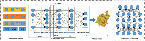
1. Analysis and screening of landslide factors: leveraging landslide record information and basic environmental factors, the frequency ratio method is employed to calculate the frequency ratio of each basic environmental factor.

2. Establishment of spatial dataset: the processed frequency ratio values serve as input variables to construct a spatial dataset of landslides and non-landslides for the model. The dataset is then divided into a training set and a test set for the model development.

3. Training and simulation of DBN: Using the spatial dataset of landslides and non-landslides as input variables, training and simulation are conducted within the DBN neural architecture.

4. Modeling of LRC-DBN: starting from the lower layers to the upper levels, unsupervised and voracious optimization algorithms are employed for parameter initialization. Subsequently, the BP algorithm refined the LRC-DBN, accomplishing nonlinear classification optimization through the Softmax classifier, with regularization processing based on the Dropout technique.

5. Model performance evaluation: the performance of model is assessed by metrics such as false negatives, false positives, true negatives and true positives. The ROC curve is employed to further evaluate the performance.

2.2. Landslide susceptibility model

2.2.1. Pre-training of LRC-DBN

In the pre-training phase, a greedy unsupervised optimization algorithm was utilized, progressing through lower to higher layers and initializing all parameters (Li et al. 2022). Within the conventional DBN architecture, multiple RBMs were integrated. In this study, each RBM comprises two layers of neurons: the visible layer, fed with historical landslide disaster training data; and the hidden layer, responsible for feature extraction. The DBN is constructed by stacking multiple RBMs together.

Within the RBM framework, the probability distribution of weights and biases for each unit in different layers is defined by an energy function, expressed as: $$E\left(v,h\theta \right)=-a^{T}v-b^{T}h-v^T\mathit{\text{Wh}}$$ (1) $$=-\sum _{i=1}^n{a}_i{v}_i-\sum _{i=1}^n{a}_i{v}_i-\sum _{j=1}^n{b}_j{h}_j-\sum _{i=1}^n\sum _{j=1}^n{v}_j{W}_{\mathit{\text{ij}}}{h}_j$$(1) where $\theta =\left\{w_{\mathit{\text{ij}}},a_i,b_j\right\}$ represents the parameters that need optimization, exerting a significant influence on the algorithm’s performance. n is the number of units in the visible layer, m is the number of units in the hidden layer, w_ij denotes the connection weight between visible unit I and hidden unit j and a_j and b_j denote the biases of visible unit i and hidden unit j, respectively. Based on these parameters, the joint probability distribution of (v, h) can be obtained. (2) $$P\left(v,h\right|\theta )=\frac{\mathrm{\text{exp}}(-E(v,h\theta \left)\right)}{\sum _{v,h}\mathrm{\text{exp}}(-E(v,h\theta \left)\right)}$$(2)

To obtain the marginal distribution of P(v,h), the probability assigned by the RBM model to the visible nodes is computed using the formula: (3) $$P\left(v,|\theta \right)=\frac{\sum _h\mathrm{\text{exp}}(-E(v,h\theta \left)\right)}{\sum _{v,h}\mathrm{\text{exp}}(-E(v,h\theta \left)\right)}$$(3)

Concerning the parameter $\theta ,$ it can be obtained through maximizing the log-likelihood function of RBM on the training samples.

Here, C represents the total number of training samples, and c is the label of the training sample. The purpose of employing RBM is to derive the optimal $\theta ,$ even as $\mathrm{\text{ln}}P\left(v^c\right|\theta )$ is maximized. To achieve this, let $L(\theta )=\mathrm{\text{ln}}P\left(v^c\right|\theta )$ and employ stochastic gradient descent to find the maximum value of $L(\theta ),$ thereby obtaining the optimal ${\theta }^{*}$ by computing partial derivatives for each parameter. (4) $$\{\begin{array}{l}\frac{\partial L\left(\theta \right)}{\partial w_{\mathit{\text{ij}}}}=\epsilon \left\{{\left(v_i{h}_j\right)}_{\mathrm{\text{data}}}-{\left(v_i{h}_j\right)}_{\mathrm{\text{model}}}\right\}\\ \frac{\partial L\left(\theta \right)}{\partial a_i}=\epsilon \left\{{\left(v_i\right)}_{\mathrm{\text{data}}}-{\left(v_i\right)}_{\mathrm{\text{model}}}\right\}\\ \frac{\partial L\left(\theta \right)}{\partial b_j}=\epsilon \left\{{\left(h_j\right)}_{\mathrm{\text{data}}}-{\left(h_j\right)}_{\mathrm{\text{model}}}\right\}\end{array}$$(4)

Here, $\epsilon$ represents the learning rate, while ${(\bullet )}_{\mathrm{\text{data}}}$ and ${(\bullet )}_{\mathrm{\text{model}}}$ denote the mathematical expectations of the distribution determined by the model and the mathematical expectations on the training dataset, respectively.

This study employs contrastive divergence for computation. However, when utilizing the CD algorithm, employing a fixed learning rate may lead to difficulties in convergence or the emergence of local optima. To address this issue, with the momentum learning rate incorporated, a momentum term in the parameter update process is introduced, as expressed in the following formula. (5) $$\{\begin{array}{l}\Delta w_{\mathit{\text{ij}}}^n=\epsilon \frac{\partial L\left(\theta \right)}{\partial w_{\mathit{\text{ij}}}^n}+\rho \Delta w_{\mathit{\text{ij}}}^{n-1}\\ \Delta a_i^n=\epsilon \frac{\partial L\left(\theta \right)}{\partial a_i^n}+\rho \Delta a_i^{n-1}\\ \Delta b_j^n=\epsilon \frac{\partial L\left(\theta \right)}{\partial b_j^n}+\rho \Delta b_j^{n-1}\end{array}$$(5) where n denotes the number of iterations for each layer of RBM, represents the momentum learning rate, and $\rho$ falls within the interval [0,1). The incorporation of the momentum learning rate ensures that the direction of each parameter update is determined not only by the gradient direction of the likelihood function under the current sample but also by the current gradient direction, thus enhancing the accuracy of the entire algorithm and providing a more precise reflection of the relationships between various influencing factors causing landslides.

2.2.2. Fine-tuning of LRC-DBN

Following the pre-training phase, the BP algorithm was employed to fine-tune LRC-DBN, aiming to enhance its predictive performance (Dou et al. 2020). The initial parameters obtained for each RBM are adjusted and trained to optimize the network parameters at each layer.

2.2.3. LRC-DBN nonlinear classification optimization

Given the diverse and intricate nonlinear relationships among landslide factors, the Softmax regression is employed to address the nonlinear multiclassification issue in the predictive model of this article. The approach involves integrating the Softmax classifier into the top layer of the enhanced DBN. Assuming the Softmax regression model has k training sample sets denoted as $\left\{\left(x^1,y^1\right),\dots ,\left(x^k,y^k\right)\right\},$ the hypothesis function of Softmax regression can be expressed as follows: (6) $$h_{\theta }\left(x^i\right)=\{\begin{array}{c}\Delta w_{\mathit{\text{ij}}}^n=\epsilon \frac{\partial L\left(\theta \right)}{\partial w_{\mathit{\text{ij}}}^n}+\rho \Delta w_{\mathit{\text{ij}}}^{n-1}\\ \Delta a_i^n=\epsilon \frac{\partial L\left(\theta \right)}{\partial a_i^n}+\rho \Delta a_i^{n-1}\\ \Delta b_j^n=\epsilon \frac{\partial L\left(\theta \right)}{\partial b_j^n}+\rho \Delta b_j^{n-1}\end{array}=\frac{1}{\sum _{j=1}^k\mathrm{\text{exp}}\hspace{0.17em}\left({\theta }_j^T{x}^i\right)}\{\begin{array}{c}\mathrm{\text{exp}}\hspace{0.17em}\left({\theta }_1^T{x}^i\right)\\ ⋮\\ \mathrm{\text{exp}}\hspace{0.17em}\left({\theta }_k^T{x}^i\right)\end{array}$$(6) here, $h_{\theta }\left(x^i\right)$ computes the probability value $P\left(y^i=j\right|x^i;\theta )$ for the test sample xⁱ belonging to category j, where θ represents the model’s parameter vector. The cost function can be delineated as: (7) $$J\left(\theta \right)=-\frac{1}{k}\left[\sum _{i=1}^k\sum _{j=1}^{t}I\{y^i=j\}\mathrm{\text{log}}\frac{\mathrm{\text{exp}}\hspace{0.17em}\left({\theta }_j^T{x}^i\right)}{\sum _{j=1}^t\mathrm{\text{exp}}\hspace{0.17em}\left({\theta }_j^T{x}^i\right)}\right]$$(7)

In this equation, t signifies the number of classifications, with landslides categorized into four classes (t = 4). The indicator function I{·} takes the value 1 when the condition inside the braces is true, and 0 otherwise.

2.2.4. Regularization of LRC-DBN

To improve precision and mitigate overfitting, this study employs Dropout for regularization. During the pre-training phase, while keeping the neural network input and output unchanged, a specific probability for Dropout is applied to randomly select the weights of hidden layer nodes, with the initial probability of 50%. With each adjustment, a portion of neurons does not participate in the forward propagation training process.

2.3. Evaluation of landslide susceptibility mapping

2.3.1. Evaluation of the accuracy of statistical indicators

This study employs several statistical indicators, namely Positive Prediction Rate (PPR), Negative Prediction Rate (NPR) and Total Accuracy (TA), to assess the predictive performance of different models (Park et al. 2019). PPR calculates the proportion of predicted positive cases among all positive cases, while NPR calculates the proportion of predicted negative cases among all negative cases. The two indicators can evaluate the prediction ability of the landslide susceptibility model for landslides and non-landslides samples, respectively (Youssef et al. 2022). TA is used to assess the prediction accuracy of all test datasets. The calculations for these statistical indicators are as follows: (8) $$\mathrm{\text{TA}}=\frac{\mathrm{\text{TP}}+\mathrm{\text{TN}}}{\mathrm{\text{TP}}+\mathrm{\text{TN}}+\mathrm{\text{FP}}+\mathrm{\text{FN}}}$$(8) where True Positive (TP) represents the number of correctly classified landslide grids; True Negative (TN) represents the number of correctly classified non-landslide grids; False Positive (FP) represents the number of incorrectly classified landslide grids, i.e. non-landslide grids incorrectly classified as landslide grids; False Negative (FN) represents the number of incorrectly classified non-landslide grids, i.e. landslide grids incorrectly classified as non-landslide grids. TA represents the overall prediction accuracy of the model, with the larger TA indicating better accuracy in landslide susceptibility prediction (Lima et al. 2023).

2.3.2. Evaluation based on ROC curve

The Receiver Operating Characteristic Curve (ROC) finds widespread application in evaluating the performance of landslide susceptibility models, reflecting the relationship between specificity (False Positive Rate [FPR]) and sensitivity (True Positive Rate [TPR])(Dahal and Lombardo 2023). Specificity and sensitivity are calculated using the following formulas: (9) $$\mathrm{\text{FPR}}=\frac{\mathrm{\text{FP}}}{\mathrm{\text{FP}}+\mathrm{\text{TN}}}$$(9) (10) $$\mathrm{\text{TPR}}=\frac{\mathrm{\text{TP}}}{\mathrm{\text{TP}}+\mathrm{\text{FN}}}$$(10)

Presenting a ROC curve graphically, specificity serves as the x-axis and sensitivity as the y-axis. Generally, the ROC curve is above the y = x line, so the area under the curve (AUC) of the ROC curve usually falls in the range [0.5, 1]. The closer the ROC curve is to the top left corner, the larger the AUC is, signifying better performance in the landslide susceptibility prediction model (Sun et al. 2023).

2.3.3. Interpretability of deep learning in landslide susceptibility prediction

In recent years, deep learning has demonstrated significant advancements across various research fields. However, its credibility is often hindered by the lack of interpretability, which refers to providing understandable explanations to humans (Dimililer et al. 2021). Such ability can be categorized into intrinsic interpretability and post hoc interpretability.

Intrinsic interpretability, also known as pre hoc interpretability, refers to the interpretability embedded within the model before the network is trained. This is predominantly utilized in simpler network models. It is a common practice to directly use interpretable models or implement the intrinsic interpretability of network models (Grabowski et al. 2022). Post hoc interpretability aims to extract information from a trained model, making it particularly relevant for complex network models. Moreover, it can be further divided into global interpretability and local interpretability. Global interpretability involves explaining and comprehending the model’s decision based on the feature space and overall model structure of the entire dataset, corresponding to global interpretability methods, which are typically interpreted at the model level. Local interpretability focuses on explaining the model’s decision by analyzing changes in each dimension of the input sample’s features and their effect on the output result, corresponding to local interpretability methods, which are usually interpreted at the data level (Chiang et al. 2022). In this study, both local and global interpretations of the extended county landslide spatial dataset were conducted based on the prediction distribution map and integral gradient.

3. Description of the study area and landslide inventory

3.1. The study area

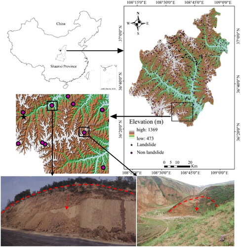
Zhidan County, situated in the loess hilly and gully region in the northwest of Yan’an City, Shaanxi Province, spans geographical coordinates from 108° 11'56 ″ E to 109° 3'48 ″ E and 36° 21'23 ″ N to 37° 11'47 ″ N (Figure 2). The county stretches approximately 70 km from east to west, and 92.56 km from south to north, covering a total area of about 3781 km2. Zhidan County experiences a typical temperate continental monsoon climate, with an annual average temperature of 8.1 °C, a minimum temperature of −28 °C and a maximum temperature of 37.4 °C. Being located in the Loess Plateau, the County witnesses sparse rainfall, with an annual average precipitation of approximately 472.2 mm. Rainfall is unevenly distributed throughout the year, concentrating in June and August with about 292.9 mm. Rainfall mainly occurs in the form of rainstorms, constituting 56% of the annual rainfall. The rainfall distribution is uneven and exhibits a gradual increase from the northwest to the southeast, decreasing towards the north. Zhidan County’s lithology comprises Triassic clastic sedimentary rocks (T₂t, T₂w), Pliocene Sanzhima red soil (T₃h, T₃y) and Quaternary system (Qp_1-3). Figure 2 illustrates the general situation of landslides in this area. As can be seen, there are 289 existing landslides, mainly small shallow overburden landslides with mostly small and medium-sized volumes (Government 2023).

Figure 2. Landslide inventory map of study area.

3.2. Analysis of landslide environmental factors

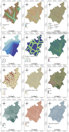
Data sources for this study include (1) landslide catalog information and field survey data obtained from the Land and Resources Department at the County level; (2) 30 m resolution DEM data; (3) 1:10,000 scale Zhidan County rock type distribution map; (4) 30 m resolution Landsat TM8 remote sensing images, etc. Considering field conditions and the environmental factors influencing landslides development, and drawing insights from existing literature, the final selection of input variables for the susceptibility model included elevation, slope, aspect, mean annual precipitation (MAP), distance to road, topographic roughness, total surface radiation, lithology, Topographic Wetness Index (TWI), Normalized Difference Building Index (NDBI), Normalized Difference Vegetation Index (NDVI), Modified Normalized Difference Water Index (MNDWI), amounting to a total of 12 variables (Figure 3).

Figure 3. Environmental factors for landslides. (a) DEM, (b) Slope, (c) aspect, (d) MAP, (e) distance to road, (f) topographic roughness, (g) lithology, (h) TWI, (i) NDVI, (j) NDBI, (k) MNDWI, (l) total surface radiation.

4. Results of landslide susceptibility modeling

4.1. Landslide spatial dataset

This study utilized 12 environmental factors obtained as input variables for deep learning. The landslide dataset incorporates a total of 202 landslide occurrences spanning the years 2013 to 2023. These instances were compiled from historical records, field surveys and remote sensing interpretations. Additionally, these instances were randomly generated in regions with a slope less than 2°. The transformation of both landslide and non-landslide points into polygons, followed by rasterization, resulted in a dataset of 9754 grid cells, including 4877 landslide grid cells converted from landslide areas and 4877 non-landslide grid cells randomly selected from non-landslide areas. These grids were randomly divided and merged in a 70/30% ratio to form the training and test sets (Tingyu et al. 2019). Subsequently, the LRC-DBN model was employed to predict the landslide susceptibility in Zhidan County using these datasets and was compared with LR, RF and SVM models.

4.2. The results of landslide susceptibility mapping in the study area

4.2.1. The result derived from the LRC-DBN model

The proposed LRC-DBN model in this study effectively circumvents the predicaments related to difficult convergence or local optima during the training phase. The model employs Dropout to mitigate the issue of overfitting and introduces Softmax regression for nonlinear classification optimization. The model’s parameter configurations are detailed in Table 1.

Table 1. Parameters of LRC model.

Parameter	Values
Number of input features	12
Number of output features	5
Number of iterations	400
Dropout	0.5
Learning rate $\epsilon$	1
Initial value of the momentum learning rate $\rho$	0.5

Furthermore, in the present work, based on the training samples, the layers of the Restricted Boltzmann Machine (RBM) were progressively increased from one to eight layers, with corresponding adjustments to the node count within each layer of the RBM. The achieved accuracy results are presented in Table 2.

Table 2. Prediction experimental results of changing the number of RBM layers and nodes.

Number of RBM layers	Number of nodes in each RBM layer	Accuracy (%)
1	20	78.82
2	20, 40	82.61
3	20, 40, 40	87.39
4	20, 40, 40, 80	90.82
5	20, 40, 40, 80, 40	92.57
6	20, 40, 40, 80, 40, 20	92.76
7	20, 40, 40, 80, 40, 20, 20	92.84
8	20, 40, 40, 80, 40, 20, 20, 20	92.93

The results indicate that as both the quantity of layers and nodes in the RBM increase, the predictive accuracy rises proportionately. Once the RBM layers reach 5, the predictive accuracy stabilizes at 92.5%, demonstrating stability and precision in predictions.

The trained LRC-DBN model is applied to predict the landslide susceptibility for the entire study area in Zhidan County, contributing to the final landslide susceptibility mapping (LSM). In addition, using the natural breakpoint classification method, Zhidan County is categorized into five levels: extremely high, high, medium, low and extremely low, with corresponding area ratios of 14.51%, 11.25%, 12.97%, 18.91% and 42.36%, respectively (Figure 4(a)).

Figure 4. Landslide susceptibility maps: (a) LRC-DBN, (b) RF, (c) LR, (d) SVM.

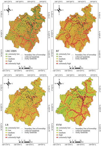
4.2.2. Results from the RF model

RF is a tree-based classifier and is a commonly used model for predicting the susceptibility of landslides. The accuracy of RF mainly depends on parameters such as the number of factor features (m) and the number of trees (t). In predicting landslide susceptibility for Zhidan County, the parameters m and t are set to 3 and 800, respectively, using the out-of-bag error method. The RF model is also used to predict the landslide susceptibility for the entire study area before resulting in an LSM. The predicted area ratios for extremely high, high, medium, low and extremely low landslide susceptibility areas are 11.08%, 15.48%, 20.17%, 26.24% and 27.03%, respectively (Figure 4(b)).

4.2.3. The result derived from LR and SVM models

The LR model is characterized by a linear regression model equation and a Sigmoid function. It essentially assumes that the data follows a certain distribution, followed by maximum likelihood estimation to estimate the parameters. LR is simple and efficient in implementation, showing qualities like easy explanation, fast calculation and easy parallelism. When modeling LR, the L2 regularization term is set to enhance the anti-disturbance ability, the penalty coefficient (C) is set to 0.5 and the stop standard is set to 10⁻⁴. The predicted area ratios of extremely high, high, medium, low and extremely low landslide susceptibility areas are 10.38%, 15.22%, 23.45%, 24.93% and 26.02%, respectively (Figure 4(c)).

For the SVM model, the penalty coefficient (C) is set to 1.0 and the radial basis kernel function with the coefficient γ set to 0.3 is used. The predicted area ratios of extremely high, high, medium, low and extremely low landslide susceptibility areas are 15.25%, 17.33%, 17.94%, 21.62% and 27.86% (Figure 4(d)). Statistical results of landslide susceptibility prediction are detailed in Table 3.

Table 3. Statistical results of landslide susceptibility prediction.

Models	Area ratio (%)
	Extremely high	High	Medium	Low	Extremely low
LRC-DBN	14.51	11.25	12.97	18.91	42.36
RF	11.08	15.48	20.17	26.24	27.03
LR	10.38	15.22	23.45	24.93	26.02
SVM	15.25	17.33	17.94	21.62	27.86

According to the statistical outcomes derived from the LSMs generated by the four models. The SVM model predicts the highest proportion in the extremely susceptible areas, with a prevalence of 27.86% in the extremely low susceptibility areas. Conversely, the LRC-DBN model predicts the extremely low susceptibility areas at 42.36%, while its proportion in the extremely high susceptible areas stands at 14.51%. This suggests that the LRC-DBN model excels in delineating non-landslide areas during landslide prediction, providing clear classification results and maintaining predictive prowess for landslide susceptibility areas within this framework.

4.3. Evaluation of landslide susceptibility mapping

4.3.1. Accuracy of statistical indicators

Table 4 presents the statistical measurement results for each landslide prediction model. Notably, the LRC-DBN shows better prediction performance than other traditional machine learning models and deep learning models in terms of negative prediction rate, positive prediction rate and overall prediction rate. The self-screening method effectively eliminates incorrect samples, providing high-quality data for model learning. The application of Dropout enables the capturing of deeper interactive relationships between environmental factors, making the LRC-DBN distinguish itself from other machine learning models.

Table 4. Landslide prediction performance.

Models	LRC-DBN	RF	SVM	LR
TP	1067	1029	985	947
TN	1073	989	945	940
FP	389	475	517	522
FN	397	433	479	517
PPR (%)	86.14	78.14	74.12	72.73
NPR (%)	85.33	80.34	75.79	72.93
TA (%)	84.28	79.19	74.92	72.83

4.3.2. ROC curve

The ROC curve evaluates the model performance through hit rate and false alarm rate, with AUC representing the area under the ROC curve. The curve primarily serves to measure the model’s generalization performance. Figure 5 illustrates that LRC-DBN exhibits better performance than other models in terms of precision and recall. This suggests that LRC-DBN not only overcomes the limitations of other models but significantly enhances the model’s nonlinear expression ability through the incorporation of Dropout.

Figure 5. ROC curves for each landslide susceptibility prediction model.

5. Discussion

5.1. Analysis of LRC-DBN model

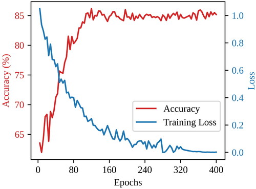
As iterations progress, the fluctuation curves of the training loss and test accuracy in the training datasets for LRC-DBN are illustrated in Figure 6. Figure 6 indicates a rapid drop of the loss value from 1.1 to 0.2 within the initial 150 iterations, which initially declines and eventually stabilizes. Simultaneously, the accuracy swiftly rises from 0.62 to 0.85, gradually stabilizing and reaching the peak. This indicates a prompt convergence and consistent performance, rendering the LRC-DBN model reasonably involved.

Figure 6. Loss and accuracy curves with number of iterations.

The mapping results of landslide susceptibility highlight the superior performance of the LRC-DBN model compared to traditional models such as RF, LR and SVM. Several advantages contribute to this exceptional performance. For instance, the model employs the Dropout to address biases arising from factors like man-made annotation errors and data collection inaccuracies; during the pre-training phase, it utilizes momentum learning rates to prevent algorithm convergence difficulties or premature local convergence. LRC-DBN can fully leverage the input data to learn nonlinear relationships among complex environmental factors, demonstrating strong feature extraction capabilities and excellent interpretability. However, despite its advantages, the LRC-DBN is relatively complicated compared to other deep learning and machine learning models. Therefore, future improvements will focus on simplifying and optimizing the model to the best without sacrificing accuracy.

5.2. Interpretability of LRC-DBN model in landslide susceptibility mapping

The interpretation of the deep learning model’s results for predicting landslide susceptibility involves examining the impact of single factors, the interaction of dual factors and the contribution of landslide environmental factors.

5.2.1. Single factors

The interpretation of environmental single-factor predictions involves inputting the landslide samples into the model, thus, deriving the probability of landslide susceptibility. The statistical distribution chart of environmental single factors reveals the impact of different single factors on the prediction results of landslide susceptibility from the perspective of natural causation. Analyzing 2926 samples in the test set provides the distribution of each environmental factor in different intervals. Taking slope as an example, the prediction distribution is obtained by statistical analysis of each sample according to the distribution of slopes, as illustrated in Tables 5 and 6. Q2 represents the second quartile of the probability in each slope range.

Table 5. One-way interpretable results for landslide susceptibility prediction based on slope.

		Number of landslides	Q2
Slope intervals (°)	[0–11.2]	284	0.071
	[11.2–16.4]	365	0.071
	[16.4–19.1]	467	0.334
	[19.1–24.7]	506	0.591
	[24.7–27.5], [49.6–64)	578	0.713
	[27.5–49.6]	726	0.902

Table 6. One-way interpretable results for landslide susceptibility prediction based on distance to road.

		Number of landslides	Q2
Distance to road intervals (m)	[0–500]	558	0.071
	[500 − 1000]	495	0.470
	[1000 − 1500]	386	0.397
	[1500 − 2000]	118	0.484
	[2000 − 10,000)	3	0.543

In Table 5, the slope ranging from 0° to 11.2° and 11.2° to 16.4°Contribute to a relatively small part of the samples (284 and 365 cases), accounting for about 9.7% and 12.4% of the total, respectively. The largest number of samples (726 cases, around 24.8% of the total) falls within 27.5°−49.6°. The slopes in 0°−16.4°display a very low probability of landslides, all less than 0.2 and Q2 in both intervals is 0.071. The probability of landslides with slopes of 19.1°−24.7° and 49.6°−64° is concentrated between 0.7 and 0.8, with Q2 at 0.713. For slopes within 27.5°−49.6°, the probability of landslides is mainly between 0.9 and 1, with Q2 at 0.902, indicating a high probability of landslides. As an important environmental factor in susceptibility assessment, slope size directly affects the occurrence of landslides. Within the 0°−49.6° slope range, the probability of landslides in the study area increases with increasing slope size, while in the 49.6°−64° range, the probability of landslides decreases compared to that in the 24.7°−27.5° range. This is because smaller slopes are generally more stable, while larger slopes are generally less prone to collapse due to less accumulation of weathering layers, less human activity and better drainage.

Conversely, Table 6 reveals a scarcity of data in the 2000 − 10,000 range (76 cases, ∼2.59% of the total) and the 1500 − 2000 range (84 cases, ∼2.87% of the total). As the distance to the road decreases, there is a higher probability of landslides. In the 500 − 1000 range, more than half of the samples showed landslide susceptibility probabilities between 0 and 0.5, with Q2 at 0.563, whereas in the 0–500 range, more than half of the samples displayed probabilities between 0.5 and 0.9, with Q2 at 0.617. Road construction usually requires land development and renovation, including cutting and filling, which damage the original terrain and soil structure, heightening the risk of landslides. Additionally, road building alters surface runoff patterns, leading to concentrated water flow and increasing the likelihood of soil erosion, further weakening the stability of the soil and ultimately increasing the risk of landslides.

5.2.2. The interaction of dual factors

Regarding single-factor statistics, a more comprehensive examination of the interaction of two factors was carried out, focusing on the results with high correlation (Bui et al. 2020). Taking DEM and Slope as an example, the statistical results of Altitude and Slope were obtained, and the statistical relationship of Altitude and Slope is presented in Table 7.

Table 7. Interpretable result of interaction between altitude and slope.

Probability of landslide occurrence		Altitude intervals (m)
		[397–794.6]	[794.6–803.9], [1293.2 − 1421)	[803.9–829.7], [1107.1 − 1293.2]	[829.7–845.2], [1033.6 − 1107.1]	[845.2–894.7], [998.5 − 1033.6]	[894.7–998.5)
Slope intervals (°)	[49.6–64)	0.175	0.481	0.475	0.693	0.778	0.913
	[24.7–27.5], [27.5–49.6]	0.181	0.4	0.429	0.634	0.652	0.862
	[16.4–19.1], [19.1–24.7]	0.158	0.272	0.306	0.525	0.475	0.758
	[11.2–16.4]	0.112	0.127	0.124	0.264	0.28	0.493
	[0–11.2]	0.102	0.102	0.102	0.114	0.122	0.253
	[24.7–27.5]	0.104	0.104	0.104	0.104	0.105	0.185

Table 7 delineates that, when the slope is between 0° and 16.4°, the material accumulation demonstrates a robust resistance, outweighing the propensity to collapse, resulting in the absence of landslides. With a constant elevation, the landslide susceptibility probability initially increases and then decreases with the increasing slope, peaking between 27.5° and 49.6°. Similarly, under the same slope, the landslide susceptibility probability initially increases, and then, decreases with the increase of elevation, peaking between 894.7 m and 998.5 m. Notably, at elevations of 894.7 m and 998.5 m, the landslide susceptibility probability of slope in the range of 49.6° to 64° attains the highest value (0.913). This indicates that the elevation of 894.7 m to 998.5 m facilitates material accumulation and landslide development, conducive to the deposition of some slope and alluvial deposits. Following rock weathering, the accumulated material can be easily transported from the 979.4 m to 1369.8 m area to the 894.7 m to 998.5 m area via slope processes. During the process, encountering a slope of 19.1° to 64° significantly increases the likelihood of the deposited accumulation evolving into landslides.

As shown in Table 8, with constant terrain roughness of 19.7 to 91 m, the probability of landslide susceptibility initially increases followed by a decrease with increasing terrain moisture. At a terrain roughness of 28.3 m to 91 m and a TWI of 2.4 to 3.9, the average landslide susceptibility probability (0.892) is the highest. In areas with high terrain moisture, the accumulation layer on the slope, featuring high water content and low shear strength of the slope body, is prone to developing into landslides under suitable terrain roughness. However, excessively high terrain moisture, often associated with well-developed water systems, facilitates erosion and transportation of slope materials, rendering conditions unfavorable for landslides.

Table 8. Interpretable result of interaction between topographic roughness and TWI.

Probability of landslide occurrence		Topographic roughness intervals (m)
		[0–12.5]	[12.5–19.7]	[19.7–24.6]	[24.6–28.3]	[28.3–31.7]	[31.7–91]
TWI intervals	[2.4–3.9]	0.195	0.24	0.398	0.533	0.634	0.892
	[3.9–5.2], [5.2–6.9]	0.183	0.267	0.362	0.561	0.658	0.785
	[6.9–10.4], [10.4–27.1)	0.164	0.199	0.265	0.434	0.458	0.562

5.2.3. The contribution of landslide environment factors

This study assessed the contribution of each slope environmental factor to the decision process of the LRC-DBN model by integrating the gradients of each sample concerning the slope environmental factors and computing the expected value. To simplify the calculation, the baseline was set to 0 and the approximate method employed 50 steps. The results derived from the sum of the contributions of the slope environmental factors, calculated based on the integral gradient, revealed the following key insights: (1) the contribution of landform and geology to the slope was relatively large, approximately 0.31 and 0.18, respectively. (2) Surface cover and hydrological environment exhibited relatively minor contributions to the slope, about −0.03 and 0.02, respectively. (3) Slope, lithology and elevation exerted a significant impact on the slope, contributing about 0.14, 0.12 and 0.08, respectively, aligning with previous findings. (4) NDVI made a negative contribution (around −0.04), MNDWI's contribution was nearly 0 and NDBI's contribution was less than 0.01. These results indicate that NDVI, MNDWI and NDBI are not the dominant factors causing landslides in Zhidan County. In conclusion, the landslides in Zhidan County featured by the loess plateau landform are significantly influenced by factors including slope, lithology, elevation, slope orientation and topographic roughness.

6. Conclusion

This study introduced a multifactor-focused deep learning model (LRC-DBN) based on Deep Belief Networks (DBN) with optimized learning rate control for landslide susceptibility prediction mapping. Compared with machine learning models such as RF, SVM and LR, the proposed model demonstrates many advantages, achieving the highest AUC value of 0.941 and better modeling results than other models. By integrating the inherent mechanisms of landslides and the interpretability of deep learning networks, LRC-DBN transcends the past ‘black box’ nature. The findings show that for the landslide susceptibility data set, factors such as slope, elevation, rock properties, surface relief and slope direction play a pivotal role in the development of the accumulation layer landslide in Zhidan County. Landslides are prone to occur in areas with elevations ranging from 894.7 m to 998.5 m, slopes ranging from 49.6° to 64°, terrain undulations spanning 31.7 m to 91.0 m, rock type T₃y and terrain humidity ranging from 2.4 to 3.9. In summary, the LRC-DBN model exhibits significant practicality in landslide susceptibility mapping due to its nonlinear representation capability and interpretability. Furthermore, this study has yet to address the extraction of an optimal sample size for field validation. In future investigations, the focus will be on the meticulous selection of study areas for outdoor verification, aiming to achieve optimal research efficacy.

Data availability

Data sharing is not applicable to the article no datasets were generated or analyzed during the current study.

Disclosure statement

The authors declare that they have no known competing financial interests or personal relationships that could have appeared to influence the work reported in this article.

Additional information

Funding

This work was supported by the [National Science Foundation of Shaanxi Provence of China] under grant [number 2023-JC-QN-0359, 2024JC-YBQN-0360]; [National Natural Science Foundation of China] under grant [number 42372320, 41972292]; [Innovation Capability Support Program of Shaanxi Province] under grant [number 2021TD-54]; [Key Research and Development Program of Shaanxi Province] under grant [number 2022ZDLSF06-03]; [Inner scientific research project of Shaanxi Land Engineering Construction Group] under grant [number DJNY-YB-2023-48, DJNY-2024-18, DJNY-2024-19] and [Key Research and Development Program of Shaanxi] under grant [Program No. 2024SF-YBXM-565].

References

- Azarafza M, Azarafza M, Akgün H, Atkinson PM, Derakhshani R. 2021. Deep learning-based landslide susceptibility mapping. Sci Rep. 11(1):24112. doi: 10.1038/s41598-021-03585-1.
- Balogun A-L, Rezaie F, Pham QB, Gigović L, Drobnjak S, Aina YA, Panahi M, Yekeen ST, Lee S. 2021. Spatial prediction of landslide susceptibility in western Serbia using hybrid support vector regression (SVR) with with GWO, BAT and COA algorithms. Geosci Front. 12(3):101104. doi: 10.1016/j.gsf.2020.10.009.
- Bien TX, Iqbal M, Jamal A, Nguyen DD, Van Phong T, Costache R, Ho LS, Van Le H, Nguyen HBT, Prakash I, et al. 2023. Integration of rotation forest and multiboost ensemble methods with forest by penalizing attributes for spatial prediction of landslide susceptible areas. Stoch Environ Res Risk Assess. 37(12):4641–4660. doi: 10.1007/s00477-023-02521-1.
- Bui DT, Tsangaratos P, Nguyen VT, Liem NV, Trinh PT. 2020. Comparing the prediction performance of a deep learning neural network model with conventional machine learning models in landslide susceptibility assessment. Catena. 188(2020):104426. doi: 10.1016/j.catena.2019.104426.
- Chiang J-L, Kuo C-M, Fazeldehkordi L. 2022. Using deep learning to formulate the landslide rainfall threshold of the potential large-scale landslide. Water. 14(20):3320–3341. doi: 10.3390/w14203320.
- Dahal A, Lombardo L. 2023. Explainable artificial intelligence in geoscience: a glimpse into the future of landslide susceptibility modeling. Comput Geosci. 176:105364. doi: 10.1016/j.cageo.2023.105364.
- Devara M, Maurya V, Tiwari A, Dwivedi R. 2021. A multi-criteria landslide susceptibility mapping using deep multi-layer perceptron network: a case study of Srinagar-Rudraprayag region (India). Adv Space Res. 69(4):1883–1893. doi: 10.1016/j.asr.2021.10.021.
- Dimililer K, Dindar H, Al-Turjman F. 2021. Deep learning, machine learning and internet of things in geophysical engineering applications: an overview. Microprocess Microsyst. 80(15):103613. doi: 10.1016/j.micpro.2020.103613.
- Dou J, Yunus AP, Merghadi A, Shirzadi A, Nguyen H, Hussain Y, Avtar R, Chen Y, Pham BT, Yamagishi H. 2020. Different sampling strategies for predicting landslide susceptibilities are deemed less consequential with deep learning. Sci Total Environ. 720:137320. doi: 10.1016/j.scitotenv.2020.137320.
- Ge Y, Liu G, Tang H, Zhao B, Xiong C. 2023. Comparative analysis of five convolutional neural networks for landslide susceptibility assessment. Bull Eng Geol Environ. 82(10):377–396. doi: 10.1007/s10064-023-03408-9.
- Gorsevski PV. 2023. A free web-based approach for rainfall-induced landslide susceptibility modeling: case study of clearwater national forest, Idaho, USA. Environ Model Softw. 161:105632. doi: 10.1016/j.envsoft.2023.105632.
- Government ZCPS. 2023. The basic information of Zhidan County [online]. https://zhidan.gov.cn.
- Grabowski D, Laskowicz I, Małka A, Rubinkiewicz J. 2022. Geoenvironmental conditioning of landsliding in river valleys of lowland regions and its significance in landslide susceptibility assessment: a case study in the Lower Vistula Valley, Northern Poland. Geomorphology. 419:108490. doi: 10.1016/j.geomorph.2022.108490.
- Gu T, Li J, Wang M, Duan P. 2022. Landslide susceptibility assessment in Zhenxiong county of China based on geographically weighted logistic regression model. Geocarto Int. 37(17):4952–4973. doi: 10.1080/10106049.2021.1903571.
- Hong H, Tsangaratos P, Ilia I, Loupasakis C, Wang Y. 2020. Introducing a novel multi-layer perceptron network based on stochastic gradient descent optimized by a meta heuristic algorithm for landslide susceptibility mapping. Sci Total Environ. 2020(742):140549. doi: 10.1016/j.scitotenv.2020.140549.
- Li J, Wang W, Chen G, Han Z. 2022. Spatiotemporal assessment of landslide susceptibility in Southern Sichuan, China using SA-DBN, PSO-DBN and SSA-DBN models compared with DBN model. Adv Space Res. 69(8):3071–3087. doi: 10.1016/j.asr.2022.01.043.
- Li J, Zhang Y. 2017. GIS-supported certainty factor (CF) models for assessment of geothermal potential: a case study of Tengchong County, southwest China. Energy. 140(1):552–565. doi: 10.1016/j.energy.2017.09.012.
- Lima P, Steger S, Glade T, Mergili M. 2023. Conventional data-driven landslide susceptibility models may only tell us half of the story: potential underestimation of landslide impact areas depending on the modeling design. Geomorphology. 430:108638. doi: 10.1016/j.geomorph.2023.108638.
- Moragues S, Lenzano MG, Lanfri M, Moreiras SM, Lannutti E, Lenzano LE. 2021. Analytic hierarchy process applied to landslide susceptibility mapping of the North Branch of Argentino Lake, Argentina. Nat Hazards. 105(1):915–941. doi: 10.1007/s11069-020-04343-8.
- Nikoobakht S, Azarafza M, Akgün H, Derakhshani R. 2022. Landslide susceptibility assessment by using convolutional neural network. Appl Sci. 12(12):5992. doi: 10.3390/app12125992.
- Norsakinah S, Majid NA, Taha MR, Osman AS. 2022. Landslide susceptibility model using artificial neural network (ANN) approach in Langat River Basin, Selangor, Malaysia. Land. 11(6):833–850. doi: 10.3390/land11060833.
- Okalp K, Akgün H. 2022. Landslide susceptibility assessment in medium-scale: case studies from the major drainage basins of Turkey. Environ Earth Sci. 81(8):81–88. (doi: 10.1007/s12665-022-10355-3.
- Park S, Hamm S-Y, Kim J. 2019. Performance evaluation of the GIS-based data-mining techniques decision tree, random forest, and rotation forest for landslide susceptibility modeling. Sustainability. 11(20):5659–5702. doi: 10.3390/su11205659.
- Pham QB, Achour Y, Ali SA, Parvin F, Vojtek M, Vojteková J, Al-Ansari N, Achu AL, Costache R, Khedher KM, et al. 2021. A comparison among fuzzy multi-criteria decision making, bivariate, multivariate and machine learning models in landslide susceptibility mapping. Geomatics Nat Hazards Risk. 12(1):1741–1777. doi: 10.1080/19475705.2021.1944330.
- Som SK, Saibal G, Soumitra D, Thrideep KN, Hindayar JN, Murali M, Dasarwar P, Snehasis B. 2023. Utility of common variance of equally-weighted variables for GIS-based landslide susceptibility mapping at the Eastern Himalaya. J Earth Syst Sci. 132(1):1–17. doi: 10.1007/s12040-022-02017-6.
- Sun H, Li W, Scaioni M, Fu J, Guo X, Gao J. 2023. Influence of spatial heterogeneity on landslide susceptibility in the transboundary area of the Himalayas. Geomorphology. 433:108723. doi: 10.1016/j.geomorph.2023.108723.
- Tingyu Z, Ling H, Heng Z, Yong-Hua Z, Xi-An LI, Lei Z. 2019. GIS-based landslide susceptibility mapping using hybrid integration approaches of fractal dimension with index of entropy and support vector machine. J Mt Sci.
- Xiao L, Zhang Y, Peng G. 2018. Landslide susceptibility assessment using integrated deep learning algorithm along the China-Nepal highway. Sensors. 18(12):4436. doi: 10.3390/s18124436.
- Youssef AM, Pradhan B, Dikshit A, Al-Katheri MM, Matar SS, Mahdi AM. 2022. Landslide susceptibility mapping using CNN-1D and 2D deep learning algorithms: comparison of their performance at Asir Region, KSA. Bull Eng Geol Environ. 81(4):110–135. doi: 10.1007/s10064-022-02657-4.
- Zhang T, Fu Q, Li C, Liu F, Wang H, Han L, Quevedo RP, Chen T, Lei N. 2023. Modeling landslide susceptibility using data mining techniques of kernel logistic regression, fuzzy unordered rule induction algorithm, SysFor and random forest. Nat Hazards. 115(2):1873–1873. doi: 10.1007/s11069-022-05756-3.
- Zhang T, Li Y, Wang T, Wang H, Chen T, Sun Z, Luo D, Li C, Han L. 2022. Evaluation of different machine learning models and novel deep learning-based algorithm for landslide susceptibility mapping. Geosci Lett. 9(1):107–133. doi: 10.1186/s40562-022-00236-9.
- Zhao S, Zhao Z. 2021. A comparative study of landslide susceptibility mapping using SVM and PSO-SVM models based on grid and slope units. Math Prob Eng. 2021(3):1–15. doi: 10.1155/2021/8854606.