Assigning resistivity values to rock quality designation indices using integrated unmanned aerial vehicle and 2D electrical resistivity tomography in granitic rock

Abstract

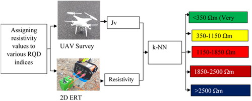
Rock quality designation (RQD) is a standard technique in mining and geotechnical investigation for quantifying the quality and degree of jointing of the rock mass. However, the need for expeditious and inexpensive geotechnical site characterization is the prime motivation for modifying RQD. This research work integrates 2D Electrical Resistivity Tomography (2D ERT) and Unmanned Aerial Vehicle (UAV) conducted at Site 1 and Site 2. The UAV survey was performed to calculate RQD on the rock surface using volumetric Joint Counts (Jv) at Sites 1 and 2. A 2D ERT survey was conducted to obtain the corresponding subsurface resistivity values. Using k-nearest neighbours (k-NN), resistivity values were assigned to various RQD indices such as very poor rocks (<350 Ωm), poor rock (350–1150 Ωm), fair rock (1150–1850 Ωm), good rock (1850–2500 Ωm) and >2500 Ωm excellent rock. Based on the established correlation of RQD and resistivity, the subsurface rock mass quality at Site 1 was predominantly good and excellent rock, while at Site 2, poor rock was significantly reported. This research concluded that rock mass characterization using RQD is more rapid and inexpensive than the direct or indirect calculation of RQD. The combined 2D ERT and UAV deployed in this research study provide an environmentally non-destructive approach for slope stability assessment.

Graphical Abstract

Keywords:

• Rock quality designation
• electrical resistivity tomography
• aerial survey
• k-nearest neighbour
• granite
• slope stability

1. Introduction

Rock quality designation (RQD) is a standard technique in mining and geotechnical investigation for quantifying the quality and degree of jointing of rock mass based on the RQD index (Khurshid et al. 2022; Safari Farrokhad et al. 2022; Tsang et al. 2022). Drill core is the primary way of estimating RQD (Cheng et al. 2016; Zheng et al. 2018); although it provides reliable information at specific points, large numbers of cores are required for accurate and detailed subsurface geological descriptions, which may be excessively costly and time-consuming. Furthermore, the estimation of RQD from drill cores is orientation-biased (Hudson and Priest 1983; Choi and Park 2004; Azimian 2016; Strelec et al. 2017; Peng et al. 2019; Kring and Chatterjee 2020). Additionally, as many rock-cut slopes are located in complex morphological areas, drilling investigation is not always possible in many cases (Alemdag et al. 2022). Priest and Hudson (1976) therefore suggested the indirect estimation of RQD from discontinuity frequency, termed as scanline survey, to circumvent the limitation of core drilling. However, the calculation of RQD from the scanline survey is directional dependent; that is, the value of RQD may vary in different directions at the same site (Wu et al. 2021; Alemdag et al. 2022; Sonmez et al. 2022). To reduce the limitation of the scanline survey, Buen and Palmstrom (1982) presented a correlation between Volumetric Joint Counts (Jv) and RQD. The Jv refers to the number of joints present in a unit volume of the rock mass.

Traditional investigation techniques for estimating Jv on rock slopes, such as tape, provide incomplete and insufficient data (Zheng et al. 2018; Mineo et al. 2022). Furthermore, the manual techniques also required direct contact with rock slopes, thus making it risky on steep slopes. Hence, advanced remote sensing techniques have made extracting data regarding discontinuity spacing from 3D point clouds easier and more rapid. Currently, unmanned aerial vehicle (UAV) survey is the most often used method for geotechnical and rock engineering applications due to its capacity to provide an accurate, denser, richer, and more exact 3D point cloud (Junaid et al. 2022c). Nevertheless, UAV is a commonly applied technique for numerous rock engineering applications but suffers certain limitations. UAV is generally considered a rapid and quick technique, but estimating Jv from the UAV 3D point cloud is time-consuming, particularly for large areas. In addition, the calculation of RQD on a 3D point cloud is impossible in a highly vegetated area (Ismail et al. 2022). Furthermore, the UAV point cloud provides surface assessment only, while subsurface rock mass quality remains unexposed.

To overcome the shortcoming mentioned above, 2D Electrical Resistivity Tomography (2D ERT) provides a promising approach by offering a low-cost, reliable, advanced data collection and interpretation and a non-destructive technique for subsurface rock mass quality characterization (Sari et al. 2020; Alpaslan 2021; Attwa et al. 2021; Junaid et al. 2021, 2022a, 2022b, 2023, Gao et al. 2024). In recent decades, 2D ERT has been widely applied for numerous geotechnical assessments, primarily balancing the investigation accuracy and cost (Liu et al. 2022). The sensitivity of the rock mass resistivity to the fracturing, weathering, and presence of water and clay content in a rock mass also makes it an appropriate technique for slope stability assessment (Asriza et al. 2017; Boyle et al. 2017; Khan et al. 2017; Singh and Sharma 2022; Sari 2023). 2D ERT is an extensively applied technique for various rock engineering applications such as rock slope stability assessment (Naudet et al. 2008; Coulibaly et al. 2017; Khan et al. 2017; Falae et al. 2019), earth dam health assessment (Camarero et al. 2019; Zumr et al. 2020), landslide monitoring and slope stability assessment (Pánek et al. 2011; Urban et al. 2015; Buša et al. 2020; Carrión-Mero et al. 2021). RQD is the globally applied technique for characterizing subsurface rock mass quality. However, all the previous research lacks the evaluation of subsurface rock mass quality based on the RQD index using a 2D ERT survey. Although, few researchers have attempted to assess the subsurface rock mass quality based on the RQD index using 2D ERT (Olona et al. 2010; Junaid et al. 2019; Ishak et al. 2020; Lin et al. 2021). The primary limitation of these studies is that they are limited to selected values of RQD and did not provide a comprehensive correlation of RQD indices and resistivity. This study attempts to assign resistivity values to various RQD indices for granite rock using integrated 2D ERT, UAV and boreholes.

This study integrates 2D ERT and UAV surveys to assign resistivity values to various RQD indices. The UAV survey was conducted to reconstruct a 3D point cloud and indirectly calculate the RQD values on a rock outcrop using Jv. The purpose of the 2D ERT survey was to extract the corresponding resistivity values for various RQD indices. The k-Nearest Neighbour (k-NN) analysis was performed to assign resistivity values to various RQD indices.

2. Site description and geological setting

Two rock slopes, namely Site 1 and Site 2, were opted to achieve the desired objectives. As both sites have granitic formations; therefore, these sites were chosen.

2.1. Site 1

Site 1 is located on one of the longest expressways in Malaysia. This expressway links many major cities of Malaysia, acting as the backbone of the peninsula’s west coast. The general geology of the study area is underlain by granitic bodies of Main Range Granite ((JMG) 2014). The rock slope is a part of the Gunung Kledang range in Kinta Valley. The study area is underlain by massive and homogeneous igneous granitic rock, which forms terrain with high reliefs exceeding 700 m (Choong 2014). The Kledang Range is in the west of Kinta Valley and is about 40 km long. Figure 1(a) shows the map of peninsular Malaysia, while Figure 1(b) indicates the study area. The red lines in Figure 1(b) illustrate the resistivity lines at the top and middle of the study area.

Figure 1. Maps of the study area: (a) map of peninsular Malaysia; (b) Site 1; (c) Site 2.

2.2. Site 2

Site 2 is situated along a newly established highway in Johor, Malaysia, as shown in Figure 1(c). This highway is considered quite busy owing to the proximity of an industrial zone and many nearby villages. Referring to the ‘Johor Geological Map’ by the Mineral and Geoscience Department of Malaysia, the general geology of the study area is underlain by granitic bodies with acidic intrusion having a high content of silica ((JMG) 2014). The granitic rock is located on the eastern belt of I-type granite. According to Ghani et al. (2013), weathering and recycling processes are thought to have melted metasedimentary crust to generate the I-type granite. The elevation concerning the mean sea level at the selected site ranges from 15 to 48 m. Site 2 is shown in Figure 1(c), while the red line in Figure 1(c) represents the resistivity line on the top of the rock slope. The slope height at the study site ranges from 10 m to 15 m.

3. Methodology

The methodologies flow chart is provided in Figure 2.

Figure 2. Methodology flow chart.

3.1. UAV survey data acquisition

A quadcopter UAV system using DJI Phantom 4 v2.0 (Figure 3a) with an onboard 20 MP camera was deployed for UAV survey acquisition at sites 1 and 2. The system is wirelessly connected to the DJI iPad controller. The maximum flight time is approximately 30 min, with a maximum speed of 20 m/s. The vertical and horizontal hover accuracy of the system with GPS positioning is 0.5 and 1.5 m, respectively (dji).

Figure 3. a) DJI Phantom 4 v2.0; (b) SOUTH G1 GNSS system.

The UAV fieldwork consisted of three main steps: 1) Flight planning, 2) Ground control points (GCP) acquisition and 3) flight operation and capturing images. The flight plan of the UAV to capture images for Site 1 and Site 2 is provided in Figure 4(a) and (b), correspondingly. The images at Site 1 were captured at the height of 180–260 m with respect to Mean Sea Level (MSL), whereas, at Site 2, images were taken at a height of approximately 5–30 m. The slope height at Site 1 was 70–80 m, while at Site 2, it was 15–20 m. Therefore, the UAV was flown at a higher altitude at Site 1 than at Site 2. The positions of the GCPs at both sites were established using the Real-Time Kinematic Global Navigation Satellite System (RTK GNSS). For this purpose, the SOUTH G1 GNNS system was utilized, as depicted in Figure 3(b). A total of 6 GCP points at Site 1 and 10 at Site 2 were acquired for georeferencing and accuracy assessment of the 3D UAV point cloud. The aerial images captured at Sites 1 and 2 were 245 and 246, respectively. An overlap of 70% between adjacent images was maintained for capturing the aerial images.

Figure 4. UAV survey flight path (a) Site 1; (b) Site 2.

3.2. UAV data processing

The 3D point cloud was reconstructed from the captured images using ShapeMetriX (SMX) UAV software, following the steps discussed below (3GSM).

1. The captured aerial images were first loaded into the SMX multi-photo to reconstruct the 3D coarse point cloud using the structure from motion (sfm) technique. After loading all the captured images, the 3D coarse point cloud is reconstructed. The time needed by the software to construct a 3D coarse point cloud depends on the number of photos captured. The 3D coarse point cloud reconstruction determines the orientation and position of the camera among all photographs relative to each other and relative to the coarsely reconstructed object.

2. Once the 3D coarse point cloud is reconstructed, the region of interest (ROI) is opted manually. The purpose of choosing ROI is to remove the unwanted points to save processing time.

3. The 3D dense point cloud is constructed in the next step. The 3D dense point cloud allows for calculating the detailed object geometry, including a detailed point cloud, surface and mesh texture.

4. Finally, the georeferencing of the 3D point cloud is carried out to assess the accuracy. In this research work, the georeferencing is carried out in a Universal Transverse Mercator (UTM) coordinate system. The obtained 3D point cloud is further processed to calculate RQD, as discussed below.

3.3. 2D ERT survey

The 2D ERT survey of both sites was accomplished by deploying ABEM LS 2 resistivity meter using the Schlumberger protocol with 10 m electrode spacing at Site 1 and 3 m spacing at Site 2. The 2D ERT survey of Site 1 consisted of two lines, namely Line 1 and 2, as mentioned in Figure 1(b). All the resistivity survey lines at Site 1 were laid longitudinally. Resistivity L1 was accomplished at the top, and L2 in the middle of the rock slope. The entire Site 1 was covered using the roll-along survey technique. The length of the resistivity line L1 was 600 m, and L2 was 1000 m. A total number of 61 electrodes at L1 and 101 for L2 (one center electrode) equally spaced at 10 m in the Schlumberger protocol was utilized in this research work. At Site 2, only one resistivity line, L3, was carried out (see Figure 1c). The length of the survey line was 120 m The details of the resistivity line length, direction and electrode spacing for both sites are summarized in Table 1.

Table 1. Detail of resistivity lines.

Site	Survey line	No of electrodes	Electrode spacing (m)	Direction	Location on rock slope
Site 1	L1	61	10	Southwest to Northwest	Top
	L2	101	10	Southwest to Northwest	Middle
Site 2	L3	41	3	North to South	Top

3.4. 2D ERT data processing

The apparent resistivity data were processed using ZondRes2DInv software (Zond) to obtain the subsurface interpretation. The generation of 2D resistivity tomography is a multi-step process. First, the raw resistivity data were loaded in the ZondRes2DInv software. The data quality was assessed in the next step, and the bad data points were removed. Then, the geomodelling of the data using forward modelling followed by inversion (least square optimization technique) was carried out. In geomodelling, the subsurface is divided into many cells, and the apparent resistivity value for each block is determined. Then, the iteration of the data iteration was carried out until the optimum root mean square (RMS) error was achieved. An RMS error of 5.15%, 10.1% and 3.49% was recorded after 13, 13 and 10 iterations for resistivity lines L1, L2 and L3.

3.5. Calculation of RQD from UAV point cloud

At sites 1 and 2, vertical sections equal to slope height were obtained at 15 m intervals, as shown in Figure 5. Consequently, at Site 1, 41 vertical sections were obtained, while seven sections were obtained at Site 2. These vertical sections were further divided into 1 m*1 flat blocks to estimate Jv, as shown in Figure 5(c). Each 1 m*1 m block provides the value of Jv that was used to calculate the RQD utilizing Equation (1)(1) $$\mathit{\text{RQD}}=115-3.3\mathit{\text{Jv}}$$(1) . Equation (1)(1) $$\mathit{\text{RQD}}=115-3.3\mathit{\text{Jv}}$$(1) in this research was used as the RQD was calculated from flat blocks, and it is more appropriate for flat blocks (Zheng et al. 2020). The RQD values from Site 1 were obtained from 182 flat blocks, while 41 flat blocks at Site 2. (1) $$\mathit{\text{RQD}}=115-3.3\mathit{\text{Jv}}$$(1)

Figure 5. Vertical sections and 1 m*1 m blocks on UAV point cloud and resistivity lines (a) Site 1 (b) Site 2 (c) 1 m*1 m block representing joints and joint set spacing.

3.6. Obtaining resistivity values for various RQD indices

Similarly, as discussed above, the 2D ERT survey line was split into vertical sections with equal slope heights. These vertical sections were further divided into 1 m*1 m flat blocks. Consequently, 182 blocks were obtained at Site 1 and 41 at Site 2. Each block represents a resistivity value for the corresponding RQD values.

3.7. k-Nearest Neighbour (k-NN)

K-NN primarily aims to categorize the data into various classes (Kamran et al. 2022). In this study, the k-NN algorithm in Python was used to assign the resistivity values to various RQD indices. In the k-NN model, 224 data points were used to represent RQD and resistivity values for various RQD indices.

The k-NN classification was performed for two types of correlation, such as RQD and resistivity, and Jv and resistivity. First, all the required libraries for the k-NN classification were called in Anaconda. Next, the 224 data points representing RQD, resistivity and Jv were loaded. The next step is to choose the optimum value of ‘k’. In this study, after various trials and errors, a ‘k’ value of 3 has been opted. At ‘k’ value of 3, the k-NN modelling in this study has higher accuracy and good performance. After finalizing the ‘k’ value the k-NN, model was run between RQD and resistivity and Jv and resistivity independently.

4. Results

4.1. UAV survey

The obtained 3D point cloud of sites 1 and 2 is depicted in Figure 6(a) and (b). The doted numbered at the toe of the slopes in Figure 6(a) and (b) represent the GCP points. The GCPs at Site 1 were six, while at Site 2 were ten. These GCPs were used for georeferencing to estimate the accuracy of the 3D point cloud, as provided in Table 2 for Site 1 and Table 3 for Site 3.

Figure 6. 3D point cloud and GCPs points at both sites (a) Site 1; (b) Site 2.

Table 2. GCP accuracy assessment of Site 1.

GCP Point	Rx (m)	Ry (m)	Rz (m)
GCP13	0.019	−0.006	−0.007
GCP14	−0.015	−0.015	0.014
GCP15	−0.029	−0.038	−0.056
GCP16	0.031	0.005	0.047
GCP17	0.008	0.032	0.004
GCP18	−0.005	−0.005	−0.003

Table 3. GCP accuracy assessment of Site 2.

GCP Point	Rx (m)	Ry (m)	Rz (m)
GCP2	0.007	0.003	−0.005
GCP3	−0.008	0.003	0.004
GCP4	−0.004	0.003	−0.007
GCP5	0.004	−0.008	0.021
GCP6	0.006	0.003	−0.012
GCP8	−0.061	0.059	0.012
GCP9	−0.009	−0.002	0.003
GCP10	0.021	−0.016	0.008
GCP11	0.022	−0.046	−0.061
GCP12	0.018	0.003	0.041

4.2. 2D ERT survey

The resistivity line L1 was positioned at the top of Site 1, enabling capturing 906 data points and segmenting the subsurface into 787 blocks. Figure 7(a) shows that resistivity values of 200 Ωm to more than 10,000 Ωm were obtained at L1, exposing two subsurface geological layers. These geological layers include a fresh rock with more than 2000 Ωm and a fractured rock with a resistivity of 300 to 2000 Ωm. The fresh rock is represented by dark reddish colour encircled by black dotted lines, while the greenish to yellow colour refers to fractured rock. L1 reported a fresh rock layer of 15–20 m thickness at the uppermost region. Towards the Southwest, major portion of the subsurface rock mass is the fresh rock. In contrast, the middle part of the rock mass at L1 is composed of fractured rock extending in the Northeast direction. The interpretation of resistivity line L1 shows that a high portion of the subsurface rock mass was moderately fractured, characterized by yellow colour having resistivity ranges of 1000 Ωm to 2000 Ωm.

Figure 7. 2D ERT images at Site 1. (a) L1; (b) L2.

The resistivity line L2 provided subsurface information using 1654 data points divided into 4000 blocks carried out in the middle of Site 1. As delineated in Figure 7(b), the high portion at resistivity line L2 was found in fresh rock with a resistivity value greater than 2000 Ωm, as shown by the dark red colour. Towards the northeast and southwest directions, a 15 to 20 m thick layer of moderately fractured rock was identified as represented by yellow colour encircled by black dotted lines having resistivity ranges 1000-2000 Ωm. A water content infilling in fractured rock reduces the resistivity values to 200–300 Ωm, which was discerned at the middle of the line near the surface. The same layer was also exposed towards the northeast, represented by green. Interestingly, the water-saturated zone was associated with fractured rock mass. This authenticates the existence of a water-saturated zone at L2, as the run-off water infiltrated through the fractured rock mass.

The 2D ERT tomography for all resistivity lines, i.e. L3 at Site 2, is shown in Figure 8. The subsurface resistivity values by L3 were obtained for 524 data points. The depth of investigation of L3 was around 25 m. The resistivity line L3 discerns three distinct geological layers at Site 2: clay, fractured and fresh rock. The resistivity value of these geological layers, consisting of clay, fractured rock and fresh rock, ranges from 100 Ωm −200 Ωm, 300 Ωm −200 Ωm, and greater than 2000 Ωm, respectively. A low resistivity layer (<150 Ωm) around 1 m thickness was observed at the topmost portion. This layer corresponds to the topsoil layer, composed of loose material due to the excavation process. Immediate to the topsoil layer, a 1 m thick geological layer characterized by yellow colour was identified by L3. The resistivity of this layer ranges between 800-1500 Ωm, thus categorized as a fractured rock. At a depth of around 2 m, a thick layer of 4-5 m was also discerned, marked by dark brown colour, having a resistivity greater than 2800 Ωm. This layer is characterized as a fresh rock. A highly fractured rock manifested by green colour at a depth of 6-7 m having resistivity 250-500 Ωm was also identified by L3. Pockets of low resistivity layers (<250 Ωm) were also noticed at a depth of around 9 to 10 m, represented by blue colour by L3. This layer was termed because the clay was observed during a field visit in the rock joints at the slope’s lower portion.

Figure 8. 2D ERT images at Site 2.

4.3. Obtained RQD and resistivity values

Cumulatively, 224 data points were obtained from Site 1 and Site 2, representing RQD and corresponding resistivity values. Of 224 data points, 183 were contributed by Site 1 and 41 by Site 2. The data points for very poor, fair, and good rock at Site 1 were 7, 78, 66 and 32, as provided in Figure 9(a). At Site 2, out of 41 data points, 18, 13 and 10 data points were obtained for poor, fair and good rock, respectively, as shown in Figure 9(b). Figure 9 reveals that the data points obtained in the present research comprise the RQD and corresponding resistivity values for almost all RQD indices. This confirms that these data points can be utilized to establish a correlation between RQD and resistivity value.

Figure 9. Frequency distribution of various quality of rocks (a) Site 1; (b) Site 2.

4.4. k-NN modelling

This study assigned the resistivity values to various RQD indices by opting for k value 3 in k-NN modelling. Figure 10 shows the predictor space chart of the k-NN model. Moreover, this study has also developed the predictor space chart using three input parameters: RQD, Jv and resistivity. The performance of the k-NN model is checked by various parameters such as precision, recall value, F1 score and support. The obtained values for these parameters are provided in Table 4. The precision value shows the accuracy and reliability of the model. Table 4 shows that the precision for poor rock (0.93) is higher than for good (0.86) and fair rock. (0.90). However, higher accuracy above 0.85 for all rock types shows that the k-NN model exploited in this research has high precision and reliability.

Figure 10. Predictor space chart of the k-NN model.

Table 4. k-NN performance.

Class	Precision	Recall	F1-score	Support
1 (Poor rock)	0.93	0.97	0.95	66
2 (Fair Rock)	0.86	0.76	0.81	33
3 (Good Rock)	0.90	0.93	0.92	30
Accuracy			0.91	129
Macro average	0.90	0.89	0.89	129
Weighted average	0.91	0.91	0.90	129

The recall value in k-NN modelling manifests the capability of the obtained model to identify the relevant data of the group. In this study, the recall value for the fair rock was the lowest, i.e. 0.76. Overall, the obtained recall value for all rock types is encouraging and thus proves the k-NN model is reliable.

F1- score is the harmonic mean of precision and recall. The F1 score is as essential in k-NN modelling as precision and recall. The good F1 score reflects the model has good precision and recall and vice versa. The F1 score from k-NN modelling for poor, fair and good rock is 0.95, 0.81 and 0.90 in this research work. The high F1 score proves that the k-NN modelling in this research study is reliable.

The graphical representation of the RQD and resistivity and the Jv and resistivity using K-NN is shown in Figure 11(a) and (b), respectively. A positive correlation between RQD and resistivity was noticed, whereas Jv and resistivity show a negative correlation. The k-NN modelling was successfully categorized into three distinct RQD classes: poor rock, fair rock and good rock, represented by red, green and yellow colour marks, respectively (Figure 11). The figure reflects that the resistivity of poor rock varies between 350 and 1150 Ωm, fair rock from 1150 to 1850 Ωm, and good rock from 1850 to 2500 Ωm. Figure 11(a,b) shows no correlation between Jv, resistivity, and RQD for poor and excellent rock. However, the RQD classification system shows that the RQD for very poor rock is less than 25%, and for excellent rock is greater than 90%. In the same scenario concluding Figure 11, less than 350 Ωm resistivity and greater than 2500 Ωm were assigned for very poor and excellent rock, respectively. The Jv, resistivity and RQD ranges obtained using k-NN modelling in this study are tabulated in Table 5.

Figure 11. k-NN modelling. (a) RQD and resistivity; (b) Jv and resistivity.

Table 5. Classification of Jv, RQD, and resistivity into various classes based on Deere work.

Jv	RQD (%)	Resistivity (Ωm)	Remarks
>27	18–25	<350	Very Poor
20–27	25–50	350–1150	Poor
12–20	50–75	1150–1850	Fair
11–7.5	75–90	1850–2500	Good
<7.5	90–100	>2500	Excellent

5. Discussions

This study developed an approach by integrating 2D ERT and UAV for estimating the RQD. Although, the 2D ERT results may have ambiguity, but the RQD and resistivity values obtained in the current study from sites 1 and 2 are compared with the previous studies as presented in Table 6. The table clearly reflects that the RQD and corresponding resistivity values obtained in current study is in good compromise with the previous research findings. This authenticate the 224 data points obtained in this study using integrated 2D ERT and UAV. Furthermore, Table 6 also shows that previously the correlation of RQD and resistivity were established for selected values of RQD, whereas this study extend the previous work by assigning the resistivity values to to all RQD indices.

Table 6. Comparison of RQD and resistivity values of previous studies and current study.

RQD (%)	Previous Studies Resistivity (Ohm.m)	Current Study Resistivity (Ohm.m)
0–5	52–500	300
16–20	66–800	0–300
51–55	800–3000	1150–1850
71–75	1800–2000	1150–1850
>90	>2500	>2500

Accurate characterization of subsurface rock mass quality is necessary to mitigate the economic losses, property damages, injuries, and fatalities due to rock slope instabilities. RQD is a widely applied empirical technique for preliminary assessment as it is the simplest among all rock mass classification systems. Nevertheless, the estimation of RQD from traditional boreholes gives reliable subsurface information but is limited to specific points only. At the same time, the indirect way of estimating using UAV remote sensing techniques suffers limitations of visualization in vegetated areas. 2D ERT was found to be successful in providing continuous and reliable subsurface investigation. Although few researchers have attempted to correlate the RQD and resistivity (Olona et al. 2010; Junaid et al. 2019; Ishak et al. 2020; Lin et al. 2021), However, a comprehensive and detailed correlation of RQD and resistivity for granitic rock does not exist to date.

This study effectively provides a more extensive correlation between RQD and resistivity values. Furthermore, all the previous studies deployed coring in integration with a 2D ERT survey to calculate RQD and corresponding resistivity values. In comparison, this study adopted an inexpensive and faster approach using integrated UAV and 2D ERT. Though, a 2D ERT survey independently may mislead and provide ambiguous results. However, the outcome of this research work is validated with the previous studies and, therefore, can be applied for various geotechnical site investigations. The correlation of RQD and corresponding resistivity values obtained in this study will enable the characterization of subsurface rock mass quality using a 2D ERT survey based on RQD indices, as provided in Figure 11. Based on the established correlation, as presented in Table 5, the subsurface rock mass was classified into various classes of RQD. The 2D ERT images were exported to Golden Surfer 13 software, and a unique and uniform colour was assigned to each RQD class, as shown in Figure 12. According to Figure 12, the very poor, poor, fair, good and excellent rocks are represented by light grey, cyan blue, orange, red and dark red colours. However, at Site 1, the good and excellent rock mass exists dominantly, as represented by Figure 12(a) and (b). On the other hand, Site 2 is dominantly composed of poor rock, as illustrated by Figure 12(c).

Figure 12. Subsurface rock mass quality characterization. (a) L1; (b) L2; (c) L3.

Figure 12 shows a thorough insight into rock mass quality at both sites compared to the ERT interpretations presented in Figures 7 and 8. The 2D ERT interpretation classifies the subsurface rock mass as a fresh and fractured rock. Whereas the correlation between RQD and resistivity established in this study categorized the rock mass into five classes based on RQD indices. This shows that the outcome of current research studies provides a more extensive subsurface rock mass quality investigation along the rock slope. As mentioned in Figure 12, the lateral and vertical extent of various subsurface rock mass quality is efficiently identified. This information can be relied on to take the necessary actions to mitigate rock falls due to slope instabilities.

Furthermore, the approach developed in this study for subsurface rock mass quality characterization optimize the cost of investigation. A detailed subsurface geological investigation were carried out using inexpensive and expeditious 2D ERT survey compared to core drilling. Thus, this research offers an expeditious, effective, inexpensive and environmentally non-destructive approach for subsurface rock mass characterization based on RQD using 2D ERT. Granitic rocks may have different resistivity in various regions. However, the resistivity values assigned to various RQD indices are in a wider range in this research work. Therefore, it is believed that the resistivity of granitic rock from anywhere will exist in these specific ranges. Therefore, the correlation of RQD and resistivity obtained in this study has applicability to all granitic rock types. Hence, the approach of this study is applicable in most cases.

6. Conclusion

This study successfully compares and correlates resistivity values with various RQD indices, which was achieved by utilizing k-NN, modelling on 224 data points obtained using 2D ERT and UAV surveys. The conclusion based on this research study is summarized as follows:

1. The study effectively assigned the resistivity values to various RQD indices such as very poor rocks (<350 Ωm), poor rock (350–1100 Ωm), fair rock (1100–1950 Ωm), good rock (1950–2400 Ωm) and >2400 Ωm excellent rock.

2. The obtained correlation of RQD and resistivity values in the current study was successfully validated with previous studies, thus authenticates the outcome of this study.

3. The resistivity of the rock mass decreases with an increase in the degree of fracturing.

4. A reciprocal relationship was identified between the resistivity and Jv, indicating that a higher Jv causes a decrease in resistivity and vice versa.

5. A direct proportionality was found between the resistivity and RQD, showing that an increase in the RQD is associated with an increase in the resistivity of the rock mass.

6. Based on the established correlation of RQD and resistivity, the subsurface rock mass quality at Site 1 was predominantly good and excellent rock, while at Site 2, poor rock was significantly reported.

7. The calculation of RQD, either by direct or indirect technique, provides spotted information or may overlook the rock mass quality, while a geophysical survey provides continuous subsurface information.

8. The subsurface characterization of rock mass quality using 2D ERT is expeditious, inexpensive and environmentally non-destructive.

9. The study provides a paradigm for detail subsurface rock mass quality evaluation using 2D ERT.

The correlation of RQD with other geophysical techniques can be established to increase the reliability of the data and subsurface investigation. Furthermore, the correlation of RQD and resistivity with other rock mass classifications may be attempted.

Acknowledgment

The authors express their deep appreciation and gratitude towards the Researchers Supporting Project, King Saud University, Riyadh, Saudi Arabia, under Project Number RSP2024R351, for their financial support of this research article. Additionally, heartfelt thanks are extended to the Higher Education Commission of Pakistan and Universiti Teknologi Malaysia for their contributions towards facilitating this study. Special acknowledgment is also given to 3GSM for generously providing a complimentary educational license for the SMX UAV software. All the authors are extremely thankful to Dr. Sajid Mahmood for his efforts in improving the discussion section of article and removing linguistic mistakes.

Data availability statement

The datasets generated during and/or analyzed during the current study are available from the corresponding author upon reasonable request.

Disclosure statement

The authors declare no relevant financial or nonfinancial interests to disclose.

References

- 3GSM. https://3gsm.at/.
- (JMG), M. a. G. d. 2014. Geological map of peninsular Malaysia. (Peta Geologi Semenanjung). https://www.jmg.gov.my/add_on/mt/smnjg/tiles/.
- Alemdag S, Sari M, Seren A. 2022. Determination of rock quality designation (RQD) in metamorphic rocks: a case study (Bayburt-Kırklartepe Dam). Bull Eng Geol Environ. 81(5):214. doi: 10.1007/s10064-022-02675-2.
- Alpaslan N. 2021. Determination of borehole locations and saline-water intrusion for groundwater in Central Anatolia Region, Turkey using electrical tomography (ERT) method. Environ Earth Sci. 80(24):810. doi: 10.1007/s12665-021-10117-7.
- Asriza S, Kristyanto T, Indra T, Syahputra R, Tempessy A. 2017. Determination of the landslide slip surface using electrical resistivity tomography (ERT) technique. Paper presented at the Advancing Culture of Living with Landslides: Vol. 2, Advances in Landslide Science: 53.
- Attwa M, El Bastawesy M, Ragab D, Othman A, Assaggaf HM, Abotalib AZ. 2021. Toward an integrated and sustainable water resources management in structurally-controlled watersheds in desert environments using geophysical and remote sensing methods. Sustainability. 13(7):4004. doi: 10.3390/su13074004.
- Azimian A. 2016. A new method for improving the RQD determination of rock core in borehole. Rock Mech Rock Eng. 49(4):1559–1566. doi: 10.1007/s00603-015-0789-8.
- Boyle A, Wilkinson PB, Chambers JE, Meldrum PI, Uhlemann S, Adler A. 2017. Jointly reconstructing ground motion and resistivity for ERT-based slope stability monitoring. Geophys J Int. 212(2):1167–1182. doi: 10.1093/gji/ggx453.
- Buen B, Palmstrom A. 1982. Design and supervision of unlined hydro power shafts and tunnels with head up to 590 meters. Paper presented at the ISRM international symposium. Aachen, Germany, May 1982.
- Buša J, Rusnák M, Kušnirák D, Greif V, Bednarik M, Putiška R, Dostál I, Sládek J, Rusnáková D. 2020. Urban landslide monitoring by combined use of multiple methodologies-a case study on Sv. Anton town, Slovakia. Phys Geogr. 41(2):169–194. doi: 10.1080/02723646.2019.1630232.
- Camarero PL, Moreira CA, Pereira HG. 2019. Analysis of the physical integrity of earth dams from electrical resistivity tomography (ERT) in Brazil. Pure Appl Geophys. 176(12):5363–5375. doi: 10.1007/s00024-019-02271-8.
- Carrión-Mero P, Briones-Bitar J, Morante-Carballo F, Stay-Coello D, Blanco-Torrens R, Berrezueta E. 2021. Evaluation of slope stability in an urban area as a basis for territorial planning: a case study. Appl Sci. 11(11):5013. doi: 10.3390/app11115013.
- Cheng C, Li X, Li S, Zheng B. 2016. Geomechanical studies on granite intrusions in Alxa area for high-level radioactive waste disposal. Sustainability. 8(12):1329. doi: 10.3390/su8121329.
- Choi S, Park H. 2004. Variation of rock quality designation (RQD) with scanline orientation and length: a case study in Korea. Int J Rock Mech Min Sci. 41(2):207–221. doi: 10.1016/S1365-1609(03)00091-1.
- Choong CM. Structural History of the Kinta Valley, MSc Thesis, Geoscience Dept., Faculty of Geoscience and Petroleum; 2014.
- Coulibaly Y, Belem T, Cheng L. 2017. Numerical analysis and geophysical monitoring for stability assessment of the Northwest tailings dam at Westwood Mine. Int J Min Sci Technol. 27(4):701–710. doi: 10.1016/j.ijmst.2017.05.012.
- dji. https://www.dji.com/phantom-4-pro-v2.
- Falae PO, Kanungo D, Chauhan P, Dash RK. 2019. Recent trends in application of electrical resistivity tomography for landslide study. Paper presented at the Renewable Energy and Its Innovative Technologies. Proceedings of ICEMIT 2017, Volume 1. Springer; p. 195–204.
- Gao Q, Hasan M, Shang Y, Qi S. 2024. Geophysical estimation of 2D hydraulic conductivity for groundwater assessment in hard rock. Acta Geophys. 1–12. doi: 10.1007/s11600-024-01310-w.
- Ghani AA, Searle M, Robb L, Chung S-L. 2013. Transitional IS type characteristic in the main range granite, Peninsular Malaysia. J Asian Earth Sci. 76:225–240. doi: 10.1016/j.jseaes.2013.05.013.
- Hudson J, Priest S. 1983. Discontinuity frequency in rock masses. Int J Rock Mech Min Sci Geomech Abstr, Elsevier. 20(2):73–89. doi: 10.1016/0148-9062(83)90329-7.
- Ishak MF, Zaini MI, Zolkepli M, Wahap M, Sidek JJ, Yasin AM, Zolkepli M, Sidik MM, Arof KM, Talib ZA. 2020. Granite exploration by using electrical resistivity imaging (ERI): a case study in Johor. Int J Integr Eng. 12(8):328–347.
- Ismail A, A Rashid AS, Sa’ari R, Rasib AW, Mustaffar M, Abdullah RA, Kassim A, Mohd Yusof N, Abd Rahaman N, Mohd Apandi N, et al. 2022. Application of UAV-based photogrammetry and normalised water index (NDWI) to estimate the rock mass rating (RMR): a case study. Phys Chem Earth Parts A/B/C. 127:103161. doi: 10.1016/j.pce.2022.103161.
- Junaid M, Abdullah RA, Sa’ari R, Ali W, Islam A, Sari M. 2022a. 3D modelling and feasibility assessment of granite deposit using 2D electrical resistivity tomography, borehole, and unmanned aerial vehicle survey. J Min Environ. 13(4):929–942.
- Junaid M, Abdullah RA, Sa’ari R, Ali W, Rehman H, Alel MNA, Ghani U. 2021. 2D Electrical Resistivity Tomography an advance and expeditious exploration technique for current challenges to mineral industry. J Himal Earth Sci. 54(1):11–32.
- Junaid M, Abdullah RA, Sa’ari R, Ali W, Rehman H, Shah k S, Sari M. 2022b. Water-saturated zone recognition using integrated 2D electrical resistivity tomography, borehole, and aerial photogrammetry in granite deposit, Malaysia. Arab J Geosci. 15(14):1301. doi: 10.1007/s12517-022-10572-x.
- Junaid M, Abdullah RA, Sa’ari R, Rehman H, Shah KS, Ullah R, Alel MNA, Zainal IZ, Zainuddin NE. 2022c. Quantification of rock mass condition based on fracture frequency using unmanned aerial vehicle survey for slope stability assessment. J Indian Soc Remote Sens. 50(11):2041–2054.
- Junaid M, Abdullah RA, Sa’ari R, Shah KS, Ullah R. 2023. A comparative study of the influence of volumetric joint counts (Jv) and resistivity on rock quality designation (RQD) using multiple linear regression. Pure Appl Geophys. 180(6):2351–2368. doi: 10.1007/s00024-023-03260-8.
- Junaid M, Abdullah RA, Saa’ri R, Alel M, Ali W, Ullah A. 2019. Recognition of boulder in granite deposit using integrated borehole and 2D electrical resistivity imaging for effective mine planning and development.
- Kamran M, Ullah B, Ahmad M, Sabri MMS. 2022. Application of KNN-based Isometric Mapping and Fuzzy C-Means Algorithm to Predict Short-term Rockburst Risk in Deep Underground Projects.
- Khan MS, Hossain S, Ahmed A, Faysal M. 2017. Investigation of a shallow slope failure on expansive clay in Texas. Eng Geol. 219:118–129. doi: 10.1016/j.enggeo.2016.10.004.
- Khurshid MN, Khan AH, Rehman Z u, Chaudhary TS. 2022. The evaluation of rock mass characteristics against seepage for sustainable infrastructure development. Sustainability. 14(16):10109. doi: 10.3390/su141610109.
- Kring K, Chatterjee S. 2020. Uncertainty quantification of structural and geotechnical parameter by geostatistical simulations applied to a stability analysis case study with limited exploration data. Int J Rock Mech Min Sci. 125:104157. doi: 10.1016/j.ijrmms.2019.104157.
- Lin D, Yuan R, Lin X, Lin X, Lou C, Cai Y, Yu J, Qiu R, Su X, Wang H. 2021. Disturbed granite identification by integrating rock mass geophysical properties. Int J Rock Mech Min Sci. 138:104596. doi: 10.1016/j.ijrmms.2020.104596.
- Liu X, Shen J, Yang M, Cai G, Liu S. 2022. Subsurface characterization of a construction site in Nanjing, China using ERT and CPTU methods. Eng Geol. 299:106563. doi: 10.1016/j.enggeo.2022.106563.
- Mineo S, Caliò D, Pappalardo G. 2022. UAV-based photogrammetry and infrared thermography applied to rock mass survey for geomechanical purposes. Remote Sens. 14(3):473. doi: 10.3390/rs14030473.
- Naudet V, Lazzari M, Perrone A, Loperte A, Piscitelli S, Lapenna V. 2008. Integrated geophysical and geomorphological approach to investigate the snowmelt-triggered landslide of Bosco Piccolo village (Basilicata, southern Italy). Eng Geol. 98(3-4):156–167. doi: 10.1016/j.enggeo.2008.02.008.
- Olona J, Pulgar JA, Fernández‐Viejo G, López‐Fernández C, González‐Cortina JM. 2010. Weathering variations in a granitic massif and related geotechnical properties through seismic and electrical resistivity methods. Near Surf Geophys. 8(6):585–599. doi: 10.3997/1873-0604.2010043.
- Pánek T, Tábořík P, Klimeš J, Komárková V, Hradecký J, Šťastný M. 2011. Deep-seated gravitational slope deformations in the highest parts of the Czech Flysch Carpathians: evolutionary model based on kinematic analysis, electrical imaging and trenching. Geomorphology. 129(1-2):92–112. doi: 10.1016/j.geomorph.2011.01.016.
- Peng D, Xu Q, Zhang X, Xing H, Zhang S, Kang K, Qi X, Ju Y, Zhao K. 2019. Hydrological response of loess slopes with reference to widespread landslide events in the Heifangtai terrace, NW China. J Asian Earth Sci. 171:259–276. doi: 10.1016/j.jseaes.2018.12.003.
- Priest SD, Hudson J. 1976. Discontinuity spacings in rock. Paper presented at the International Journal of Rock Mechanics and Mining Sciences & Geomechanics Abstracts.
- Safari Farrokhad S, Lashkaripour GR, Hafezi Moghaddas N, Aligholi S, Sabri MMS. 2022. The effect of the petrography, mineralogy, and physical properties of limestone on Mode I fracture toughness under dry and saturated conditions. Appl Sci. 12(18):9237. doi: 10.3390/app12189237.
- Sari M. 2023. Evaluation of stability in rock-fill dams by numerical analysis methods: a case study (Gümüşhane-Midi Dam, Türkiye). Baltica. 36(7–12):89–99. doi: 10.5200/baltica.2023.2.1.
- Sari M, Seren A, Alemdag S. 2020. Determination of geological structures by geophysical and geotechnical techniques in Kırklartepe Dam Site (Turkey). J Appl Geophys. 182:104174. doi: 10.1016/j.jappgeo.2020.104174.
- Singh U, Sharma PK. 2022. Seasonal groundwater monitoring using surface NMR and 2D/3D ERT. Environ Earth Sci. 81(7):1–17. doi: 10.1007/s12665-022-10325-9.
- Sonmez H, Ercanoglu M, Dagdelenler G. 2022. A novel approach to structural anisotropy classification for jointed rock masses using theoretical rock quality designation formulation adjusted to joint spacing. J Rock Mech Geotech Eng. 14(2):329–345. doi: 10.1016/j.jrmge.2021.08.009.
- Strelec S, Mesec J, Grabar K, Jug J. 2017. Implementation of in-situ and geophysical investigation methods (ERT & MASW) with the purpose to determine 2D profile of landslide. Acta Montan Slovaca. 22(4):345.
- Tsang L, He B, Rashid ASA, Jalil AT, Sabri MMS. 2022. Predicting the Young’s modulus of rock material based on petrographic and rock index tests using boosting and bagging intelligence techniques. Appl Sci. 12(20):10258. doi: 10.3390/app122010258.
- Urban J, Pánek T, Hradecký J, Tábořík P. 2015. Deep structures of slopes connected with sandstone crags in the upland area of the Świętokrzyskie (Holy Cross) Mountains, Central Poland. Geomorphology. 246:519–530. doi: 10.1016/j.geomorph.2015.06.048.
- Wu F, Wu J, Bao H, Li B, Shan Z, Kong D. 2021. Advances in statistical mechanics of rock masses and its engineering applications. J Rock Mech Geotech Eng. 13(1):22–45. doi: 10.1016/j.jrmge.2020.11.003.
- Zheng J, Wang X, Lü Q, Liu J, Guo J, Liu T, Deng J. 2020. A contribution to relationship between volumetric joint count (J v) and rock quality designation (RQD) in three-dimensional (3-D) space. Rock Mech Rock Eng. 53(3):1485–1494. doi: 10.1007/s00603-019-01986-3.
- Zheng J, Yang X, Lü Q, Zhao Y, Deng J, Ding Z. 2018. A new perspective for the directivity of Rock Quality Designation (RQD) and an anisotropy index of jointing degree for rock masses. Eng Geol. 240:81–94. doi: 10.1016/j.enggeo.2018.04.013.
- Zumr D, David V, Jeřábek J, Noreika N, Krása J. 2020. Monitoring of the soil moisture regime of an earth-filled dam by means of electrical resistance tomography, close range photogrammetry, and thermal imaging. Environ Earth Sci. 79(12):1–11. doi: 10.1007/s12665-020-09052-w.