Kronecker Sequences with Many Distances

Abstract

The three gap theorem states that for any $\alpha \in \mathbb{R}$ and $N\in \mathbb{N}$, the number of different gaps between consecutive $\mathit{n\alpha }(\mathrm{\text{mod }}1)$ for $n\in \{1,\dots ,N\}$ is at most 3. Biringer and Schmidt (2008) instead considered the distance from each point to its nearest neighbor, generalizing to higher dimensions. We denote the maximum number of distances in ${\mathbb{T}}^d$ using the p-norm by ${\overline{g}}_p^d$ so that ${\overline{g}}_p^1=3$. Haynes and Marklof (2021) showed that each example with arbitrary α and N gives a generic lower bound, and that ${\overline{g}}_2^2=5$ and ${\overline{g}}_2^d\le {\sigma }_d+1$ where σ_d is the kissing number. They gave an example showing ${\overline{g}}_2^3\ge 7$. Our examples that show ${\overline{g}}_2^3\ge 9$ and also ${\overline{g}}_2^4\ge 11,{\overline{g}}_2^5\ge 13$ and ${\overline{g}}_2^6\ge 14$. Haynes and Ramirez (2021) showed that ${\overline{g}}_{\infty }^d\le 2^d+1$ and that this is sharp for $d\le 3$. We provide a numerical example to show ${\overline{g}}_{\infty }^4\ge 15$, and a proof that ${\overline{g}}_{\infty }^d\ge 2^{d-1}+1$ in general. Results for $p=\infty$ and σ_d imply that ${\overline{g}}_p^d$ depends on p for $d\ge 11$ and we conjecture this for $d\ge 4$. For $d\le 3$ we expect that ${\overline{g}}_p^d=\{3,5,9\}$ for $d=\{1,2,3\}$ respectively, independent of p. For d = 1 this is trivial, for d = 2 we show that ${\overline{g}}_p^2\ge 5$ and for d = 3 we provide numerical examples suggesting that ${\overline{g}}_p^3\ge 9$.

KEYWORDS:

• Kronecker sequences
• p-norm
• three gap theorem
• kissing number

1 Introduction

What is the maximum local complexity for equally spaced points on a torus ${\mathbb{T}}^d$ (defined in Section 2)? Equally spaced refers to the set ${\left\{n\alpha \right\}}_{1\le n\le N}$ for fixed $\alpha \in {\mathbb{T}}^d$. Local complexity refers to the number of different neighborhoods of each of the points, suitably defined; see for example [5]. The three gap theorem states that if d = 1 and the local complexity refers to the smallest distance to a point on the right, that is, gap distances between consecutive points, the maximum local complexity is three. It was proved by Sós [8, 9] and independently by Swierczkowski [10] and has many alternative proofs and generalizations.

Biringer and Schmidt [1] noted that a slightly weaker version, the three distance theorem, applies if the gap (distance to the right) is replaced by the nearest neighbor distance, and that this has a natural generalization to higher dimensions. They then considered Riemannian manifolds, where the equally spaced points could generalize to isometries of the manifold, or equally spaced points on a geodesic. In our case (the torus) they give an upper bound ${\overline{g}}_2^d\le 3^d+1$, where distance is induced from the usual Euclidean metric. We use the notation ${\overline{g}}_p^d$ (with ($p\in [1,\infty ]$) for the maximum number of distinct distances for the p-norm on ${\mathbb{T}}^d$ and $g_p^d(\alpha ,N)$ for the number of distinct distances for a particular α and N. See Section 2 for the precise definitions. Note that Biringer and Schmidt start their sequences from zero rather than one, so their N values (denoted n in their paper) are one smaller.

Haynes and Marklof [3] proved that ${\overline{g}}_2^2=5,{\overline{g}}_2^3\ge 7$ and ${\overline{g}}_2^d\le {\sigma }_d+1$ where σ_d is the kissing number, the maximum number of equal radius balls that can touch a single ball in d dimensions. In the dimensions considered in our examples, it is known that ${\sigma }_3=12,{\sigma }_4=24,40\le {\sigma }_5\le 44$ and $72\le {\sigma }_6\le 78$ [2, 6]. See also Lemma 3.

Haynes and Marklof also showed in their Theorem 2 that (1) $$\underset{i\to \infty }{\mathrm{\text{lim}}\sup }{g}_2^d(\alpha \prime ,N_i,\Lambda \prime )\ge \underset{N}{\mathrm{\text{sup}}}{g}_2^d(\alpha ,N,\Lambda )$$(1) for all α, all non-degenerate lattices Λ and $\Lambda \prime$, all subexponential sequences $\left\{N_i\right\}$ and almost all $\alpha \prime$. Thus an example for ${\mathbb{T}}^d$ (based on the cubic lattice ${\mathbb{Z}}^d$) with arbitrary α and N gives a generic lower bound for tori based on all lattices.

This theorem in Ref. [3] uses the Euclidean norm. However, its proof relies on showing that there is an open set of lattices which obtain the upper bound on the number of distances. This is a topological property of the space and the functions involved and it is not hard to see from this point of view that the same proof will work, with only minor modifications, for any norm which induces the same topology, including the maximum norm and other p-norms (Alan Haynes and Jens Marklof, private communication).

Our numerical methods for finding these examples and hence lower bounds on ${\overline{g}}_p^d$ are as follows:

Random search We sample about 10¹² values of α uniformly in ${\mathbb{T}}^d$ and find most of the examples presented here.

Rational search We can exhaustively search α with denominator up to some limit, around 2000 for d = 3 and 200 for d = 6.

Lattice search Searching near a known solution extended the number of distances for p = 2, d = 6 from 13 to 14. In addition, evaluating the number of distances on a lattice in α in the vicinity of a solution is used to estimate the d-volume of the domain of that solution.

Mathematica was used to verify solutions; see the Appendix. It was also used to find the area of the pentagonal region of the example for $p=\infty$, d = 2. In addition, rigorous constructions of solutions were used in the proofs of Theorems 2 and 5. Both the rational search and the Mathematica verification may be considered rigorous claims, conditional on the software being free of bugs that materially affect the results. The author’s own code was written in C++, in some cases extended to GPU code by Mark Pearson (see the Acknowledgments).

For the Euclidean norm, we provide new examples for $3\le d\le 6$ that were obtained numerically, hence improving the lower bounds for ${\overline{g}}_2^d$. We also note that any example in a given dimension d is also an example for any larger dimension, that is, ${\overline{g}}_2^d$ is a non-decreasing function of d. In summary:

Theorem 1.

(2) $${\overline{g}}_2^d\ge \{\begin{array}{cc}9& d=3\\ 11& d=4\\ 13& d=5\\ 14& d\ge 6\end{array}$$(2)

Remark

s:

1. The examples for $4\le d\le 6$ were found using Mark Pearson’s code (see the Acknowledgments).

2. Whilst a significant improvement on the previous bound ${\overline{g}}_2^d\ge 7$ for these dimensions, there is still some distance between these and the upper bound ${\sigma }_d+1$.

3. Since all lattices can be used for finding examples, it is possible to consider lattices of higher symmetry. We have tried the F₄ lattice for d = 4, that is, the lattice with an extra point at the center of every 4-cube. However this does not seem to be more efficient in finding examples.

4. The case of few distances has also been studied: Weiß [11] found $\alpha \in {\mathbb{T}}^d$ for d = 2, 3 for which $g_2^d(\alpha ,N)=1$ for infinitely many N.

Haynes and Ramirez [4] consider instead the maximum metric, that is, based on the $\infty$-norm. These authors give an upper bound ${\overline{g}}_{\infty }^d\le 2^d+1$ for the equivalent maximum number of distances and show it is sharp for d = 2, 3 (as well as d = 1). They did not find any examples to show ${\overline{g}}_{\infty }^4>9$. We can improve this as follows, using a numerical example for d = 4 and a general construction for $d\ge 5$:

Theorem 2.

(3) $${\overline{g}}_{\infty }^d\ge \{\begin{array}{cc}15& d=4\\ 2^{d-1}+1& d\ge 5\end{array}$$(3)

Now we obtain a closed form bound on the kissing number

Lemma 3.

(4) $${\sigma }_d<\frac{d(d-1)2^{d/2}}{(\sqrt{2}-1)\sqrt{\pi }},\mathrm{\hspace{1em}}\mathrm{\hspace{1em}}d\ge 3$$(4)

This is not a particularly tight bound or difficult to prove, but we include it here as the bounds we found in the literature involved integrals or special functions, so it may be of independent interest.

Combining Theorem 2 and Lemma 3 we show

Theorem 4.

(5) $${\overline{g}}_{\infty }^d>{\overline{g}}_2^d,\mathrm{\hspace{1em}}\mathrm{\hspace{1em}}d\ge 11$$(5)

Remark

s:

1. For the dimensions in which Theorem 4 holds, this shows that ${\overline{g}}_p^d$ depends on p.

2. We conjecture that Theorem 4 holds for $d\ge 4$. For d < 4, see below.

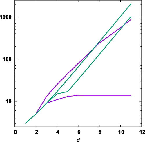
The new lower bounds on ${\overline{g}}_2^d$ and ${\overline{g}}_{\infty }^d$ together with previously known upper bounds are illustrated in Figure 1.

Fig. 1 The best current upper and lower bounds for the maximum number of distances in the Euclidean norm (${\overline{g}}_2^d$, purple) and the maximum norm (${\overline{g}}_{\infty }^d$, green) as a function of the dimension.

Finally, we consider general p-norms in low dimension and can show

Theorem 5.

For all p-norms with $p\in [1,\infty ],g_p^2\ge 5$.

Remark:

We also have examples (presented in Section 8) giving numerical evidence that $g_p^3\ge 9$ for all p. We conjecture that $g_p^2=5$ and $g_p^3=9$, independent of p, in contrast to higher dimensions.

In Section 2 we define the torus and its norms and metrics. We also recall the calculation of the number of distances from Ref. [3]. In Section 3 we give examples for the Euclidean norm for $1\le d\le 6$, including those needed to prove Theorem 1, as well as some others of minimal length and/or denominator. In Section 4 we give examples for the maximum metric. In Section 5 we prove Theorem 1, then, in Section 6 we provide the example and proof for Theorem 2. Section 7 provides the proofs of Lemma 3 and Theorem 4. Finally, for general p-norms, Theorem 5 for d = 2 is proved, and the examples for d = 3 are presented in Section 8.

2 Preliminaries

The torus ${\mathbb{T}}^d={\mathbb{R}}^d/{\mathbb{Z}}^d$ is the d-dimensional Euclidean space, identifying each point $x\in {\mathbb{R}}^d$ with its lattice translates $x+{\mathbb{Z}}^d$. It is easy to see for $x,y\in {\mathbb{T}}^d$ and $n\in \mathbb{Z}$ that nx, x + y and x–y are well defined under this identification.

The p-norm on ${\mathbb{R}}^d$ for $p\in [1,\infty ]$, denoted $|·{|}_p$, is defined as (6) $$|x{|}_p=\{\begin{array}{cc}{\left(\sum _{j=1}^d|x_j{|}^p\right)}^{1/p}& p<\infty \\ {\mathrm{\text{max}}}_{1\le j\le d}\left|x_j\right|& p=\infty \end{array}$$(6)

For p = 2 this is the Euclidean norm, whilst for $p=\infty$ it is the maximum norm.

This induces the following norm on ${\mathbb{T}}^d$: (7) $$\mathit{⏧x}{⏧}_p=\underset{z\in {\mathbb{Z}}^d}{\mathrm{\text{min}}}|x-z{|}_p$$(7)

that in turn induces the metric (8) $${\mathrm{d}}_p(x,y)=\underset{z\in {\mathbb{Z}}^d}{\mathrm{\text{min}}}|x-y-z{|}_p=\mathit{⏧x}-y{⏧}_p$$(8) giving our notion of distance on the torus. When d = 1 and when considering a single component in higher dimensions, all the norms and distances are equivalent, so the p will be omitted from the notation. When d = 2, the “disk” of fixed radius for p = 1 and for $p=\infty$ is a square, and these correspond to the same metric in different lattices, thus ${\overline{g}}_1^2={\overline{g}}_{\infty }^2$.

We also define $N_{n,j}$ to be the distance to the nearest integer (that is, the norm on ${\mathbb{T}}^1$) of $n{\alpha }_j$, where α_j is the jth component of α, so that (9) $$\mathit{⏧n\alpha }{⏧}_p=\{\begin{array}{cc}{\left(\sum _{j=1}^d{N}_{n,j}^p\right)}^{1/p}& p<\infty \\ {\mathrm{\text{max}}}_{1\le j\le d}{N}_{n,j}& p=\infty \end{array}$$(9)

We are interested in the distance (according to ${\mathrm{d}}_p$) from the point $\mathit{i\alpha }$ to its nearest neighbor where $1\le i\le N$, that is (10) $${\mathrm{d}}_p^{\mathit{\text{nn}}}(\alpha ,N,i)=\underset{\begin{array}{c}1\le j\le N\\ j\ne i\end{array}}{\mathrm{\text{min}}}{\mathrm{d}}_p(\mathit{i\alpha },\mathit{j\alpha })$$(10)

the number of distinct nearest neighbor distances (11) $$g_p^d(\alpha ,N)=\#\left\{{\mathrm{d}}_p^{\mathit{\text{nn}}}(\alpha ,N,i):1\le i\le N\right\}$$(11)

and its maximum value (12) $${\overline{g}}_p^d=\underset{\alpha ,N}{\mathrm{\text{max}}}{g}_p^d(\alpha ,N)$$(12)

Given that ${\mathrm{d}}_p(\mathit{i\alpha },\mathit{j\alpha })={\mathrm{d}}_p(0,|j-i|\alpha )=⏧|j-i|\alpha {⏧}_p$ it is easy to see (and noted in Ref. [3]) that this is (13) $${\mathrm{d}}_p^{\mathit{\text{nn}}}(\alpha ,N,i)=\underset{1\le k\le n}{\mathrm{\text{min}}}\mathit{⏧k\alpha }{⏧}_p\equiv {\delta }_p(\alpha ,n),\mathrm{\hspace{1em}}\mathrm{\hspace{1em}}n=\{\begin{array}{cc}N-i& 1\le i\le \frac{N+1}{2}\\ i-1& \frac{N+1}{2}\le i\le N\end{array}$$(13) where $k=|j-i|$. Now, as i ranges from 1 to N, ${\delta }_p(\alpha ,n)$ has its largest value for $n=\lfloor \frac{N}{2}\rfloor$ and decreases as n is increased to N–1. The number of distinct nearest neighbor distances is thus: (14) $$g_p^d(\alpha ,N)=\#\left\{n:\lfloor \frac{N}{2}\rfloor +1\le n\le N-1,{\delta }_p(\alpha ,n)<{\delta }_p(\alpha ,n-1)\right\}+1$$(14)

All but one of the minimum distances occur for $n>\frac{N-1}{2}$, which implies that (15) $$N\ge 2g_p^d-1.$$(15)

for all α. For examples where this bound is sharp, see Sections 3.7 and 4.5.

Where possible, we seek the simplest examples, which are hopefully also the most illustrative. So, for each d, we seek the largest $g_p^d(\alpha ,N)$, then the smallest N, then the α with the smallest denominator. Symmetry allows us to permute the coordinates and to replace α_i by $1-{\alpha }_i$ so each solution belongs to an equivalence class of $d!2^d$ solutions (or fewer if it has symmetry). Henceforth we assume without loss of generality that $0\le {\alpha }_1\le \cdots \le {\alpha }_d\le 1/2$.

3 Examples for the Euclidean norm

3.1 d = 1

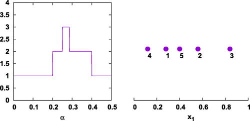
We have ${\overline{g}}^1=3$ as previously reported and can achieve N = 5, the minimum possible value from equation (15)(15) $$N\ge 2g_p^d-1.$$(15) . The only possible decreasing sequence of distances is $\mathrm{\text{min}}(\mathit{⏧\alpha ⏧},⏧2\mathit{\alpha ⏧})>⏧3\mathit{\alpha ⏧}>⏧4\mathit{\alpha ⏧}$ which yields easily the solution set $1/4<\alpha <2/7$ of size $1/28\approx 0.0357$ (ignoring the $\alpha >1/2$ region as noted above). The simplest rational example is $\alpha =\frac{3}{11}$ (found by exhaustive rational search, numerically or manually) for which $\mathit{\text{⏧nα⏧}}=\frac{1}{11}\{\mathbf{3},5,\mathbf{2},\mathbf{1}\}$ for $n=\{1,2,3,4\}$, respectively, with the relevant distances in bold. A plot of $g_1(\alpha ,5)$ and example with three distances is shown in Figure 2. There are no examples with smaller denominator but higher length N.

Fig. 2 Left: plot of $g^1(\alpha ,5)$. Right: the Kronecker sequence for $\alpha =0.28$, showing three shortest distances, $d(\alpha ,5\alpha )<d(2\alpha ,5\alpha )<d(2\alpha ,3\alpha )$.

3.2 d = 2

As noted in Ref. [3], we have ${\overline{g}}_2^2=5$, and can achieve N = 9 with $\alpha =(0.132,0.38)$ (see their fig. 2). Again, this is the minimum possible N according to equation (15)(15) $$N\ge 2g_p^d-1.$$(15) . Numerically, this example is in the only region where this N exists (modulo symmetry), a roughly triangular region with area about $1.5109\times {10}^{-6}$; see Figure 3. The solution with minimal denominator for this length is: $$\alpha =\left(\frac{15}{113},\frac{43}{113}\right)$$which has a decimal approximation $(0.1327\dots ,0.3805\dots )$. For this example we find $\mathit{⏧n\alpha }{⏧}^2={113}^{-2}\{2074,\mathbf{1629},2281,5725$, $\mathbf{1563},\mathbf{1553},\mathbf{1508},\mathbf{74}\}$ for $1\le n\le 8$, with the relevant distances in bold. The boundary of the region occurs when any of the inequalities $⏧2\mathit{\alpha ⏧}>⏧5\mathit{\alpha ⏧}>⏧6\mathit{\alpha ⏧}>|7\mathit{\alpha ⏧}>⏧8\mathit{\alpha ⏧}$ is broken. Here, $⏧8\mathit{\alpha ⏧}$ is much smaller than $⏧7\mathit{\alpha ⏧}$, so that the boundaries of the region are the circular arcs defined by $⏧2\mathit{\alpha ⏧}=⏧5\mathit{\alpha ⏧},⏧5\mathit{\alpha ⏧}=⏧6\mathit{\alpha ⏧}$ and $⏧6\mathit{\alpha ⏧}=⏧7\mathit{\alpha ⏧}$. See Figure 4.

Fig. 3 Upper left: plot of $g_2^2(\alpha ,9)$ in the α plane. The color (black for 1 to yellow for 5) indicates $g_2^2(\alpha ,9)$, that is, the number of distinct shortest distances for N = 9, the given α and Euclidean metric. The region with five distances is too small to be visible and shown in the upper right panel. Lower left and right: Plots of $g_{\infty }^2(\alpha ,11)$ in the α plane, that is, for N = 11 and the maximum metric.

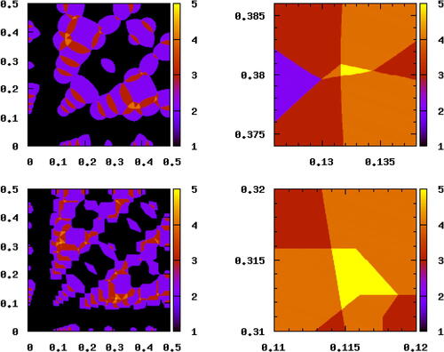
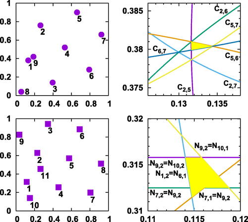
Fig. 4 Upper left: the Kronecker sequence for $\alpha =(0.132,0.38)$, showing five shortest distances in the Euclidean metric, $d_2(\alpha ,9\alpha )<d_2(2\alpha ,9\alpha )<d_2(3\alpha ,9\alpha )<d_2(4\alpha ,9\alpha )<d_2(5\alpha ,7\alpha )$. Upper right: Formation of the curved triangle and other structure in the upper right panel of Figure 3. Here, the two components of α are plotted, with $C_{m,n}$ the circular arc defined by $\mathit{\text{⏧mα⏧}}=\mathit{\text{⏧nα⏧}}$ in the Euclidean metric. Lower left: Kronecker sequence for $\alpha =(0.115,0.314)$ showing the five shortest distances in the maximum metric, $d_{\infty }(\alpha ,11\alpha )<d_{\infty }(2\alpha ,11\alpha )<d_{\infty }(4\alpha ,11\alpha )<d_{\infty }(5\alpha ,11\alpha )<d_{\infty }(6\alpha ,5\alpha )$. Lower right: Formation of the pentagon in the lower right panel of Figure 3. For $N_{n,j}$, see equation (9)(9) $$\mathit{⏧n\alpha }{⏧}_p=\{\begin{array}{cc}{\left(\sum _{j=1}^d{N}_{n,j}^p\right)}^{1/p}& p<\infty \\ {\mathrm{\text{max}}}_{1\le j\le d}{N}_{n,j}& p=\infty \end{array}$$(9) . The boundary of the pentagonal solution set consists of line segments where various combinations of these are equal.

A rational solution with minimal denominator (but not length) is $g_2^2(\alpha ,12)=5$ with $\alpha =(3,8)/29$.

A solution where the region is a (curvilinear) quadrilateral rather than a triangle is $g_2^2(\alpha ,14)=5$ with $\alpha =(0.09,0.381)$ or $\alpha =(5,21)/55$. In this case, the boundary curves are $⏧2\mathit{\alpha ⏧}=⏧8\mathit{\alpha ⏧},⏧3\mathit{\alpha ⏧}=⏧8\mathit{\alpha ⏧},⏧10\alpha =11\mathit{\alpha ⏧},⏧11\alpha =13\mathit{\alpha ⏧}$. So, the longest of the five distances is either $⏧2\mathit{\alpha ⏧}$ or $⏧3\mathit{\alpha ⏧}$ for different parts of the solution region.

3.3 d = 3

The following example is new (though its discovery was noted in Ref. [3]): $g_2^3(\alpha ,58)=9$ with $\alpha =(0.0203,0.0727,0.3853)$ or a close point with minimal denominator $\alpha =\left(\frac{27}{1334},\frac{97}{1334},\frac{514}{1334}\right)$. There are no other (longer) orbits with smaller denominators than this. The descending sequence of norms is $\mathit{⏧n\alpha }{⏧}^2={1334}^{-2}\{128674,128218,125054,104720,95916,92468,91544,88338,81774\}$ with $n=\{13,39,41,42,44,52,54,55,57\}$ and all other norms larger for $1\le n\le 57$. This set of solutions lies in a roughly tetrahedral region of volume close to $4.619\times {10}^{-13}$ bounded by the surfaces $⏧13\mathit{\alpha ⏧}=⏧39\mathit{\alpha ⏧}$, $⏧44\mathit{\alpha ⏧}=⏧52\mathit{\alpha ⏧},⏧52\mathit{\alpha ⏧}=⏧54\mathit{\alpha ⏧}$ and $⏧54\mathit{\alpha ⏧}=⏧55\mathit{\alpha ⏧}$. Symmetry gives $2^{d}d!=48$ copies of this set, so it requires close to 10¹¹ random vectors to find. Note that the upper bound for ${\overline{g}}_2^3$ is ${\sigma }_3+1=13$. However we conjecture that this example is tight, that is, ${\overline{g}}_2^3=9$.

3.4 d = 4

The following example is new: $g_2^4(\alpha ,68)=11$ with $\alpha =(0.0182,0.285725,0.419,0.47625)$. The descending sequence of norms is $\mathit{⏧n\alpha }{⏧}^2={40000}^{-2}\{211374125,209588500,209096500,207136000,204312500,197266000,196599125,193378125,189534125,\mathrm{/}\mathrm{/}181227125,131849125\}$ with $n=\{7,38,46,48,50,52,53,55,57,59,67\}$. The 4-volume of the relevant region is about $3.70\times {10}^{-17}$.

3.5 d = 5

The example is $g_2^5(\alpha ,205)=13$ with $\alpha =(0.10742,0.11374,0.25,0.29918,0.42596)$. The descending sequence is $\mathit{⏧n\alpha }{⏧}^2={10}^{-9}\{162780582,161793408,158326822,158307200,155630688,154482518,154184800,122913878,117497952,117410262,\mathrm{/}\mathrm{/}115212800,85909382,60563808\}$ with $n=\{17,104,113,120,124,131,140,141,148,157,160,167,204\}$. The 5-volume of the relevant region is about $8.42\times {10}^{-21}$. That this region was found within about 10¹² sample size, even taking into account the symmetry factor $5!2^5=3840$ suggests that there are many similar regions.

3.6 d = 6

The random algorithm discovered a solution with $g_2^6(\alpha ,55)=13$, but searching (using a cubic lattice) in the vicinity of this solution improved it to $g_6(\alpha ,55)=14$ with $\alpha =(0.02,0.0715,0.13,0.167,0.2672,0.479)$. The descending sequence is $\mathit{⏧n\alpha }{⏧}^2={10}^{-8}\{35113809,33433369,32828100,32650449,32540196,32494400,30172929,30079076,30014224,27739844,27655936,\mathrm{/}\mathrm{/}25819536,25809481,22827044\}$ with $n=\{1,29,30,31,38,40,41,42,44,46,48,52,53,54\}$. The 6-volume of the relevant region is about $4.2\times {10}^{-23}$.

3.7 Minimal length solutions

We have from equation (15)(15) $$N\ge 2g_p^d-1.$$(15) that $N\ge 2g_2^d-1$. However, the above examples with $d\ge 3$ have much larger N. Table 1 gives examples we have found where this bound is sharp using the exhaustive rational search method with $d\le 6$. It is open whether solutions exist for higher $g_2^d$ than presented here. The example for N = 3 has a shortest distance of zero between the first and third points; if a positive distance is desired, $\alpha =2/5$ provides the minimal denominator example for this case.

Table 1 Examples where the bound equation (15(15) $$N\ge 2g_p^d-1.$$(15) ) is tight for the Euclidean norm.

$g_2^d(\alpha ,N)$	N	α
2	3	1/2
3	5	3/11
4	7	(5, 8)/24
5	9	(15,43)/113
6	11	(24,69,111)/232
7	13	(9,24,29,42)/89
8	15	(12,14,35,57,76)/158

4 Examples for the maximum norm

4.1 d = 1

This case is identical to the Euclidean norm, Section 3.1.

4.2 d = 2

Ref. [4] shows that ${\overline{g}}_{\infty }^2=5$ and gives the solution $\alpha =(0.115,0.314)$ for N = 11. In contrast to the Euclidean case, numerical simulations strongly suggest that this is the minimum N. The maximum norm is in some ways simpler than the Euclidean norm as the solution regions are polytopes; see Figures 3 and 4 which shows a non-convex pentagonal region for this value of N. A rational solution with minimal denominator (at this length) is $$\alpha =\left(\frac{10}{86},\frac{27}{86}\right)=\left(0.1162\dots ,0.3139\dots \right)$$

For this example we find $\mathit{⏧n\alpha }{⏧}_{\infty }={86}^{-1}\{\mathbf{27},32,30,40,37,\mathbf{26},\mathbf{17},42,\mathbf{15},\mathbf{14}\}$ for $1\le n\le 10$ with relevant norms in bold. As with the roughly triangular example in Section 3.2, the boundaries of this region occur where one of the relevant inequalities $\mathit{⏧\alpha }{⏧}_{\infty }>⏧6\alpha {⏧}_{\infty }>⏧7\alpha {⏧}_{\infty }>⏧9\alpha {⏧}_{\infty }>⏧10\alpha {⏧}_{\infty }$ is broken. The maximum norm is, according to equation (9)(9) $$\mathit{⏧n\alpha }{⏧}_p=\{\begin{array}{cc}{\left(\sum _{j=1}^d{N}_{n,j}^p\right)}^{1/p}& p<\infty \\ {\mathrm{\text{max}}}_{1\le j\le d}{N}_{n,j}& p=\infty \end{array}$$(9) , $$\mathit{⏧n\alpha }{⏧}_{\infty }=\mathrm{\text{max}}\left(N_{n,1},N_{n,2}\right)$$

(16) See the lower right panel of Figure 4. The part of the boundary where $⏧9\alpha {⏧}_{\infty }=⏧10\alpha {⏧}_{\infty }$ corresponds to two components, $N_{9,2}=N_{10,2}$ and $N_{9,2}=N_{10,1}$, and similarly $⏧7\alpha {⏧}_{\infty }=⏧9\alpha {⏧}_{\infty }$ corresponds to two components $N_{7,1}=N_{9,2}$ and $N_{7,2}=N_{9,2}$. Finally, the other relevant component is $\mathit{⏧\alpha }{⏧}_{\infty }=⏧6\alpha {⏧}_{\infty }$ corresponding to $N_{1,2}=N_{6,1}$. Unlike the p = 2 norm, each of these components is a straight line segment, yielding exact rational values for the locations of the vertices of the pentagon, clockwise from the upper left: $$\left\{\left(\frac{13}{114},\frac{6}{19}\right),\left(\frac{11}{95},\frac{6}{19}\right),\left(\frac{19}{160},\frac{5}{16}\right),\left(\frac{13}{112},\frac{5}{16}\right),\left(\frac{7}{61},\frac{19}{61}\right)\right\}.$$

The area can be calculated exactly (using Mathematica) to be $$\frac{24863}{2367697920}\approx 1.05\times {10}^{-5}$$

A rational solution with minimal denominator (but not length) is $g_{\infty }^2(\alpha ,14)=5$ with $\alpha =(4,15)/47$.

4.3 d = 3

Ref. [4] shows that ${\overline{g}}_{\infty }^3=9$ and gives a solution equivalent to $g_{\infty }^3(\alpha ,73)=9$ for $\alpha =(0.0157,0.0575,0.23744)$. We have found the slightly simpler solution $g_{\infty }^3(\alpha ,49)=9$ with $\alpha =(0.0824,0.3301,0.4383)$ or with minimal denominator for this length, $$\alpha =\left(\frac{153}{1857},\frac{613}{1857},\frac{814}{1857}\right)=\left(0.08239\dots ,0.33010\dots ,0.43824\dots \right)$$

The descending sequence of norms for the latter is

$\mathit{⏧n\alpha }{⏧}_{\infty }={1857}^{-1}\{480,469,417,415,408,406,396,390,288\}$ with $n=\{9,25,27,34,36,37,39,46,48\}$. The volume of this region is around $2.45\times {10}^{-12}.$

A rational solution with minimal denominator (but not length) is $g_{\infty }^3(\alpha ,181)=9$ with $\alpha =(187,190,203)/468$.

4.4 d = 4

We have the found the following example, of much greater length and distances than others: $g_{\infty }^4(\alpha ,1548)=15$ with $\alpha =$ $(0.14216,0.309579,0.400742,0.42857)$. The descending sequence of norms is $\mathit{⏧n\alpha }{⏧}_{\infty }={10}^{-6}\{143310,141620,141570,141560,$ $141510,141260,141200,141150,129726,121600,97200,90740,83448,81287\}$ with $n=\{317,866,901,908,943,1118,1153,1160,$ $1195,1253,1260,1295,1470,1512,1547\}$. The 4-volume of this region is around $6.5\times {10}^{-21}$.

4.5 Minimal length solutions

As in Section 3.7 we seek solutions where the bound in equation (15)(15) $$N\ge 2g_p^d-1.$$(15) is sharp. For the maximum norm, the example in the proof of Theorem 2 shows that these exist for arbitrary $g_{\infty }^d\le 2^{d-1}+1$. Table 2 gives results from the exhaustive integer search, which suggests that this is close to the best that can be obtained; the examples with $g_{\infty }^d\in \{2,3,4,6\}$ have $g_{\infty }^d>2^{d-1}+1$.

Table 2 Examples where the bound equation (15(15) $$N\ge 2g_p^d-1.$$(15) ) is tight for the maximum norm.

$g_{\infty }^d(\alpha ,N)$	N	α
2	3	1/2
3	5	3/11
4	7	(6, 16)/35
5	9	(5, 10, 17)/36
6	11	(12,35,57)/118
7	13	(9,21,34,39)/80
8	15	(7,23,35,47)/96
9	17	(9,33,52,67)/136
10	19	(11,25,31,47,95)/192
11	21	(13,27,34,55,111)/224
12	23	(15,39,63,95,127)/256
13	25	(19,31,41,79,159)/320
14	27	(41,61,79,89,159)/320

5 Proof of Theorem 1

Proof.

For this theorem, we have p = 2 (Euclidean norm). We verify the examples in Section 3 computationally using exact arithmetic, and apply the result in equation (4)(4) $${\sigma }_d<\frac{d(d-1)2^{d/2}}{(\sqrt{2}-1)\sqrt{\pi }},\mathrm{\hspace{1em}}\mathrm{\hspace{1em}}d\ge 3$$(4) . Mathematica code and an example (d = 3 in the Euclidean metric) are given in Appendix A. □

6 Proof of Theorem 2

For this theorem, we have $p=\infty$ (maximum norm). For d = 4, the example in Section 4.4 is verified using the Mathematica code in Appendix A.

For $d\ge 5$ (and for lower d, but in this case the bound is not optimal) we have the example $\alpha =(1/2^d-ϵ,1/2^{d-1}-ϵ,\dots ,1/2-ϵ)$ with $0<ϵ\le {(2^d(2^d+2))}^{-1}$. In the following, as just before equation (9)(9) $$\mathit{⏧n\alpha }{⏧}_p=\{\begin{array}{cc}{\left(\sum _{j=1}^d{N}_{n,j}^p\right)}^{1/p}& p<\infty \\ {\mathrm{\text{max}}}_{1\le j\le d}{N}_{n,j}& p=\infty \end{array}$$(9) , a subscript indicates vector component. If n is odd, then ${(n\alpha )}_d=1/2-\mathit{nϵ}$. If n is even but not a multiple of 4, then ${(n\alpha )}_{d-1}=1/2-\mathit{nϵ}$ and in general, if n is a multiple of $2^k$ but not $2^{k+1}$ for $0\le k<d$ then the d–k component of $\mathit{n\alpha }$ is $1/2-\mathit{nϵ}$. For ϵ sufficiently small, this will be the component with the largest distance, and hence give the $\infty$-norm. As ϵ is increased, the first violation occurs for $n=2^{d-1}+1$ when ${(n\alpha )}_1=1/2+1/2^d-(2^{d-1}+1)ϵ$ which has norm greater than $1/2-\mathit{nϵ}$ for $ϵ>{(2^d(2^d+2))}^{-1}$, hence the above bound on ϵ. Finally, for $n=2^d$, all components are $-\mathit{nϵ}$. Thus (17) $$\mathit{⏧n\alpha }{⏧}_{\infty }=\{\begin{array}{cc}1/2-\mathit{nϵ}& 1\le n\le 2^d-1\\ \mathit{nϵ}& n=2^d\end{array}$$(17)

which decreases monotonically, and so choosing $N=2^d+1$ gives $2^{d-1}+1$ distances as needed. □

Remark

s:

1. Choosing the maximum value of ϵ gives a rational solution with denominator $2^d(2^d+2)$.

2. Choosing odd $N\le 2^d+1$ gives a solution with $(N+1)/2$ distances, so that equation (15)(15) $$N\ge 2g_p^d-1.$$(15) is sharp.

7 Proof of Lemma 3 and Theorem 4

We use the bound on σ_d given in eq. 2(2) $${\overline{g}}_2^d\ge \{\begin{array}{cc}9& d=3\\ 11& d=4\\ 13& d=5\\ 14& d\ge 6\end{array}$$(2) of Ref. [7], noting that the kissing number corresponds to spherical caps of radius $\alpha =\pi /6$ corresponding to $\beta =\pi /4$ in that paper. (18) $${\sigma }_d\le \frac{\Gamma ((d-1)/2)\sqrt{\pi /8}}{\Gamma (d/2){\int }_0^{\pi /4}{\hspace{0.17em}\mathrm{\text{sin}}\hspace{0.17em}}^{d-2}\theta (\hspace{0.17em}\mathrm{\text{cos}}\hspace{0.17em}\theta -\hspace{0.17em}\mathrm{\text{cos}}\hspace{0.17em}(\pi /4))d\theta },\mathrm{\hspace{1em}}\mathrm{\hspace{1em}}d\ge 2$$(18)

For $d\ge 3$ this can be simplified using $\Gamma ((d-1)/2)<\Gamma (d/2)$ and for $0<\theta <\pi /4$ comparing two concave functions with linear functions between their end points: $\hspace{0.17em}\mathrm{\text{sin}}\hspace{0.17em}\theta >\theta 2\sqrt{2}/\pi$ and $\hspace{0.17em}\mathrm{\text{cos}}\hspace{0.17em}\theta -\hspace{0.17em}\mathrm{\text{cos}}\hspace{0.17em}(\pi /4)>(1-1/\sqrt{2})(1-4\theta /\pi )$. This leads to Lemma 3: (19) $$\begin{array}{c}{\sigma }_d<\frac{\sqrt{\pi /8}}{{\int }_0^{\pi /4}{(\theta 2\sqrt{2}/\pi )}^{d-2}(1-1/\sqrt{2})(1-4\theta /\pi )d\theta }\\ =\frac{d(d-1)2^{d/2}}{(\sqrt{2}-1)\sqrt{\pi }}\equiv R_d,\mathrm{\hspace{1em}}\mathrm{\hspace{1em}}d\ge 3\end{array}$$(19)

Now $R_{21}<2^{20}$ and also $R_{d+1}/R_d=\sqrt{2}(d+1)/(d-1)<2$ for $d\ge 6$. So by induction, $R_d<2^{d-1}$ for all $d\ge 21$. Thus ${\sigma }_d<2^{d-1}$ for all $d\ge 21$. Also, we note that ${\sigma }_d<2^{d-1}$ for $11\le d\le 20$ by known bounds for these dimensions [2, 6].

Thus for all $d\ge 11$ we have ${\overline{g}}_{\infty }^d\ge 2^{d-1}+1>{\sigma }_d+1\ge {\overline{g}}_2^d$ where the first inequality is from Theorem 2 and the last from Ref. [3]. This concludes the proof of Theorem 4. □

8 General p-norms

8.1 d = 1

This case is identical to Section 3.1.

8.2 d = 2: Proof of Theorem 5

We now prove Theorem 5, by giving an example with 5 distances in d = 2, valid for all $p\in [1,\infty ]$.

More precisely, we will show that for all p we can define ${\theta }_{\mathrm{\text{min}}}(p)$ and ${\theta }_{\mathrm{\text{max}}}(p)$ so that when $\theta \in ({\theta }_{\mathrm{\text{min}}}(p),{\theta }_{\mathrm{\text{max}}}(p))$ there exists $ϵ>0$ so that $g_p^2(\alpha ,17)=5$, where α depends on θ and ϵ. Specifically, $\alpha =(6/25+ϵ\hspace{0.17em}\mathrm{\text{cos}}\hspace{0.17em}\theta ,8/25-ϵ\hspace{0.17em}\mathrm{\text{sin}}\hspace{0.17em}\theta ),{\theta }_{\mathrm{\text{min}}}(p)=\mathrm{\text{arctan}}(s)$ and ${\theta }_{\mathrm{\text{max}}}(p)=\mathrm{\text{arctan}}\frac{9+12s}{12-9s}$ where $s={(3/4)}^{p-1}\in [0,1]$. For $p=\infty$, we define these to take their limiting values, namely ${\theta }_{\mathrm{\text{min}}}(\infty )=s=0$ and ${\theta }_{\mathrm{\text{max}}}(\infty )=\mathrm{\text{arctan}}(3/4)$. In all cases $0<\theta <\mathrm{\text{arctan}}(7)<\pi /2$ so $\hspace{0.17em}\mathrm{\text{tan}}\hspace{0.17em}\theta$ is strictly monotonic.

To show that the interval in θ is well defined, note that (20) $$\hspace{0.17em}\mathrm{\text{tan}}\hspace{0.17em}({\theta }_{\mathrm{\text{max}}}(p))-\hspace{0.17em}\mathrm{\text{tan}}\hspace{0.17em}({\theta }_{\mathrm{\text{min}}}(p))=\frac{9(1+s^2)}{12-9s}>0.$$(20)

Now consider $\mathit{n\alpha }$ for $1\le n\le 16$, in particular (21) $$\begin{array}{c}9\alpha =\left(\frac{54}{25}+9ϵ\hspace{0.17em}\mathrm{\text{cos}}\hspace{0.17em}\theta ,\frac{72}{25}-9ϵ\hspace{0.17em}\mathrm{\text{sin}}\hspace{0.17em}\theta \right)\equiv \left(\frac{4}{25}+9ϵ\hspace{0.17em}\mathrm{\text{cos}}\hspace{0.17em}\theta ,-\left(\frac{3}{25}+9ϵ\hspace{0.17em}\mathrm{\text{sin}}\hspace{0.17em}\theta \right)\right)\mathrm{\text{mod }}1\\ 12\alpha =\left(\frac{72}{25}+12ϵ\hspace{0.17em}\mathrm{\text{cos}}\hspace{0.17em}\theta ,\frac{96}{25}-12ϵ\hspace{0.17em}\mathrm{\text{sin}}\hspace{0.17em}\theta \right)\equiv \left(-\left(\frac{3}{25}-12ϵ\hspace{0.17em}\mathrm{\text{cos}}\hspace{0.17em}\theta \right),-\left(\frac{4}{25}+12ϵ\hspace{0.17em}\mathrm{\text{sin}}\hspace{0.17em}\theta \right)\right)\mathrm{\text{mod }}1\\ 13\alpha =\left(\frac{78}{25}+13ϵ\hspace{0.17em}\mathrm{\text{cos}}\hspace{0.17em}\theta ,\frac{104}{25}-13ϵ\hspace{0.17em}\mathrm{\text{sin}}\hspace{0.17em}\theta \right)\equiv \left(\frac{3}{25}+13ϵ\hspace{0.17em}\mathrm{\text{cos}}\hspace{0.17em}\theta ,\frac{3}{25}-13ϵ\hspace{0.17em}\mathrm{\text{sin}}\hspace{0.17em}\theta \right)\mathrm{\text{mod }}1\\ 16\alpha =\left(\frac{96}{25}+16ϵ\hspace{0.17em}\mathrm{\text{cos}}\hspace{0.17em}\theta ,\frac{128}{25}-16ϵ\hspace{0.17em}\mathrm{\text{sin}}\hspace{0.17em}\theta \right)\equiv \left(-\left(\frac{4}{25}-16ϵ\hspace{0.17em}\mathrm{\text{cos}}\hspace{0.17em}\theta \right),\frac{3}{25}-16ϵ\hspace{0.17em}\mathrm{\text{sin}}\hspace{0.17em}\theta \right)\mathrm{\text{mod }}1\end{array}$$(21)

For ϵ = 0 these four p-norms are equal: (22) $$\mathit{⏧n\alpha }{⏧}_p=\{\begin{array}{cc}{\left[{(3/25)}^p+{(4/25)}^p\right]}^{1/p}& p<\infty \\ 4/25& p=\infty \end{array}\mathrm{\hspace{1em}}\mathrm{\hspace{1em}}n\in \{9,12,13,16\},\hspace{1em}ϵ=0.$$(22)

Furthermore, denoting the distance to the nearest integer of the components of $\mathit{n\alpha }$ as $N_{n,j}$ (see equation (9)(9) $$\mathit{⏧n\alpha }{⏧}_p=\{\begin{array}{cc}{\left(\sum _{j=1}^d{N}_{n,j}^p\right)}^{1/p}& p<\infty \\ {\mathrm{\text{max}}}_{1\le j\le d}{N}_{n,j}& p=\infty \end{array}$$(9) ), we note that for n = 1 we have $\mathrm{\text{min}}(N_{1,1},N_{1,2})=6/25>4/25$ and for $2\le n\le 16,n\notin \{9,12,13,16\},\max (N_{n,1},N_{n,2})\ge 3/25+4/25=7/25$ and $\mathrm{\text{min}}(N_{n,1},N_{n,2})>0$. Thus for ϵ = 0 and these n, the p-norm is strictly greater than for $n\in \{9,12,13,16\}$ for all $p\in [1,\infty ]$. This remains true for all sufficiently small positive ϵ.

For small positive ϵ, the $\mathit{⏧n\alpha }{⏧}_p$ for $n\in \{9,12,13,16\}$ will differ, and following the analysis in Section 2, in order to obtain five distances, the minimum distance needs to decrease four times in the range $\frac{N-1}{2}\le n\le N-1$, that is, we need (23) $$⏧9\alpha {⏧}_p>⏧12\alpha {⏧}_p>⏧13\alpha {⏧}_p>⏧16\alpha {⏧}_p$$(23)

Now, we have two cases. First, consider $p<\infty$. For the first inequality we write $⏧9\alpha {⏧}_p^p>⏧12\alpha {⏧}_p^p$ in full, to first order in powers of ϵ: (24) $$\begin{array}{c}{\left(\frac{4}{25}\right)}^p+p{\left(\frac{4}{25}\right)}^{p-1}9ϵ\hspace{0.17em}\mathrm{\text{cos}}\hspace{0.17em}\theta +{\left(\frac{3}{25}\right)}^p+p{\left(\frac{3}{25}\right)}^{p-1}9ϵ\hspace{0.17em}\mathrm{\text{sin}}\hspace{0.17em}\theta \\ >{\left(\frac{3}{25}\right)}^p+p{\left(\frac{3}{25}\right)}^{p-1}(-12)ϵ\hspace{0.17em}\mathrm{\text{cos}}\hspace{0.17em}\theta +{\left(\frac{4}{25}\right)}^p+p{\left(\frac{4}{25}\right)}^{p-1}12ϵ\hspace{0.17em}\mathrm{\text{sin}}\hspace{0.17em}\theta +O({ϵ}^2)\end{array}$$(24)

The constant terms cancel. We divide by $\mathit{pϵ}{(4/25)}^{p-1}$ and neglect higher order terms in ϵ. Also, recall that $s={(3/4)}^{p-1}\in (0,1]$. In this way we obtain (25) $$9\hspace{0.17em}\mathrm{\text{cos}}\hspace{0.17em}\theta +9s\hspace{0.17em}\mathrm{\text{sin}}\hspace{0.17em}\theta >-12s\hspace{0.17em}\mathrm{\text{cos}}\hspace{0.17em}\theta +12\hspace{0.17em}\mathrm{\text{sin}}\hspace{0.17em}\theta$$(25) and hence $\hspace{0.17em}\mathrm{\text{tan}}\hspace{0.17em}\theta <\frac{9+12s}{12-9s}=\hspace{0.17em}\mathrm{\text{tan}}\hspace{0.17em}{\theta }_{\mathrm{\text{max}}}$. By a similar calculation, $⏧12\alpha {⏧}_p>⏧13\alpha {⏧}_p$ is satisfied if $\hspace{0.17em}\mathrm{\text{tan}}\hspace{0.17em}\theta >\hspace{0.17em}\mathrm{\text{tan}}\hspace{0.17em}{\theta }_{\mathrm{\text{min}}}=s$ and $⏧13\alpha {⏧}_p>⏧16\alpha {⏧}_p$ is satisfied if $s\ge 13/16$ or $\hspace{0.17em}\mathrm{\text{tan}}\hspace{0.17em}\theta <\frac{16+13s}{13-16s}$. For this last inequality we have for ${\theta }_{\mathrm{\text{min}}}(p)<\theta <{\theta }_{\mathrm{\text{max}}}(p)$: (26) $$\frac{16+13s}{13-16s}-\hspace{0.17em}\mathrm{\text{tan}}\hspace{0.17em}\theta >\frac{16+13s}{13-16s}-\hspace{0.17em}\mathrm{\text{tan}}\hspace{0.17em}{\theta }_{\mathrm{\text{max}}}=\frac{75-24s+75s^2}{(13-16s)(12-9s)}>0$$(26) since the numerator is positive for all s, and the denominator is also positive when s < 13∕16. Thus, the inequality $⏧13\alpha {⏧}_p>⏧16\alpha {⏧}_p$ is always satisfied when ${\theta }_{\mathrm{\text{min}}}(p)<\theta <{\theta }_{\mathrm{\text{max}}}(p)$.

To summarize, for $\theta \in ({\theta }_{\mathrm{\text{min}}}(p),{\theta }_{\mathrm{\text{max}}}(p))$ the inequalities at first order in ϵ are satisfied, and we can take sufficiently small ϵ to ensure that the higher order terms can be neglected.

The second case is $p=\infty$. Here we can write explicitly that $⏧9\alpha {⏧}_{\infty }=4/25+9ϵ\hspace{0.17em}\mathrm{\text{cos}}\hspace{0.17em}\theta ,⏧12\alpha {⏧}_{\infty }=4/25+12ϵ\hspace{0.17em}\mathrm{\text{sin}}\hspace{0.17em}\theta ,⏧13\alpha {⏧}_{\infty }=4/25-13ϵ\hspace{0.17em}\mathrm{\text{sin}}\hspace{0.17em}\theta$ and $⏧16\alpha {⏧}_{\infty }=4/25-16ϵ\hspace{0.17em}\mathrm{\text{cos}}\hspace{0.17em}\theta$. The inequalities, equation (23)(23) $$⏧9\alpha {⏧}_p>⏧12\alpha {⏧}_p>⏧13\alpha {⏧}_p>⏧16\alpha {⏧}_p$$(23) are satisfied for $0<\hspace{0.17em}\mathrm{\text{tan}}\hspace{0.17em}\theta <3/4$, which is again $\theta \in ({\theta }_{\mathrm{\text{min}}}(p),{\theta }_{\mathrm{\text{max}}}(p))$. □

Remark:

It is an open question whether there are any α and N giving five distances for all p. The above proof shows that solutions are in a small neighborhood of the point $(6/25,8/25)$, but the intervals in θ have no intersection: For p = 1 we need $\hspace{0.17em}\mathrm{\text{tan}}\hspace{0.17em}\theta \in (1,7)$ whilst for $p=\infty$ we need $\hspace{0.17em}\mathrm{\text{tan}}\hspace{0.17em}\theta \in (0,3/4)$.

8.3 d = 3

We have numerical evidence that for all $p\in [1,\infty ]$, there exist α and N such that $g_p^3(\alpha ,N)=9$. Our examples interpolate between the values of p for the four given in Table 3, covering the entire domain in p. The regions in α vary slightly with p.

Table 3 Examples with $g_p^3(\alpha ,N)=9$.

p	N	α
1	148	(0.16915,0.1769,0.2109)
1.3	148	(0.16903,0.177,0.2109)
1.2	124	(0.009,0.06564,0.366233)
2	124	(0.0092,0.06572,0.3662)
1.9	58	(0.02035,0.0727,0.38535)
3	58	(0.0201,0.0728,0.3853)
2.5	94	(0.01217,0.35409,0.409912)
$\infty$	94	(0.0118,0.35395,0.41)

Interpolating these solutions covers all p-norms.

A code to verify solutions

The following Mathematica code was used to verify all the examples given in this paper. Mathematica does arbitrary precision arithmetic and exact comparisons of expressions involving non-integer powers, so it can be used for all values of p, entered as 13/10 rather than 1.3, for example. Following the code, we present the output for three examples, found in sections 3.3, 4.4 and 8.3. Equivalent code can be written in computer languages using fixed precision integers for integer or infinite p, and denominators not too large.

Mathematica 11.0.1 for Linux x86 (64-bit)

Copyright 1988-2016 Wolfram Research, Inc.

In[1]:=! cat dists.m

Print["p-metric distances for exact p> =1 or Infinity"]

qreduce[a_,q_]:=Abs[a-q*Floor[a/q + 0.5]]

distlist[alist_,q_,Nmax_]:=If[p==Infinity,

Table[Max[Table[qreduce[n*alist[[i]],q],{i,Length[alist]}]],{n,Nmax}],

Table[Sum[qreduce[n*alist[[i]],q]^p,{i,Length[alist]}],{n,Nmax}]]

dists[alist_,q_,Nmax_]:=(Print["p="< >ToString[p]< >", N="< >ToString[Nmax]< >","];/

Print["alpha="< >ToString[alist]< >"/"< >ToString[q]];/

dl = distlist[alist,q,Nmax];min = Infinity;count = 1;/

For[i = 1,i< =Nmax-1,i++,If[dl[[i]]<min,min = dl[[i]];/

Print[ToString[i]< >" "< >ToString[InputForm[dl[[i]]]]];If[i > Nmax/2,count++]]];/

Print["Distances="< >ToString[count]])

In[2]:= ≪ dists.m

p-metric distances for exact p> =1 or Infinity

In[3]:= p = 2

Out[3] = 2

In[4]:= dists[{27,97,514},1334,58]

p = 2, N = 58,

alpha = {27, 97, 514}/1334

1 274334

2 134188

13 128674

39 128218

41 125054

42 104720

44 95916

52 92468

54 91544

55 88338

57 81774

Distances = 9

In[5]:= p = Infinity

Out[5]= Infinity

In[6]:= dists[{142160,309579,400742,428570},1000000,1548]

p = Infinity, N = 1548,

alpha = {142160, 309579, 400742, 428570}/1000000

1 428570

2 380842

7 194806

35 164735

77 162417

210 155820

317 143310

866 141620

901 141570

908 141560

943 141510

1118 141260

1153 141210

1160 141200

1195 141150

1253 129726

1260 121600

1295 97200

1470 90740

1512 83448

1547 81287

Distances = 15

In[7]:= p = 13/10

13

Out[7]=–

10

In[8]:= dists[{16903,17700,21090},100000,148]

p = 13

–

10, N = 148,

alpha = {16903, 17700, 21090}/100000

1 17700*10^(3/5)*177^(3/10) + 16903*16903^(3/10) + 21090*21090^(3/10)

5 11500*2^(3/5)*5^(9/10)*23^(3/10) + 5450*5^(3/5)*218^(3/10) + 15485*15485^(3/10)

90 7000*7^(3/10)*10^(9/10) + 1900*10^(3/5)*19^(3/10) + 21270*21270^(3/10)

95 18500*2^(3/5)*5^(9/10)*37^(3/10) + 3550*5^(3/5)*142^(3/10) + 5785*5785^(3/10)

113 100*10^(3/5) + 16830*3^(3/5)*1870^(3/10) + 10039*10039^(3/10)

118 11400*2^(9/10)*5^(3/5)*57^(3/10) + 11380*2^(3/5)*2845^(3/10) + 5446*5446^(3/10)

119 6300*7^(3/10)*30^(3/5) + 11457*3^(3/5)*1273^(3/10) + 9710*9710^(3/10)

124 10400*2^(1/5)*5^(3/5)*13^(3/10) + 4028*2^(3/5)*1007^(3/10) + 15160*2^(9/10)*1895^(3/10)

142 13400*2^(9/10)*5^(3/5)*67^(3/10) + 5220*6^(3/5)*145^(3/10) + 226*226^(3/10)

147 1900*10^(3/5)*19^(3/10) + 230*230^(3/10) + 15259*15259^(3/10)

Distances = 9

Acknowledgments

The author thanks Mark Pearson for extending the code for uniform random search to GPU processors, and running it. This led to the solutions for p = 2 and $4\le d\le 6$ presented here. The author also thanks Alon Agin, Henry Cohn, Alan Haynes, and Jens Marklof for helpful discussions. This work was carried out using the computational facilities of the Advanced Computing Research Center, University of Bristol—http://www.bristol.ac.uk/acrc/

Declaration of interests

No potential competing interest was reported by the author.

References

- Biringer, I., Schmidt, B. (2008). The three gap theorem and Riemannian geometry. Geom. Dedicata 136: 175–190. 10.1007/s10711-008-9283-8
- de Laat, D., Leijenhorst, N. (2022). Solving clustered low-rank semidefinite programs arising from polynomial optimization. ArXiv preprint arXiv:2202.12077.
- Haynes, A., Marklof, J. (2022). A five distance theorem for Kronecker sequences. Int. Math. Res. Not. 2022(24): 19747–19789. 10.1093/imrn/rnab205
- Haynes, A., Ramirez, J. J. (2021). Higher-dimensional gap theorems for the maximum metric. Int. J. Number Theory 17: 1665–1670. 10.1142/S1793042121500548
- Kellendonk, J., Lenz, D., Savinien, J. (2015). Mathematics of Aperiodic Order, Vol. 309. Basel: Springer.
- Machado, F. C., de Oliveira Filho, F. M. (2018). Improving the semidefinite programming bound for the kissing number by exploiting polynomial symmetry. Exp. Math. 27: 362–369. 10.1080/10586458.2017.1286273
- Rankin, R. A. (1955). The closest packing of spherical caps in n dimensions. Glasgow Math. J. 2: 139–144. 10.1017/S2040618500033219
- Sós, V. T. (1957). On the theory of Diophantine approximations. I 1 (on a problem of A. Ostrowski). Acta Math. Hungarica 8: 461–472. 10.1007/BF02020329
- Sós, V. T. (1958). On the distribution mod 1 of the sequence nα. Ann. Univ. Sci. Budapest, Eötvös Sect. Math. 1: 127–134.
- Świerczkowski, S. (1958). On successive settings of an arc on the circumference of a circle. Fundamenta Math. 46: 187–189. 10.4064/fm-46-2-187-189
- Weiß, C. (2022). Multi-dimensional Kronecker sequences with a small number of gap lengths. Discrete Math. Appl. 32: 69–74. 10.1515/dma-2022-0006