A spatial epidemic model with contact and mobility restrictions

ABSTRACT

Several spatiotemporal epidemic models have described how contact and mobility restrictions have a dynamic effect on morbidity and mortality of fast transmitting pathogens in epidemics. Despite this, there have been rather limited contributions looking at policy optimization. This work combines a new spatiotemporal epidemic model of a heterogeneous mixed population located at different places with an optimal control approach to show the effects of contact and mobility restrictions under policy optimization. The objective of optimization not only includes epidemiological but also socio-economic implications of the restrictions. Several scenarios are numerically investigated, and the dependence of the optimal policy on some basic epidemiological parameters is analysed. The results illustrate the strong impact of spatial heterogeneity on optimal policy measures. An analysis of the stability of the disease-free equilibrium of the model is also presented.

KEYWORDS:

• Infectious diseases
• spatial epidemic model
• optimal policy

1. Introduction

Considering spatially heterogeneous mixing and interventions in infectious disease epidemiological modelling is essential. Human mobility and its effects on contact patterns geographically play a key role in the transmission of pathogens to humans, especially in the case of airborne infectious pathogens such as influenza and corona viruses. The general concepts in heterogeneity of host population in epidemic models have been described in the literature (Hethcote 1996; Brauer et al. 2019) with further developed concepts that include mobility and indirect transmission (Castillo-Chavez et al. 2016; David et al. 2020).

One way to model human mobility with heterogeneous mixing and the impact on airborne pathogen transmission is to divide the population into subgroups with different activity levels. David and Iyaniwura (2022) consider a Susceptible-Infected-Removed (SIR)-type model at each place of residence and use a coupled partial differential equation (PDE)-ordinary differential equations (ODE) system to study the effects of human mobility on airborne pathogen transmission in a heterogeneously mixed population setting. By doing so, they can track the epidemic development at an individual’s place of residence at any time. The corresponding transmission mechanism of the pathogen is diffusion. The authors obtain a flattening epidemic curve as the diffusion rate of the pathogen increases. Zhang and Jin (2022) introduce a model with two geographical areas interconnected due to travel between the areas. The reproduction numbers and the final state of the disease are investigated depending on the contact rate and probability of early diagnostics. Bertaglia et al. (2021) develop a spatial multiscale model with transport of commuters and diffusion of non-commuters in urban areas using data from Italy.

With a reaction – diffusion system Chen et al. (2021) define distance based on the mobility network among various locations. In the network the weights of the edges between pairs of locations are the relative population flow among them. The authors select sub-regions in epidemic areas with active population movements and derive solutions to initiate new travel flows among the sub-regions. Applying their approach to Corona Virus Disease of 2019 (COVID-19) they find that lifting travel restrictions based on their solutions will not cause a new epidemic wave. Geng et al. (2020) use a kernel-modulated SIR modelling approach to characterize the dynamic of Severe Acute Respiratory Syndrome Coronavirus (SARS-CoV-2) in a multifractal distributed susceptible population. The model reproduced multiphase COVID-19 epidemics and explained the fact that while the reproduction number was reduced due to interventions such as social distancing, subsequent epidemic waves still occurred. This was attributed to an increase in susceptible population flow following a relaxation of travel restrictions. Grimee et al. (2021) use a spatiotemporal extension of a multivariate time series model that additively decomposes incidence into an endemic and an epidemic component. The epidemic component captures incidence driven by previous case counts, and the endemic component captures exogenous contributions to incidence such as seasonal factors. Spatial dependencies are captured by neighbourhood matrices adjusted over time to reflect changes in spatial connectivity between geographical areas. The approach applied to COVID-19 with data and indicators describing mobility patterns and travel restrictions. Scenarios of border closures and their effects on the number of cases were studied.

Meta-population dynamical models have also been used to capture the spatiotemporal transmission of SARS-CoV-2. Aguilar et al. (2022) employed a meta-population framework to show the role of urban flows in infectious disease spreading. They find that cities where flows are between hotspots show high vulnerability to the rapid spread of the pathogen with mobility restrictions to be effective in controlling the epidemic. Sprawled cities show a slower spread of the pathogens but with a weaker effect of mobility restrictions such as population travel. In an application in China provinces the spatial diffusion of the infection was captured by parameterizing human mobility Jia et al. (2022). Rapti et al. (2023) developed also a meta-population model incorporating mobility across the province nodes of Andalusia in Spain using mobile-phone time-dependent data. Mazzoli et al. (2021) looked within a similar meta-population framework at the contribution of multi-seeding in association with mobility and lock-downs and how they affect the local transmission of SARS-CoV-2. In a meta-population model based on temporal networks Parino et al. (2021) use COVID-19 data in Italy to investigate reduced social activity and mobility restrictions. They show that the effects of mobility restrictions strongly depend on timely contact and mobility restrictions in the early phases of the outbreak. They argue in favour of social activity reduction policies afterwards. In a geo-hierarchical model Topirceanou and Precup (2021) incorporate the spatial distribution of hierarchically structured population into geographical settlements. They model the movement of individuals using travel distance and frequency parameters for inter- and intra-settlement movement. Their SIR type model reproduces high variation in size and temporal heterogeneity. Epidemic size was more sensitive to increased distance of travel than frequency of travelling. Schoot Uiterkamp et al. (2022) investigated under which epidemiological conditions incorporating mobility into transmission models improves forecasting. The authors utilized a simple mobility-enhanced SEIR compartmental model with commuter information at the municipality level. Inter-regional mobility consideration generally led to an improvement in forecast quality. When policies were in place that aimed to reduce contacts or travel, this improvement was very small. The improvement became larger when municipalities had a relatively large amount of incoming mobility compared with the number of inhabitants.

In an epidemic model Nakata and Roest (2015) describe the effects of transportation networks consisting of heterogeneous regions on pathogen transmission during transportation. Using stability theory of delay differential equations, theory of asymptotically autonomous semiflows and cooperative sublinear dynamical systems, they show that for weakly connected transportation networks endemic patterns exist with a globally asymptotically stable equilibrium, which may be disease-free in some regions while endemic in other regions. Spatial heterogeneity with different basic reproduction numbers they may depend non-monotonically on the dispersal rates indication that travel restrictions may not always be beneficial.

Arino and Van Den Driessche (2023) consider a multi-city epidemic model similar to the one in the present paper, for which conditions for stability of the disease-free population and the basic reproduction rate are obtained and illustrative numerical simulations are given. The model in Zakary et al. (2016) is also similar and contains control variables, but has the substantial difference that the removal is complete and permanent (both after infection or due to an ‘awareness program’).

In many of these studies the effects of control strategies were investigated, but no policy optimization was attempted (except Zakary et al. (2016)). This is also a general observation in the corresponding literature on the spread of epidemics in space.

The aim of this work is to study policy strategies for the control of epidemics and in particular fast unfolding outbreaks of aerially transmitted pathogens such as SARS-CoV-2 or influenza, taking into account the geographical spread of the disease. The experience with the early COVID-19 spread in Austria, Italy, and many other countries shows the role of size, economic activities and peoples mobility for the geographical spread of the epidemic. Adequate early regional policy measures have the potential to slow down the size of the disease and avoid over-occupancy of hospitals, hence, to reduce lethality. The latter is the primary goal of decision makers in the health care sector. On the other hand, the direct and indirect costs related to policy measures such as contact restrictions and lock-downs, and also their social consequences, should be regarded at political level. We do this in the present paper, proposing and analysing a model that incorporates geographical aspects of an epidemic and involves optimization of the above mentioned policy measures. In that we build on existing SIR-type models on graphs (see the literature review above) and on works taking into account the economic losses and social disutility caused by policy measures, e.g. Bloom, Kuhn and Prettner Bloom et al. (2020), Caulkins et al. (2021). Although the optimal policies are numerically obtained by applying optimal control theory in continuous time, therefore are not practically implementable, they may give to the decision-maker useful qualitative information and hints.

The main new features of the presented model and analysis are as follows: (i) we include the three main preventive policy measures – contact rate reduction, lock-downs, and testing; (ii) we consider optimal policies taking into account the number of deaths, economic consequences, and social disutility, and investigate how the weights attributed to these criteria in a common objective functional affects the optimal polices.

The paper is structured as follows: In section 2 we describe the SIR type model with its spatial characteristics assuming proportional random mixing of the population. In addition, we extend the model and introduce two types of control policies. First, we look at the effects of contact restrictions at place $\mathit{x}$ that do not affect business continuity. Second, we explore the scenario of mobility restriction, e.g. travelling from place $\mathit{x}$ to place $\mathit{y}$ having consequences for the business activity. In section 3 we perform a stability analysis of the disease-free equilibrium and calculate the basic reproduction number. The optimization of the policy measures towards minimization of the number of deaths, under explicit consideration of the socio-economic costs caused by the policy measures, is presented in section 4. Corresponding numerical results and analysis of the dependence of the optimal policy and the evolution of the epidemic on some basic model parameters are given in section 5. In section 6 we provide a discussion of the results also in the sense of potential implications for policy making.

2. The basic model and its control extension

We consider a geographical region $\mathrm{\Omega }$ consisting of $\mathit{M}$ cities (further called locations), denoted by $x_1,\dots ,x_M$. The population at each location consists of three groups: $\mathit{S}(\mathit{t},\mathit{x})$ is the size of the susceptible population at location $\mathit{x}\in \mathrm{\Omega }$ and time $\mathit{t}$; $\mathit{I}(\mathit{t},\mathit{x})$ and $\mathit{R}(\mathit{t};\mathit{x})$ are the respective sizes of the infected and the recovered subpopulations. The model presented in this section is a spatial extension of the usual SIR epidemiological model¹; it is purely descriptive and does not essentially differ from other multi-city models (e.g. (Arino and Van Den Driessche 2023)) except in the parametrization, which allows to involve control actions in the next section. The main parameters of the model are:

$\mathit{\iota }$ – force of infection,

$\mathit{\rho }$ – recovery rate,

$\mathit{\nu }$ – rate of transition from recovered to susceptible due to waning immunity,

$\mathit{\mu }$ – mortality rate due to disease,

$\mathit{c}(\mathit{t},\mathit{x})$ – contact rate at location $\mathit{x}$ (the dependence on $\mathit{t}$ may account for seasonal changes),

$\mathit{\alpha }(\mathit{t})$ – fraction of the infected individuals participating in contacts (activity rate of infected),

$\mathit{\sigma }(\mathit{x},\mathit{y})$ – fraction of residents of location $\mathit{x}$ who visit location $\mathit{y}\in \mathrm{\Omega }$ per unit of time.

‘Visits’ may be due to work, shopping, tourism, etc. The parameter $\mathit{\sigma }(\mathit{x},\mathit{y})$ should take into account the time that residents of $\mathit{x}$ spend at $\mathit{y}$. If a ‘Visits’ from $\mathit{x}$ to $\mathit{y}$ is due to work, then only about a half of the (active) time is spent at $\mathit{y}$, the other half is spent at $\mathit{x}$. If a visit is for shopping, for example, then only a smaller fraction of the time is spent at $\mathit{y}$. If a visit is for vacation, then all the time is spent at $\mathit{y}$. Thus, $\mathit{\sigma }(\mathit{x},\mathit{y})$ should not just reflect the number of visits from $\mathit{x}$ to $\mathit{y}$ per day; all the above information has to be incorporated in the parameter $\mathit{\sigma }$. Of course, ${\sum }_{\mathit{y}\in \mathrm{\Omega }}\mathit{\sigma }(\mathit{x},\mathit{y})=1$ for every $\mathit{x}$. Realistically, $\mathit{\sigma }(\mathit{x},\mathit{y})$ is time-dependent due to usual touristic, agricultural, and other activities that are seasonal. However, if the model is used for short-term predictions/control, the mobility (and other) data can be regarded as time-invariant.

The following comment concerns the parameter $\mathit{\alpha }$. The participation of infected individuals in contacts critically depends on whether the individuals know that they are infected. This especially applies to infections with a relatively long asymptomatic period. However, in the model we do not distinguish between asymptomatic and symptomatic infected individuals. Therefore, $\mathit{\alpha }$ represents the overall participation of asymptomatic and symptomatic individuals. Notice that $\mathit{\alpha }(\mathit{t})$ may be influenced by testing, which allows infected people to reduce their contacts before appearance of symptoms, hence to decrease $\mathit{\alpha }$. For this reason, we allow dependence of $\mathit{\alpha }$ on time. We mention that a more precise account of the dependence of the model parameters, in particular $\mathit{\alpha }$, on the phase of infection involves the time since infection as an additional parameter of heterogeneity, see e.g. Kovacevic et al. (2022).

Similarly as in the SIR model, the dynamics of the epidemics on a time interval $[0,\mathit{T}]$ is described by the equations

(2.1). $\frac{\mathrm{d}}{\mathrm{d}t}\mathit{S}(\mathit{t},\mathit{x})=-\sum _{\mathit{y}\in \mathrm{\Omega }}\mathit{c}(\mathit{t},\mathit{y})\mathit{D}(\mathit{t},\mathit{y})\mathit{\sigma }(\mathit{x},\mathit{y})\mathit{S}(\mathit{t},\mathit{x})+\mathit{\nu R}(\mathit{t},\mathit{x}),\mathit{S}(0,\mathit{x})=S_0(\mathit{x}),$(2.1).

(2.2) $\frac{\mathrm{d}}{\mathrm{d}\mathit{t}}\mathit{I}(\mathit{t},\mathit{x})=\sum _{\mathit{y}\in \mathrm{\Omega }}\mathit{c}(\mathit{t},\mathit{y})\mathit{D}(\mathit{t},\mathit{y})\mathit{\sigma }(\mathit{x},\mathit{y})\mathit{S}(\mathit{t},\mathit{x})-(\mathit{\rho }+\mathit{\mu })\mathit{I}(\mathit{t},\mathit{x}),\mathit{I}(0,\mathit{x})=I_0(\mathit{x}),$(2.2)

(2.3) $\frac{\mathrm{d}}{\mathrm{d}\mathit{t}}\mathit{R}(\mathit{t},\mathit{x})=-\mathit{\nu R}(\mathit{t},\mathit{x})+\mathit{\rho I}(\mathit{t},\mathit{x}),\mathit{R}(0,\mathit{x})=R_0(\mathit{x}),$(2.3)

with $\mathit{t}\in [0,\mathit{T}]$, $\mathit{x}\in \mathrm{\Omega }$, where $\mathit{D}(\mathit{t},\mathit{y})$ is the infectiousness (risk of getting infected) at locations $\mathit{y}$. Assuming proportional random mixing it takes the form

(2.4.) $\mathit{D}(\mathit{t},\mathit{y})=\mathit{\iota }\frac{{\sum }_{\mathit{z}\in \mathrm{\Omega }}\mathit{\sigma }(\mathit{z},\mathit{y})\mathit{\alpha }(\mathit{t})\mathit{I}(\mathit{t},\mathit{z})}{{\sum }_{\mathit{z}\in \mathrm{\Omega }}\mathit{\sigma }(\mathit{z},\mathit{y})(\mathit{S}(\mathit{t},\mathit{z})+\mathit{R}(\mathit{t},\mathit{z})+\mathit{\alpha }(\mathit{t},\mathit{z})\mathit{I}(\mathit{t},\mathit{z}))}.$(2.4.)

We mention that in the above model the spatial spread of the infection is entirely and explicitly driven by travel intensities, $\mathit{\sigma }(\mathit{x},\mathit{y})$; no continuous spatial diffusion is involved, which may be reasonable in regions with relatively homogeneous population distribution, see e.g Bertaglia et al. (2021). Demographic aspects are also not considered, assuming stationary reproduction of the disease-free population. Clearly, additional compartments of infected individuals can be considered within the same model, such as asymptomatic isolated/non-isolated, symptomatic, hospitalized, etc., which we do not do in order to keep the model structurally simple.

The model can be extended by introducing two types of policies (in addition to $\mathit{\alpha }$, which will only be used for comparative analysis). The first one, denoted by $\mathit{u}(\mathit{t},\mathit{x})\in [u_0,1]$, is a restriction of the contacts at place $\mathit{x}$ without affecting the business activities. It may take the form of various policies of wearing masks, restrictions for visiting public places, physical distancing, etc. A value $\mathit{u}(\mathit{t},\mathit{x})<1$ means reduction of the contacts to a fraction $\mathit{u}(\mathit{t},\mathit{x})$ of the normal ones. In contrast, a second policy variable, $\mathit{v}(\mathit{t},\mathit{y})\in [v_0,1]$, restricts the business activities at $\mathit{y}$ to a fraction $\mathit{v}(\mathit{t},\mathit{y})$ of the normal one. As a result, also the travel intensity to $\mathit{y}$ reduces by the same fraction, therefore we identify this restriction with travel (mobility) restriction. For example, if factories at $\mathit{y}$ close then commuting for work to $\mathit{y}$ will be reduced; if hotels at a touristic location close then touristic visits to $\mathit{y}$ will reduce proportionally, etc. As a result of the travelling restrictions, an additional fraction $(1-\mathit{v}(\mathit{t},\mathit{y}))\mathit{\sigma }(\mathit{x},\mathit{y})$ of residents of $\mathit{x}$ visiting $\mathit{y}$ (in case of no restrictions) will stay at $\mathit{x}$. We also mention that the control $\mathit{v}(\mathit{t},\mathit{y})$ restricts entering location $\mathit{y}$ but not leaving it. The latter kind of restrictions can also be easily modelled, which is not done in this paper.

In summary, we have the following control variables on a given time-interval $[0,\mathit{T}]$:

• Contact (social) restrictions at $\mathit{x}$ : $\mathit{u}(\mathit{t},\mathit{x})$, with $\mathit{u}:[0,\mathit{T}]\times \mathrm{\Omega }\to [u_0,1]$, where $0<u_0<1$;

• Partial lock-down at $\mathit{y}$ (which leads to less travel to $\mathit{y}$ for work, touristic/vacation visits, shopping, etc.): $\mathit{v}(\mathit{t},\mathit{y})$, with $\mathit{v}:[0,\mathit{T}]\times \mathrm{\Omega }\to [0,1]$.

Having in mind the mobility restrictions $\mathit{v}(\mathit{t},\mathit{x})$ we define the modified mobility function

$\mathit{\psi }(\mathit{t},\mathit{x},\mathit{y}):=\left\{\begin{array}{cc}\mathit{v}(\mathit{t},\mathit{y})\mathit{\sigma }(\mathit{x},\mathit{y})& \mathrm{for}\mathrm{y}\mathit{/}=\mathrm{x},\\ \mathit{v}(\mathit{t},\mathit{x})\mathit{\sigma }(\mathit{x},\mathit{x})+\mathit{\beta }{\sum }_{\mathit{\xi }\in \mathrm{\Omega }}(1-\mathit{v}(\mathit{t},\mathit{\xi }))\mathit{\sigma }(\mathit{x},\mathit{\xi })& \mathrm{for}\mathit{y}=\mathit{x}.,\end{array}\right.$

which is the fraction of residents of $\mathit{x}$ visiting $\mathit{y}$, given the lock-down policy $\mathit{v}(\mathit{t},\cdot )$. Thus, the value $\mathit{\psi }(\mathit{t},\mathit{x},\mathit{y})$ has to replace $\mathit{\sigma }(\mathit{x},\mathit{y})$ in (2.1), (2.2) and (2.4). Moreover, we abbreviate $\mathit{E}(\mathit{t},\mathit{x})=(\mathit{S}(\mathit{t},\mathit{x}),\mathit{I}(\mathit{t},\mathit{x}),\mathit{R}(\mathit{t},\mathit{x}))$. The overall controlled epidemic dynamics takes the form

(2.5) $\frac{\mathrm{d}}{dt}\mathit{S}(\mathit{t},\mathit{x})=-\mathit{G}(\mathit{t},\mathit{x},\mathit{E}(\mathit{t},\cdot ))\mathit{S}(\mathit{t},\mathit{x})+\mathit{\nu R}(\mathit{t},\mathit{x}),$(2.5)

(2.6) $\frac{\mathrm{d}}{\mathrm{d}\mathrm{t}}\mathit{I}(\mathit{t},\mathit{x})=\mathit{G}(\mathit{t},\mathit{x},\mathit{E}(\mathit{t},\cdot ))\mathit{S}(\mathit{t},\mathit{x})-(\mathit{\rho }+\mathit{\mu })\mathit{I}(\mathit{t},\mathit{x}),$(2.6)

(2.7) $\frac{\mathrm{d}}{\mathrm{d}\mathrm{t}}\mathit{R}(\mathit{t},\mathit{x})=-\mathit{\nu R}(\mathit{t},\mathit{x})+\mathit{\rho I}(\mathit{t},\mathit{x}).$(2.7)

where

$\mathit{G}(\mathit{t},\mathit{x},\mathit{E}(\mathit{t},\cdot )):=\sum _{\mathit{y}\in \mathrm{\Omega }}\mathit{u}(\mathit{t},\mathit{y})\mathit{c}(\mathit{t},\mathit{y})\mathit{D}(\mathit{t},\mathit{y},\mathit{E}(\mathit{t},\cdot ))\mathit{\psi }(\mathit{t},\mathit{x},\mathit{y}),$

and

$\mathit{D}(\mathit{t},\mathit{y},\mathit{E}(\mathit{t},\cdot )):=\mathit{\iota \alpha }(\mathit{t})\frac{{\sum }_{\mathit{z}\in \mathrm{\Omega }}\mathit{\psi }(\mathit{t},\mathit{z},\mathit{y})\mathit{I}(\mathit{t},\mathit{z})}{{\sum }_{\mathit{z}\in \mathrm{\Omega }}\mathit{\psi }(\mathit{t},\mathit{z},\mathit{y})(\mathit{S}(\mathit{t},\mathit{z})+\mathit{R}(\mathit{t},\mathit{z})+\mathit{\alpha }(\mathit{t})\mathit{I}(\mathit{t},\mathit{z}))}.$

Although the functions $\mathit{D}$ and $\mathit{G}$ depend on the time $\mathit{t}$, sometimes we suppress $\mathit{t}$ in the notations. Similarly, $\mathit{\psi }(\mathit{t},\mathit{x},\mathit{y})$ depends on $\mathit{v}(\mathit{t},\mathit{y})$, thus $\mathit{D}$ depends on $\mathit{v}(\mathit{t},\cdot )$, $\mathit{G}$ depends on $\mathit{v}(\mathit{t},\cdot )$ and $\mathit{u}(\mathit{t},\cdot )$, which are not explicit in the notations.

Throughout the paper, we assume that the data listed at the beginning of Section 2 are nonnegative and continuous in $\mathit{t}$, the components of $\mathit{E}(0,\mathit{x})$ are nonnegative, $\mathit{S}(0,\mathit{x})+\mathit{I}(0,\mathit{x})+\mathit{R}(0,\mathit{x})>0$ for each $\mathit{x}\in \mathrm{\Omega }$.

3. Stability of the disease-free equilibrium and basic reproduction numbers

To investigate the stability of the disease-free equilibrium, we assume that all data $\mathit{c}(\mathit{x})$, $\mathit{\sigma }(\mathit{x},\mathit{y})$, $\mathit{u}(\mathit{x})$, $\mathit{v}(\mathit{x})$, $\mathit{\alpha }$, with $\mathit{x},\mathit{y}\in \mathrm{\Omega }$, are time-invariant. Also assume that the initial $E_0:=(S_0,0,R_0)$ is disease-free ($R_0$ is considered as [temporarily, if $\mathit{\nu }>0$] ‘protected’ sub-population).

The Jacobian of the right – hand side of (2.5)– (2.7) at $E_0$, denoted further by $\mathit{J}$, is a $(3\mathit{M}\times 3\mathit{M})$-matrix. Obviously $\mathit{D}(\mathit{y},E_0(\cdot ))=0$, hence $\mathit{G}(\mathit{x},E_0(\cdot ))=0$ for all $\mathit{x},\mathit{y}\in \mathrm{\Omega }$. By a direct calculation, we see that

$\frac{\mathrm{\partial }D(x_j,\mathit{E}(\cdot ))}{\mathrm{\partial S}(x_k)}{}_{|E=E_0}=0,\mathrm{hence}\frac{\mathrm{\partial }G(x_i,\mathit{E}(\cdot ))}{\mathrm{\partial S}(x_j)}{}_{|E=E_0}=0,\mathit{i},\mathit{j},\mathit{k}\in \{1,\dots ,\mathit{M}\}.$

Moreover, the right-side of (2.7) is independent of $\mathit{S}$. Hence, the first $\mathit{M}$ columns of $\mathit{J}$ are zero. In addition, similarly as above

$\frac{\mathrm{\partial }G(x_i,\mathit{E}(\cdot ))}{\mathrm{\partial R}(x_j)}{}_{|E=E_0}=0,\mathit{i},\mathit{j}\in \{1,\dots ,\mathit{M}\}.$

Thus, the matrix $\mathit{J}$ has the following structure:

(3.1) $\mathit{J}=\left(\begin{array}{cccc}0& \mathit{P}& \mathit{\nu }\mathcal{I}& \mathit{\hspace{0.17em}}\\ 0& \mathit{J}& 0& \mathit{\hspace{0.17em}}\\ 0& \mathit{\rho I}& -\mathit{\nu }\mathcal{I}& \mathit{\hspace{0.17em}}\end{array}\right),$(3.1)

where $\mathit{I}$ is the identity matrix of dimension $\mathit{M}$, $\mathit{P}$ is matrix of no interest, $\mathit{J}$ has components

$\frac{\mathrm{\partial }(G(x_i,\mathit{E}(\cdot ))\mathit{S}(x_i)-(\mathit{\rho }+\mathit{\mu })\mathit{I}(x_i))}{\mathrm{\partial I}(x_j)}{}_{|E=E_0}.$

One can express

$\frac{\mathrm{\partial }G(x_i,\mathit{E}(\cdot ))}{\mathrm{\partial I}(x_j)}{}_{|E=E_0}=\sum _{\mathit{k}=1}^M\mathit{u}(x_k)\mathit{c}(x_k)\frac{\mathrm{\partial }D(x_k,E_0(\cdot ))}{\mathrm{\partial I}(x_j)}\mathit{\psi }(x_i,x_k),$

and

$\frac{\mathrm{\partial }D(x_k,\mathit{E}(\cdot ))}{\mathrm{\partial I}(x_j)}{}_{|E=E_0}=\mathit{\iota \alpha }\frac{\psi (x_j,x_k)}{\mathit{B}(x_k)},\mathrm{where}\mathit{B}(x_k):=\sum _{\mathit{s}=1}^M\mathit{\psi }(x_s,x_k)(S_0(x_s)+R_0(x_s)).$

Hence,

$\mathit{J}=\mathit{A}-(\mathit{\rho }+\mathit{\mu })\mathcal{I},$

where $\mathit{A}$ has the entries

(3.2) $a_{\mathit{ij}}:=\mathit{\iota \alpha }\sum _{\mathit{k}=1}^M\mathit{u}(x_k)\mathit{c}(x_k)\frac{\psi (x_j,x_k)}{\mathit{B}(x_k)}\mathit{\psi }(x_i,x_k)S_0(x_i),\mathit{i},\mathit{j}\in \{1,\dots ,\mathit{M}\}.$(3.2)

Having in mind (3.1) we obtain that $\mathit{J}$ has $\mathit{M}$ eigenvalues equal to zero (corresponding to the $\mathit{S}$-variables), $\mathit{M}$ eigenvalues equal to $-\mathit{\nu }$ (corresponding to the $\mathit{R}$-variables), and the other $\mathit{M}$ are the eigenvalues of $\mathit{J}$.

Lemma 3.1.

All eigenvalues of the matrix $\mathit{A}$ are real.

Proof.

Denote $b_{\mathit{ij}}$ the same expressions as for $a_{\mathit{ij}}$ with removed $S_0(x_i)$, that is, $a_{\mathit{ij}}=b_{\mathit{ij}}{S}_0(x_i)$, and by $\mathit{B}$ the matrix with entries $b_{\mathit{ij}}$. From its definition, $\mathit{B}$ is a symmetric matrix. Denote by $\mathit{C}$ the diagonal matrix with entries $\sqrt{S_0(x_1)},\dots \sqrt{S_0(x_M)}$. Then obviously $\mathit{A}=C^2\mathit{B}$. The last matrix has the same eigenvalues as $\mathit{CBC}$ (because $\mathit{PQ}$ and $\mathit{QP}$ have the same eigenvalues for any square matrices $\mathit{P}$ and $\mathit{Q}$). On the other hand, $\mathit{CBC}$ is a symmetric matrix, thus it has only real eigenvalues. $\mathit{ }$

For the spectrum of $\mathit{J}$ we obviously have that the spectrum $\mathrm{s}\mathit{p}(\mathit{J})=\mathrm{s}\mathit{p}(\mathit{A})-(\mathit{\rho }+\mathit{\mu })$. Thus, the eigenvalues of $\mathcal{J}$ corresponding to the $\mathit{I}$-variables are negative if and only if

(3.3) $\mathit{\kappa }<(\mathit{\rho }+\mathit{\mu })\mathrm{for}\mathrm{all}\mathit{\kappa }\in \mathrm{s}\mathit{p}(\mathit{A}).$(3.3)

As a consequence, we obtain the following proposition.

Proposition 3.2.

Under the assumptions made for the data and (3.3), any solution $(\mathit{S},\mathit{I},\mathit{R})$ of system (2.5)– (2.7) starting from $(\mathit{S}(0,\cdot ),\mathit{I}(0,\cdot ),\mathit{R}(0,\cdot ))$ being sufficiently close to $(S_0,0,R_0)$ converges to a disease-free equilibrium $(\bar{S},0,\bar{R})$. The basic reproduction number of the disease equals

(3.4) ${\mathcal{R}}_0=\frac{1}{\mathit{\rho }+\mathit{\mu }}max\{\mathrm{s}\mathit{p}\mathit{A}\}.$(3.4)

If $\mathit{\nu }>0$, then $\bar{R}(\cdot )=0$, $\bar{S}\le S_0$. If, in addition, $\mathit{\mu }=0$ then $\bar{S}=S_0$.

Proof.

The first claim is obvious. Having in mind the linearized equation $\dot{I}=\mathit{AI}-(\mathit{\rho }+\mathit{\mu })\mathit{I}$ for the infecteds and following Van den Driessche et al. (2008), we obtain the next generation matrix Diekmann and Heesterbeek (2000) in the form $(\mathit{\rho }+\mathit{\mu }{)}^{-1}\mathit{A}$. Since the spectral radius of this matrix coincides with its maximal eigenvalue (Van den Driessche et al. 2008, p. 163), we obtain the formula for ${\mathcal{R}}_0$. The statement of the proposition in the case $\mathit{\nu }>0$ is obvious, the claim for $\mathit{\mu }=0$ follows from the fact that in this case the total population at each location remains constant. $\mathit{ }$

From the formula (3.2) for the coefficient of the matrix $\mathit{A}$ it is clear that the elements of its spectrum are small enough to ensure $\mathcal{R}<1$ if the values of $\mathit{\alpha }$ or $\mathit{c}$ or $\mathit{u}$ are small enough, provided that $\mathit{\rho }+\mathit{\mu }>0$. In particular, if more testing (small $\mathit{\alpha }$) or stricter contact restriction (small $\mathit{u}$) are applied, then (10) is fulfilled and the basic reproduction number is smaller than one. The same does not apply to the lock-down control $\mathit{v}$.

We also mention that in the case of a single location ($\mathit{M}=1$) with $\mathit{\alpha }=\mathit{u}=\mathit{c}=1$, the expression (3.4) for the basic reproduction number coincides with the known one for the usual SIR model.

4. Optimization of the policy measures

In this section, we consider an optimal control problem where the goal is to minimize the total number of deaths (or hospitalizations) on a given time interval $[0,\mathit{T}]$, regarding at the same time the costs caused by the disease and the policy measures. The social contact restriction $\mathit{u}(\mathit{t},\mathit{x})$ and the partial lock-down $\mathit{v}(\mathit{t},\mathit{x})$ will be considered as control (policy) variables. Feasible controls are pairs of functions $(\mathit{u}(\cdot ,\mathit{x}),\mathit{v}(\cdot ,\mathit{x})):[0,\mathit{T}]\to {\mathbb{R}}^2$ that are measurable in $\mathit{t}$ for every $\mathit{x}\in \mathrm{\Omega }$ and satisfy the constraints

(4.1) $\mathit{u}(\mathit{t},\mathit{x})\in [u_0,1],\mathit{v}(\mathit{t},\mathit{x})\in [v_0,1]\mathrm{for}\mathrm{all}\mathit{x}\in \mathrm{\Omega }\mathrm{and}\mathrm{almost}\mathrm{all}\mathit{t}\in [0,\mathit{T}].$(4.1)

The number of deaths at time $\mathit{t}$ is $\mathit{\mu }{\sum }_{\mathit{x}\in \mathrm{\Omega }}\mathit{I}(\mathit{t},\mathit{x})$. The economic component of the model (needed especially if lock-down measures $\mathit{v}$ are taken, because these measures critically influence the economic output) is deliberately taken in a very simple form, compared with the existing literature, i.e. Bloom et al. (2020) or Caulkins et al. (2021). The productivity of the population is denoted by $\mathit{\pi }$, so that the economic output at place $\mathit{x}$ and time $\mathit{t}$ is

$\mathit{\pi v}(\mathit{t},\mathit{x})\sum _{\mathit{y}\in \mathrm{\Omega }}\mathit{\sigma }(\mathit{y},\mathit{x})(\mathit{S}(\mathit{t},\mathit{y})+\mathit{R}(\mathit{t},\mathit{y})+\mathit{\alpha }(\mathit{t})\mathit{I}(\mathit{t},\mathit{y})).$

The contact restrictions, $\mathit{u}(\mathit{t},\mathit{x})\le 1$, and the (partial) lock-down, $\mathit{v}(\mathit{t},\mathit{x})\le 1$, create social disutility assumed in the form

${\epsilon }_u(1-\mathit{u}(\mathit{t},\mathit{x}){)}^2+{\epsilon }_v(1-\mathit{v}(\mathit{t},\mathit{x}){)}^2,{\epsilon }_u,{\epsilon }_v\ge 0.$

These terms represent the public pressure applied to the decision-maker due to the inconvenience and the violation of freedom (wearing masks, restrictions on social events and the size of private meetings, etc.) caused by policy measures. Consideration of disutility of policy measures is not typical in the literature, although it is a factor that often strongly influences the decision-maker (especially at a political level). We can only cite Bloom et al. (2020). Section 4.2 (after (4)), where disutility of measures (prevention, in that case) is involved in the objective function. The choice of the above quadratic specifications of the disutility functions is somewhat arbitrary, although the quadratic form is not needed for the subsequent numerical simulations. This choice reflects the fact that the social disutility marginally increases with the restrictions. Therefore, we define (after change of the order of summation) the ‘running cost’ of the epidemics as

$\mathit{F}(\mathit{E}(\mathit{t},\cdot ),\mathit{u}(\mathit{t},\cdot ),\mathit{v}(\mathit{t},\cdot ))=\sum _{\mathit{x}\in \mathrm{\Omega }}[-\mathit{L}\mathit{\mu I}(\mathit{t},\mathit{x})+\mathit{\pi }(\mathit{S}(\mathit{t},\mathit{x})+\mathit{R}(\mathit{t},\mathit{x})+\mathit{\alpha }(\mathit{t})\mathit{I}(\mathit{t},\mathit{x}))\sum _{\mathit{y}\in \mathrm{\Omega }}\mathit{v}(\mathit{t},\mathit{y})\mathit{\sigma }(\mathit{x},\mathit{y})$

$-{\epsilon }_u(1-\mathit{u}(\mathit{t},\mathit{x}){)}^2-{\epsilon }_v(1-\mathit{v}(\mathit{t},\mathit{x}){)}^2]$

where $\mathit{L}>0$ is a weighting parameter representing the value the decision-maker attributes to human life. Then the considered optimal control problem takes the form

(4.2) $\underset{\mathit{u},\mathit{v}}{max}{\int }_0^T{e}^{-\mathit{rt}}\mathit{F}(\mathit{E}(\mathit{t},\cdot ),\mathit{u}(\mathit{t},\cdot ),\mathit{v}(\mathit{t},\cdot ))\mathit{d}\mathit{t},$(4.2)

subject to the equations (2.5)–(2.7) and the control constraints (4.1). Here, $\mathit{r}\ge 0$ is a discount factor. Discounting the number of deaths is due to the expectation that the probability of dying from infection decreases due to the progress in the medical treatment with time. Discounting the economic and the social disutility components of the objective functional is typical in economics. These two discount rates have different nature and can differ from each other, but in the present paper they are assumed equal for simplicity.

Due to the discrete nature of the spatial domain $\mathrm{\Omega }$, the optimal control problem (2.5)–(2.7), (4.1)–(4.2) is standard, and optimality conditions (the Pontryagin maximum principle) are known. However, the problem is too complicated to be investigated analytically. Here, we only mention that if $\mathit{v}$ is fixed and only $\mathit{u}$ is used as a control variable, existence and uniqueness of an optimal solution follows in a standard way from the linearity of the equations and the concavity of the objective functional with respect to $\mathit{u}$. Existence of a solution of the problem where also $\mathit{v}$ is considered as a control is not obvious.

For the numerical solutions presented in the next section we use our own software based on the gradient projection method in the control space. The gradient of the objective functional with respect to the control functions in the space $L^{\mathrm{\infty }}(0,\mathit{T})$ is approximately calculated by solving the corresponding adjoint equation, for which a second-order Runge-Kutta discretization method (the Heun scheme) is utilized. A justification of the applied discretization technique for optimal control problems is given in Dontchev et al. (2000).

5. Computer simulation and optimization

In this section, we present and discuss numerical simulations for both the uncontrolled model and the optimally controlled one. The chosen in the benchmark setting disease-related data are consistent with available estimates for the COVID-19 disease. However, the mobility/contact data, although representing a reasonable scenario, are exemplary and do not reflect a particular real situation.

We begin with the description of a benchmark configuration that we use in the numerical study. We consider a geographical region consisting of three locations with a total population size of 100. The locations, denoted by A, B and C have sizes 60, 20 and 20, correspondingly. Presumably, A is an industrial city, B is a smaller city close to A, so that many people from B visit A for work, shopping, etc. City C is presumably a resort town with many visitors, dominantly from A. Correspondingly, the matrix of the mobility flow between the three cities is

$\mathit{\sigma }=\left(\begin{array}{ccc}0.95& 0& 0.05\\ 0.15& 0.83& 0.02\\ 0.01& 0& 0.99\end{array}\right),$

Only three locations are considered (the optimal control problem with 10 000 locations is still numerically tractable on a laptop) because this is the most economic way to represent the three main types of regions, as described above.

The time unit is one day. We consider the scenario where at time zero there is an infected subpopulation of C of size 3. Therefore, the initial data for the model is

$S_0=(60,20,17),I_0=(0,0,3),R_0=(0,0,0).$

The remaining parameter values are listed below:

$\mathit{c}(\mathit{t},\cdot ,)=\mathit{c}(\cdot )=12.5\hat{c}(12,4,15)$ with $\hat{c}=0.4$, contact rates;

$\mathit{\rho }=1/15$, transition rate from infected to recovered;

$\mathit{\nu }=1/180$, transition rate from recovered to susceptible;

$\mathit{\mu }=-ln(0.975)\mathit{\rho }\approx 0.0017$, disease mortality rate;

$\mathit{\iota }=0.008$, force of infection;

$\mathit{\alpha }=0.4$, participation fraction;

$\mathit{L}=200$, weight of number of deaths;

$\mathit{\pi }=0.002$, productivity factor;

${\epsilon }_u=2$, weight of the disutility from contact restrictions;

${\epsilon }_v=0.05$, weight of the disutility from loch-down;

$\mathit{r}=0$, time-discount rate.

The choice of the parameters $\mathit{\rho },\mathit{\nu },\mathit{\mu },\mathit{\iota },\mathit{\alpha }$ is appropriate for COVID-19: $\mathit{\rho }=1/15$ means that the average duration of infection is 15 days; $\mathit{\nu }=1/180$ means that the average period of immunity after infection is 180 days; the choice of $\mathit{\mu }$ corresponds to 2.5% deaths from infection; $\mathit{\iota }=0.008$ is a usual choice (the strength of infection for COVID-19 is estimated to vary between 0.03 and 3.5 per person per year, see e.g Kaslow (2021);. We have chosen a value of 2.92, which results in the value $\mathit{\iota }=0.008$ since our unit of time is 1 day).

We mention that sources of demographic and mobility data are described in detail in Aguilar et al. (2022), however our benchmark case is based on exemplary data, which allows to include in a 3-dimensional model three types of locations that may play different roles in the spread of epidemics: a large city with high inflow of commuters, a small satellite city with a high outflow of commuters, and a touristic city. The contact rates $\mathit{c}(\mathit{x})$, given the force of infection and the mobility parameters, are chosen to be consistent with the character of the locations, $\hat{c}$ is a scaling parameter.

The parameters of the objective functional mainly have meaning as weights. The control constraints for the optimization are $\mathit{u},\mathit{v}\in [0.4,1]$. They represent fractions, so that $\hat{c}$ is reduced to $\mathit{u}\hat{c}$ if control $\mathit{u}$ is applied, similarly for $\mathit{v}$. The lower bound $0.4$ means that one cannot restrict the contact rates by more than $60\mathrm{\%}$, but this is an exemplary choice that does not have an essential influence on the results.

Numerically obtained results about the benchmark case, as well as for various of its modifications follow. In all plots, lines in read/green/blue correspond to cities A/B/C.

1. The basic reproduction number for the benchmark case (neglecting the mortality, i.e. $\mathit{\mu }=0$) is $1.1574$, and the epidemic converges to an endemic state. Infected individuals at the endemic state are located as follows: 5% of the local population at city A, 3% at city B, and 6% at city C. Only a few oscillations are visible in the long run on Figure 1. The basic reproduction number can be decreased to values below $1$ by contact restrictions that, for example, are constant in time and are the same for all locations, by implementing control $\mathit{u}(\mathit{x},\mathit{t})=\mathit{u}<0.313$. The evolution of the epidemic can be influenced, and the reproduction number can be reduced by decreasing the parameter $\mathit{\alpha }$. 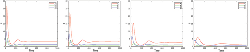As explained in Section 2, this parameter depends on the testing intensity which allows for early identification of infection of individuals. The parameter $\mathit{\alpha }$ can be used as an additional time-varying control variable, the effect of which is seen on Figure 2. The effect of testing is particularly high in suppressing the first pick of the disease. This can be explained by the immediate effect of testing when the effective reproduction number is close to the basic one, while later on the role of immunity of the recovered population dominates the effect of testing.

Figure 1. Endemic case in the long run (with $\mathit{\mu }=0$). Left to right $\mathit{S}$, $\mathit{I}$, $\mathit{R}$.

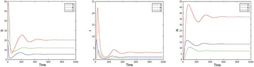
Figure 2. Evolution of $\mathit{I}$ (with $\mathit{\mu }=0$) for values of $\mathit{\alpha }=0.5,0.4,0.3,0.2$ (left to right).

We do not make such a comparative analysis for the other two control parameters, since we perform optimization with respect to them.

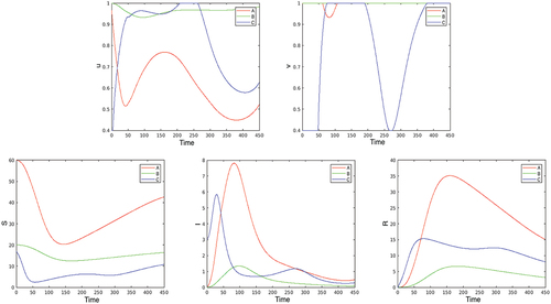
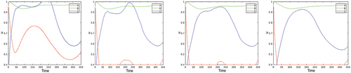
2. Next, we consider the optimal solutions of problem (2.5)–(2.7), (4.1)–(4.2) in the benchmark case. The first two plots on Figure 3 present the optimal controls; the corresponding $\mathit{S}$, $\mathit{I}$ and $\mathit{R}$ are given in the second three plots. Looking at the plot of $\mathit{u}$, it is remarkable that in the first days of the epidemic the optimal contact restriction at the ‘touristic’ location C (where the epidemic begins, as partly in Austria, for example) is extremely high, while the contact restrictions become persistently stronger in the big city A after about 20 days. The reason is that the disease quickly moves from the small city C to the large one, A, due to the intensive (touristic) visits from A to C. In contrast, the partial lock-down, $\mathit{v}$, is negligible at A, and that at C is (again) strong at the beginning and during the second wave of the disease after day 250.

Figure 3. Optimization with respect to both $\mathit{u}$ and $\mathit{v}$ in the benchmark case. The first two plots present the optimal controls $\mathit{u}$ and $\mathit{v}$, the second three plots give the corresponding $\mathit{S}$, $\mathit{I}$, and $\mathit{R}$.

Comparing the above results with those obtained when optimizing only with respect to $\mathit{u}$, we see that in the benchmark case the lock-down control $\mathit{v}$ plays a relatively minor role in the spread of the epidemic. Therefore, in the subsequent experiments, we use only $\mathit{u}$ as a control variable, fixing $\mathit{v}(\mathit{t})=1$.

3. The optimal control problem formulated in Section 4 is on a finite horizon. The question arises whether the optimal control substantially depends on the time horizon. This question is important for several reasons:

1. It is natural to consider the optimization problem (2.5)–(2.7), (4.2) on the infinite horizon $[0,\mathrm{\infty })$, therefore the issue of convergence of the solution of the problem on $[0,\mathit{T}]$ when $\mathit{T}\to \mathrm{\infty }$ is relevant (see the survey Aseev and Veliov (2019) about this issue, in general).

2. In practice, any policy has to be revised in the course of application in order to catch up with new information. In particular, the improved medical understanding of the disease, changes in the death rates, new variants of the pathogens, etc. may emerge. Then the optimization problem has to be resolved (in an infinite or long horizon), and the optimal control has to be applied on a short horizon only, before the next update. This is the essence of the so-called Model Predictive Control (MPC) method for assimilation of new measurements in stabilization or optimal control problems. We mention that MPC (see e.g. Raković and Levine (2019)) is the most widely applied method for process control in industry, but also for policy design in the context of epidemics, although its theoretical grounds seem not to be well adapted to the last context in the existing literature on mathematical epidemiology.

Figure 4 shows the optimal control $\mathit{u}$ for three time horizons. It is seen that the optimal controls are close to each other during the first about 50 days and are qualitatively similar in the first about 200 days. Thus, updating the control every month (or less) is a reasonable choice in the framework of Model Predictive Control (MPC).

Figure 4. Optimal control $\mathit{u}$ for time horizon $\mathit{T}=500,1000,2000$, cut at $\mathit{t}=450$.

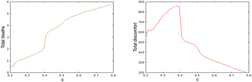
4. Comparative analysis: dependence on the activity rate of infected individuals $\mathit{\alpha }$, and on the contact rates $\mathit{c}$. First, we compare the optimal solutions for various values of the parameter $\mathit{\alpha }$. We remind that $\mathit{\alpha }$ can be decreased by increasing the testing effort. Only the size of the infected population is plotted in the first line of Figure 5, which shows that, as expected, the number of infected individuals is increasing as $\mathit{\alpha }$ increases, the total number of deaths (second line, right) is increasing correspondingly. The dependence of the total control ‘energy’ $\mathit{E}(\mathit{x},\mathit{\alpha }):={\int }_0^T(1-\mathit{u}(\mathit{t},\mathit{x}){)}^2\mathit{d}\mathit{t}$ (representing the social disutility), however, is more interesting. In the right plot on the second line of Figure 5 it is seen that the functions $\mathit{E}(x_1,\cdot )$ and $\mathit{E}(x_2,\cdot )$ (corresponding to locations $\mathit{A}$ and $\mathit{C}$) increase when $\mathit{\alpha }$ increases from $0.2$ to the threshold $\mathit{\alpha }\approx 0.37$, after that they decrease. This fact can be explained by the effect of herd immunity. The higher the value of $\mathit{\alpha }$ above the threshold, the more people obtain immunity from infection and the effect of contact restriction becomes relatively smaller. The reduction of the control ‘energy’ after the threshold, however, leads to a steep increase of the deaths. Remembering that $\mathit{\alpha }$ can be increased/decreased by decreasing/increasing the testing efforts, one can formulate the above finding in the following way: testing and contact restrictions (considered as policies) appear as substitutes below a certain threshold level for the testing effort, and as complements above this threshold.

Figure 5. Infected population in the optimal solution for values of $\mathit{\alpha }=0.2,0.3,0.4,0.5$ (first line), total number of deaths (second line left), and total “control energy” $\mathit{E}$ (second line right)—called “discomfort” on the plot—on $[0,\mathit{T}]$ as functions of $\mathit{\alpha }$.

Similar results are obtained when the multiplier $\hat{c}$ of the contact rates is varied, see Figure 6. For values of $\hat{c}$ above the threshold level $\hat{c}\approx 0.4$, the higher are the contact rates, the lower is the total of the applied control ‘energy’, although the total number of deaths increases faster. This means that for populations with intensive contacts between people the optimal contact restrictions are low; the optimizing decision-maker should rely more on the herd immunity. On the contrary, if the contact rates are small enough, then the decision-maker should make them even smaller by intensive contact restrictions.

Figure 6. Total number of deaths (left plot) and total social disutility (right plot) in the optimal solution for multiplier $\hat{c}$ of the contact rates varying between 0.2 and 0.8.

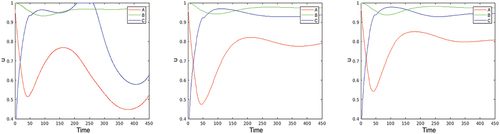
5. Finally, we investigate the dependence of the optimal contact restrictions $\mathit{u}$ on the discount rate $\mathit{r}$. It is remarkable that the control effort considerably increases with the discount rate, see Figure 7. The explanation of this fact is not obvious, because one can expect the opposite: higher $\mathit{r}$ means higher discount of the deaths in the future, hence less control action is required. However, higher $\mathit{r}$ also means that the future control and economic costs are more discounted, thus of lower value. The results on Figure 7 show that the second effect dominates. Indeed, a discount factor $\mathit{r}=0.00075$, for example, leads to approximately 56% decrease of value in 3 years, which is reasonable for the deaths, because one can expect a substantial progress of medication and medical service in three years, while the purely economic discount factor is normally about 10 times lower: $0.03/365\approx 0.00008$. This means that if a discounting is included in an economic-epidemiological model (as it is usual), then the economic and the epidemic parts should be differently discounted.

Figure 7. Optimal controls $\mathit{u}(\cdot ,\mathit{x})$ for values of discount $\mathit{r}=0,0.00075,0.0015,0.0030$.

6. Discussion

We develop a spatio-temporal epidemic model and focus on the investigation of human contact and mobility restrictions. The novel element of our work is the control theoretical approach to optimization of the policies. As a preliminary step, we obtain conditions for stability of the disease-free equilibria, and an explicit formula for the basic reproduction number.

The contact and mobility restrictions, the latter in the form of partial lock-down, are considered as control variables representing the policies. The optimal control problem aims at minimization of an inter-temporal combination of three components: the total number of deaths (or hospitalizations) due to the epidemic, the socio-economic cost of the policy measures, and the economic losses due to the epidemic and the partial lock-downs.

The particular scenarios studied in the paper involve three locations (e.g. cities) and the contact and mobility restrictions within and between them. We investigate the effects of the restrictions also in association with other measures such as the intensity of testing whether individuals are positive to the infection status.

Based on numerical experiments made with a 3-cities configuration (within the limitations of the benchmark model), we obtain several findings about the optimal policies that are summarized below.

1. We obtain an explicit formula for the basic reproduction number, which can be used in the usual way.

2. It is shown that in case of a disease with relatively long incubation period in part of which infected individuals are infectious, testing (leading to smaller labour participation of infected individuals (LPI)) is crucial, especially in suppressing the first wave of the epidemic. Later on, the immunity of the recovered population has a dominant role in comparison with the effect of testing.

3. There is a threshold of the LPI value below of which higher LPI leads to more restrictions at the optimum, and above which higher LPI leads to less restrictions accompanied, however, with a steep increase of deaths. The heard immunity is more efficient than restrictions in the latter case. Thus, testing and contact restrictions (considered as policies) appear as substitutes below a certain threshold level for the testing effort, and as complements above this threshold. This means that more testing efforts may lead to less/more optimal contact restrictions depending on whether the current testing is below/above a threshold value.

4. Similar threshold effect is observed for the dependence of the optimal contact restriction policy on the natural contact rates (that is, before the epidemics) of the population. For populations with intensive natural contacts between people the optimal contact restrictions are low; the optimizing decision-maker should rely more on the herd immunity. On the contrary, if the contact rates are small enough, then the decision-maker should make them even smaller by intensive contact restrictions. Of course, the number of deaths is smaller in the second case.

5. The numerical results also indicate that the optimal policy restricted to a relatively short initial interval does not substantially depend on the time horizon in which the optimization problem is solved. This allows for the application of the model predictive control method for policy updates based on current measurements.

Moreover, interesting properties of the timing and intensity of the contact restrictions in different locations are obtained, depending on the flows of people between the locations.

Overall, the paper provides useful insights into optimal control of outbreaks. Besides other spatial intervention scenarios, several extensions of the approach are possible: more detailed epidemic models including additional compartments such as exposed, asymptomatic infected, isolated, etc. Moreover, existing models involving vaccination, waning immunity, etc., can be embedded into spatial framework similarly as in the present paper. More interesting from a mathematical point of view is an extension with a distributed (not necessarily discrete) space. This leads to models in which the population compartments are represented by measures instead of finite-dimensional points. Optimal control problems in spaces of measures are currently under intensive investigation.

An extension would be the analysis of epidemic models to be accompanied by optimal control approaches in other societal areas. In particular at the socio-economic level, this is important since the implications of emerging health threats such as pandemics are not only in terms of public health but also critically affect other areas of society, the disruption of which may in turn have again consequences on public health.

Disclaimer

Te views expressed in this article are purely those of the authors and may not, under any circumstances, be regarded as an official position of the European Commission.

Acknowledgments

The authors are thankful to one of the reviewers of the paper for a remark about the non-symmetricity of $\mathit{A}$, and to Alberto Corella and Robert Israel for suggesting to us the proof of Lemma 3.1. This work was supported by the Austrian Science Fund (FWF) under grant No I-4571-N.

Disclosure statement

No potential conflict of interest was reported by the author(s).

Data availability statement

All data supporting the findings of this study are available within the paper.

Additional information

Funding

The work was supported by the Austrian Science Fund (FWF) [No I 4571-N].

Notes

1. More compartments can be involved in the model for more detailed description of the disease dynamics, similarly as in the single location models.

References

- Aguilar J, Bassolas A, Ghoshal G, Hazarie S, Kirckley A, Mazzoli M, Meloni S, Mimar S, Nicosia V, JJ R, et al. 2022. Impact of urban structure on infectious disease spreading. Sci Rep. 12(1):3816. doi: 10.1038/s41598-022-06720-8.
- Arino J, Van Den Driessche P. 2023. A multi-city epidemic model. Math Popul Studies. 10(3):175–193. doi: 10.1080/08898480306720.
- Aseev SM, Veliov VM. 2019. Another view of the maximum principle for infinite-horizon optimal control problems in economics. Russ Math Surv. 74(6):963–1011. doi: 10.1070/RM9915.
- Bertaglia G, Boscheri W, Dimarco G, Pareschi L. 2021. Spatial spread of COVID-19 outbreak in Italy using multiscale kinetic transport equations with uncertainty. Math Biosci Eng. 18(5):7028–7059. doi: 10.3934/mbe.2021350.
- Bloom DE, Kuhn M, Prettner K. 2020. Modern infectious diseases: macroeconomic impacts and policy responses. J Of Economic Literature. 60(1):85–131. doi: 10.1257/jel.20201642.
- Brauer F, Castillo-Chavez C, Feng Z. 2019. Mathematical models in epidemiology. Vol. 32, Berlin: Springer.
- Castillo-Chavez C, Bichara D, Morin BR. 2016. Perspectives on the role of mobility, behavior, and time scales in the spread of diseases. Proc Natl Acad Sci U S A. 113(51):14582–14588. doi: 10.1073/pnas.1604994113.
- Caulkins JPP, Grass D, Feichtinger G, Hartl RF, Kort PM, Prskawetz A, Seidl A, Wrzaczek S. 2021. The optimal lockdown intensity for COVID-19. J Math Econ. 93:102489. doi: 10.1016/j.jmateco.2021.102489.
- Chen D, Xue Y, Xiao Y, Ferrari M. 2021. Determining travel fluxes in epidemic areas. PLoS Comput Biol. 17(10):e1009473. doi: 10.1371/journal.pcbi.1009473.
- David JF, Iyaniwura SA. 2022. Effect of human mobility on the spatial spread of airborne diseases: An epidemic model with indirect transmission. Bull Math Biol. 84(63). doi: 10.1007/s11538-022-01020-8.
- David JF, Iyaniwura SA, Ward MJ, Fred B. 2020. A novel approach to modelling the spatial spread of airborne diseases: an epidemic model with indirect transmission. Math Biosci Eng. 17(4):3294–3328. doi: 10.3934/mbe.2020188.
- Diekmann O, Heesterbeek JAP. 2000. Mathematical epidemiology of infectious diseases. Wiley series of mathematical and computational biology. England: Wiley.
- Dontchev AL, Hager WW, Veliov VM. 2000. Second-order Runge-Kutta approximations in control constrained optimal control. SIAM J Num Anal. 38(1):202–226. doi: 10.1137/S0036142999351765.
- Geng X, Katul GG, Gerges F, Bou-Zeid E, Nassif H, Boufadel MC. 2020. A kernel-modulated SIR model for COVID-19 contagious spread from country to continent. PNAS. 118(21):e2023321118. doi: 10.1073/pnas.2023321118.
- Grimee M, Bekker-Nielsen Dunbar M, Hofmann F, Held L. 2021. Modelling the effect of a border closure between Switzerland and Italy on t e spatiotemporal spread of COVID-19 in Switzerland. Spatial Stat. 49:100552. doi: 10.1016/j.spasta.2021.100552.
- Hethcote HW. 1996. Modeling heterogeneous mixing in infectious disease dynamics. In models for infectious human diseases (eds. V. Isham and G. F. H. Medley). Cambridge, UK: Cambridge University Press; pp. 215–238.
- Jia Q, Li J, Lin H, Tian F, Zhu G. 2022. The spatiotemporal transmission dynamics of COVID-19 among multiple regions: A modeling study in Chinese provinces. Nonlinear Dyn. 107(1):1313–1327. doi: 10.1007/s11071-021-07001-1.
- Kaslow DC. 2021. Force of infection: a determinant of vaccine efficacy? NPJ Vaccines. NPJ Vaccines. 6(1):51. doi: 10.1038/s41541-021-00316-5.
- Kovacevic R, Stilianakis NI, Veliov VM. 2022. A distributed optimal control epidemiological model applied to COVID-19 pandemic. SIAM J Control Optim. 60(2):S221–S245. doi: 10.1137/20M1373840.
- Mazzoli M, Pepe E, Mateo D, Cattulo C, Gauvin L, Bajardi P, Tizzoni M, Hernando A, MEloni S, Ramasco JJ. 2021. Interplay between mobility, multi-seeding and lockdowns shapes COVID-19 local impact. PLoS Comput Biol. 17(10):e1009326. doi: 10.1371/journal.pcbi.1009326.
- Nakata Y, Roest G. 2015. Global analysis for spread of infectious diseases via transportation networks. J Math Biol. 70(6):1411–1456. doi: 10.1007/s00285-014-0801-z.
- Parino F, Zino L, Porfini M, Rizzo A. 2021. Modelling and predicting the effect of social distancing and travel restrictions on COIVD-19 spreading. J Royal Soc Interface. 18(175):20200875. doi: 10.1098/rsif.2020.0875.
- Raković SV, Levine WS. 2019. Handbook of model predictive control. BIrkhaeuser.
- Rapti Z, Cuevas-Maraver J, Kontou E, Liu DY, PG K, Barmann M, QY C, Kevrekidis GA. 2023. The role of mobility in dynamics of the COVID-19 epidemic in Andalusia. Bull Math Biol. 85(54). doi: 10.1007/s11538-023-01152-5.
- Schoot Uiterkamp MHH, Goesgens M, Heesterbeck H, van der Hofstad R, Litvak N. 2022. The role of inter-regional mobility in forecasting SARS-CoV-2 transmission. J R Soc Interface. 19(193):20220486. doi: 10.1098/rsif.2022.0486.
- Topirceanou A, Precup R-E. 2021. A novel geo-hierarchical population mobility model for spatial spreading of resurgent epidemics. Sci Rep. 11(1):14341. doi: 10.1038/s41598-021-93810-8.
- Van den Driessche P, Watmough J. 2008. Further notes on the basic reproduction number. In Brauer F, Van den Driessche P, and Wu J, editors. Mathematical epidemiology. Lecture notes in mathematics. Berlin Heidelberg: Springer; p. 159–178.
- Zakary O, Larrache, 2016. Effect of awareness programs and travel-blocking operations in the control of HIV/AIDS outbreaks: a multi-domains SIR model. Adv Differ Equ. 2016(1):169. doi:10.1186/s13662-016-0900-9.
- Zhang F, Jin Z. 2022. Effect of travel restrictions, contact tracing and vaccination on control of emerging infectious diseases: transmission of COVID-19 as a case study. Math Biosci Eng. 19(3):3177–3201. doi: 10.3934/mbe.2022147.