Clingo2DSR - A clingo-based software system for declarative spatial reasoning

ABSTRACT

We present a modified ground-and-solve approach based on the clingo Answer Set Programming (ASP) system to perform non-monotonic spatial reasoning tasks, Clingo2DSR. Our system is distinct from previous research integrating ASP with space in that it deals with complex real-world data and numerous time steps. Clingo2DSR is composed of (i) an input language defining spatial entities, functions, and relations; (ii) an external geometry database for performing spatial computations and checking spatial constraints; and (iii) a theory-based solving approach coupling symbolic ASP with external sources for sound and fast model search. We demonstrate our system on three real building models, in the context of architectural design, submitted for analyses and queries where spatial components play an important role.

KEYWORDS:

• Building Information Modelling
• Answer Set Programming
• spatial reasoning

1. Introduction

Declarative spatial reasoning (DSR) (Bhatt et al., 2011; Schultz & Bhatt, 2014) is a subfield of KR-driven AI research that is concerned with representing and reasoning about spatial knowledge using mixed quantitative and qualitative functions and relations, such as the distance or topological relationship between two polygons.

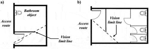
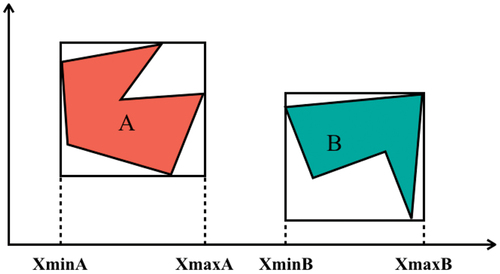
To illustrate this, we consider the application domain of building code compliance checking in the field of architectural design (Amor & Dimyadi, 2021; Dimyadi & Amor, 2013). The following building regulation is from the New Zealand Building Code (NZBC): There shall be no direct line of sight between an access route and a WC, urinal, bath, shower or bidet. Two acceptable layouts are shown in Figure 1. This building code elicits a qualitative spatial relation visible from between two quantitative spatial entities, access route and bathroom object.

Figure 1. Two acceptable layouts where the bathroom object is shielded from the vision limit line, adapted from (Department of Building and Housing, 2011).

A typical DSR task consists of checking such a building code on the digital representation of a building plan to deduce a violation. We can formalize a violation of this code as the following first-order logic rule:

where Entities denotes the set of all spatial entities in the building plan. The standard way of digitally representing buildings is referred to as Building Information Modelling (BIM). A particular BIM standard is a set of classes used to represent objects (e.g. walls, doors, windows, floors), and relationships (e.g. a building is composed of building storeys; a window fills a particular opening in a wall). A BIM model is an object-oriented instance of the BIM standard, where each BIM model object has a unique ID, a type, a geometry, and properties and relationships.

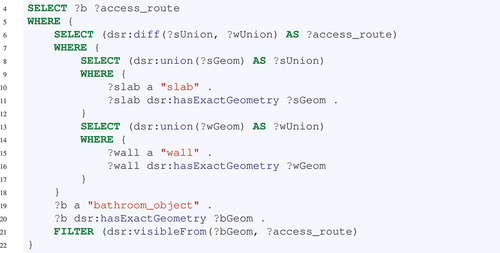
This example highlights two practical difficulties that arise when applying DSR to application domains such as building code compliance checking. The first challenge is concerned with knowledge engineering: “access route” has no formal definition in any of the widely used BIM standards such as Autodesk Revit or Industry Foundation Classes. Thus, the existence of “access route” objects in a given BIM model needs to be inferred based on context and domain knowledge. One interpretation of an “access route” is that its 2D footprint corresponds to walkable surfaces (e.g. slabs) subtracted by movement obstacles (e.g. walls). Using SPARQL-like syntax, this is translated into a stack of nested statements:

Similarly, the spatial relation “visible from” is ambiguous and open to interpretation. Important aspects that are not explicitly detailed in the building code include eye level of the viewer, their visual range, whether reflective surfaces, lighting and shadows are to be considered, and so on. This is a question of developing an appropriate domain-specific formalisation methodology that also uses spatial predicates.

From the perspective of a DSR tool provider (such as ourselves), such spatial predicates can not be hard-coded a priori based on predefined algorithms, as demonstrated by the example above, where different users will require different definitions of “visible from” and “access route.” In order for DSR to have effective industry impact and outreach, a user of DSR tools needs to be able to configure the underlying spatial libraries and geometry solvers.

The second challenge is that of runtime execution. A DSR rule such as our example that defines an “access route” needs to execute on large BIM models that may consist of thousands of building objects with large and detailed geometric representations, i.e. polygons consisting of thousands of vertices and edges. General search strategies are needed to prune the search space based on geometric data structures and heuristics. For example, two polygons cannot intersect if their bounding boxes do not intersect.¹ Thus, by pre-computing and organizing the bounding boxes of each polygon into an appropriate data structure, a search strategy can be devised that avoids computing the differences of polygons whose bounding boxes do not intersect, significantly speeding up the execution of such a rule on many BIM models.

However, such heuristics should not be introduced into the rule by the user, but rather should be “built-in” to the DSR solver. Such a DSR solver should be able to take the example code snippets above that formalize the building code violation and the definition of an “access route” and automatically apply appropriate runtime heuristics, so that the user-defined rules remain clean, simple and clear for the user, but execute rapidly when applied to large BIM models.

In this paper, we present one approach for tackling these issues by leveraging the strengths of declarative problem solving. The approach we present uses the logic programming language Answer Set Programming (ASP) to push runtime concerns down to the solver so that the user-defined knowledge base stays clean and manageable.

1.1. Problem statement and research questions

Having opted to explore ASP as a vehicle for addressing the aforementioned challenges, our more focused problem statement in this paper is how to enable ASP to operate on spatial predicates. We propose to use the theory solving capabilities of ASP to calculate spatial expressions based on chosen spatial calculi and theories. In pursuing this approach, we have found that DSR poses three new challenges to theory-enhanced ASP.

Firstly, it is impractical to encode large, complex geometric data as plain ASP facts. That is, continuing with the example application domain of building code compliance checking, BIM model geometry data could be represented as the following ASP fact where the footprint of an object is a polygon bounded by a list of 2D line segments (represented as a list of 2D vertices), constructed recursively with the predicate $\mathit{cons}/2$.

However, when scaling up to real-world BIM models, the size of the text file containing these facts grows orders of magnitude larger than the original BIM model data file. The large number, and large size of these facts drastically limits the size of BIM models that can be handled in practice.

Research Question RQ1.

How can ASP programs represent, search over, and manage large, complex geometry data in an efficient and scalable way?

Secondly, the common way that ASP solvers deal with numerical data, such as integers and (simple) arithmetic expressions, does not scale up to geometry computations in general.

In a step in ASP referred to as grounding in the presence of variables, all possible combinations of feasible variable values are generated (and then later used in the subsequent “solve” step). This works well when variables range over a small set of integers, but does not work well when variable values are the result of more complicated geometric computations.

This is even more of an issue when almost all possible combinations of such variable values are trivially not of interest to the user. For example, when trying to calculate the difference of slabs and walls in our previous “access route” definition, almost all slabs and walls are already disjoint, and thus ASP grounding will generate a tremendous number of trivially redundant variable values. In more technical terms, a large number of ASP rules can lead to a blowup of the ground instantiation, of which only a tiny fragment is spatially consistent (Gebser et al., 2018). We refer to this issue as the grounding bottleneck for spatial predicates.

Research Question RQ2.

How can the grounding step in ASP be adapted to incorporate spatial consistency checks to overcome the grounding bottleneck for spatial predicates?

Finally, in many application domains, spatial data undergo a series of numerical computations that are state-dependent, which contradicts the declarative character of symbolic ASP. For instance, one may define an ASP rule that calculates the intersection of two polygons, and then “enlarges” (dilates) this intersection. The dilation calculation cannot be performed before the intersection calculation, and thus there is a dependency between these two parts of the rule. The issue here is that ASP rules (and also clauses within a rule) should not be treated as having a particular execution order as this breaks the declarative character of ASP.

Research Question RQ3.

How can dependencies between spatial predicates in a rule, and between rules, be handled in ASP without breaking the declarative character of ASP?

1.2. Contributions

To address research questions RQ1-RQ3, we present a modified ground-and-solve approach based on the clingo Answer Set Programming (ASP) system, Clingo2DSR. We have developed the system in the context of 4D BIM models with large, complex geometric data and numerous time steps. Our key contributions in this paper are:

Contribution C1. We specify an input language defining entities, functions, and relations in common spatial domains and their corresponding theory extensions in Clingo2DSR (Section 5); this addresses RQ1.

Contribution C2. We develop an approach for integrating an internal geometry database to create, maintain, and update geometric representations of spatial entities in sync with ASP model search, i.e. for grounding symbolic atoms with numerical data and computing spatial functions and relations (Section 6); this addresses RQ1, RQ2.

Contribution C3. We develop a new spatial checker to efficiently prune the search space by checking spatial constraints on partial model assignments, and a dedicated spatial propagator to organize symbolic ASP rules into a cascade of spatial evaluations which reflects their implicit dependencies (Sections 6.2 and 7); this addresses RQ2, RQ3.

Moreover, we present two empirical experiments that assess the performance and scalability of Clingo2DSR, and we present three case studies in the application domain of building code compliance checking that serve to demonstrate that Clingo2DSR can be used for diverse tasks, and that it can run on large-scale building models with practical runtimes (Section 8). We have made the source code for Clingo2DSR along with test cases freely available for download.²

1.3. Contributions beyond our previous spatial reasoning systems

The immediate predecessor system to Clingo2DSR is a system we developed called ASP4BIM, a term first coined in (Hjelseth & Li, 2021). ASP4BIM is a declarative spatial reasoner in the context of checking geometric and topological constraints in BIM models. However, in our previous research and development of ASP4BIM ((Li, Fitzgerald, et al., 2022; Li, Schultz, et al., 2022)) we focus exclusively on the syntax of representing layered, multifaceted spatial problems using ASP, while in the present paper, we explain, for the first time, the implementation details of the underlying solver engine, Clingo2DSR.

Clingo2DSR is a mixed quantitative and qualitative spatial reasoner that builds spatial theory extensions into Answer Set Programming. This is done by representing spatial functions and relations over spatial entities as theory atoms which are evaluated at various solving steps during theory propagation. This is an important theoretical contribution beyond our previous work on ASP4BIM and other systems (e.g (Bhatt et al., 2011; Walega et al., 2017).

ASP4BIM has previously been evaluated on a variety of real-world applications ranging from automated building code checking (Li, Dimyadi, et al., 2020), construction safety analysis (Li, Schultz, et al., 2020), to renovation design decision-support (Kamari et al., 2019). In this paper we go beyond our earlier prototype implementations by showing faster runtimes through an empirical evaluation in Section 8.1 (contribution C2), and having a more mature, developed, underlying framework based on theory atoms and the spatial cascading technique (contributions C1 and C3).

The four following system details mark a clear departure and improvement of Clingo2DSR over ASP4BIM, detailed in Sections 6.1–6.4, respectively:

• In Clingo2DSR, spatial entities are represented by object identifiers that are uniquely and deterministically mapped to geometry identifiers in an internal geometry database. Previously, in ASP4BIM, we encoded geometry identifiers as symbolic ASP facts which leads to grounding bottlenecks, as geometry identifier variables can be bound to inconsistent object identifiers during grounding (detailed in Section 6.1).

• Cascading spatial calculations are performed in the correct order that is automatically inferred from theory atoms with non-strict and defined semantics. Previously, in ASP4BIM, we encoded spatial functions as aggregates, which also leads to grounding bottlenecks as the aggregates can be grounded with inconsistent geometry identifiers (detailed in Section 6.2).

• In Clingo2DSR, spatial data structures are deduced on the fly and used for constraint-driven theory solving to shortcut unnecessary numerical evaluations, which was not a feature supported in ASP4BIM. Spatial data structures are stored as dictionaries $\_\mathit{exts}$ and $\_\mathit{aabbs}$ in the geometry database which are used in symbolic ASP to infer size and topology relations by numerical comparisons that are computationally inexpensive (detailed in Section 6.3).

• In Clingo2DSR, an SMT solver is used to check spatial consistency of partial assignments in hypothetical reasoning (where competing assumptions can be derived), which was not a feature supported in ASP4BIM. If partial assignments are inconsistent, spatial nogoods are recorded and theory propagation backtracks. If partial assignments are consistent (spatial constraints are jointly satisfiable and have a witness), the assumptions are added to the dictionary $\_\mathit{rels}$ in the geometry database to continue theory propagation (detailed in Section 6.4).

2. Related work

Numerous researchers have addressed the compatibility of ASP semantics with external sources, rules, and ontologies, e.g. deductive databases (Calimeri et al., 2017), Semantic Web (Eiter et al., 2008), Web Ontology Languages (Leone et al., 2019), etc. While reasoning about BIM models falls within the general category of integrating ASP with external data and evaluations, also called value invention (Calimeri et al., 2007), in addition it emphasizes an implicit set of domain-specific knowledge and constraints, and a two-way information exchange between symbolic ASP and BIM semantics and geometry (Eiter et al., 2017).

Declarative spatial reasoning systems have been developed that support spatial reasoning within logic programming, such as CLP(QS) (Bhatt et al., 2011; Schultz & Bhatt, 2014, 2015) and ASPMT(QS) (Walega et al., 2015, 2017). The key point of departure in Clingo2DSR is being able to handle industry-scale BIM models which we achieve by integrating ASP with a geometry database combined with the cascading technique that we present in Section 6.2, i.e. both CLP (QS) and ASPMT (QS) have no mechanisms for representing and reasoning over numerous, large geometries beyond plain logic programming facts (research question RQ1).

Other research efforts have specifically focused on Building Information Modelling via logic programming, toward a unified approach that seamlessly combines the ontological (non-geometric) and geometric aspects of digital building representations. For example, InSpace3D (Schultz & Bhatt, 2013; Schultz et al., 2017) is a middleware framework based on CLP(QS) that specializes in predicting human-centered behavior and experience by generating so-called spatial artefacts. Owing to its foundations in Prolog (via CLP(QS)) the differences between InSpace3D and Clingo2DSR encompass all standard differences between Prolog and ASP, and InSpace3D primarily focuses on generating and analyzing the computation of spatial artifacts whereas Clingo2DSR is more broadly focused on enabling ASP-based reasoning on (for example) industry-scale BIM models.

As another example of research that utilizes logic programming for BIM, Arias et al. (Arias et al., 2022) present a framework that integrates CLP and ASP, tailored for representing and reasoning about BIM models. Their Constrained ASP system s (CASP) (Arias et al., 2018) can reason with a rule set that has non-stratified negation, and, interestingly, supports constructive negation.³ One key difference with Clingo2DSR is that their approach, fascinatingly, avoids the grounding step that is usually undertaken in ASP, whereas Clingo2DSR seeks to improve the grounding step to permit spatial reasoning on knowledge bases with a large number of semantic facts, spatial rules, and large, complicated geometries, as is common in application domains such as building code compliance checking.

3. Background

3.1. Answer set programming syntax and semantics

3.1.1. ASP syntax

In ASP-Core-2 syntax (Calimeri et al., 2019a), a term is a constant, variable, arithmetic term, or function term. An atom is an expression of the form $\mathit{p}(t_1,\dots ,t_n)$ where $\mathit{p}$ is a predicate symbol and each $t_i$ is a term (for $1\le \mathit{i}\le \mathit{n}$). A classical atom is either an atom $\mathit{p}$, or a negated atom $\mathrm{\neg p}$. A negation as failure (naf) literal is a classical atom $\mathit{a}$ or $\mathbf{not}\mathit{a}$. We refer to the complement of a classical atom $\mathit{a}$, denoted $-\mathit{a}$: if $\mathit{a}$ is an atom $\mathit{p}$, then $-\mathit{a}=\mathrm{\neg p}$, and if $\mathit{a}$ is a negated atom $\mathrm{\neg p}$ then $-\mathit{a}=\mathit{p}$.

A rule is an expression of the form

$\mathit{h}:-b_1,\dots ,b_m.$

where $\mathit{h}$ is a classical atom, and $b_1,\dots ,b_m$ are literals, for $0\le \mathit{m}$. The classical atom $\mathit{h}$ is called the rule head, and the conjunction $b_1,\dots ,b_m$ is called the rule body. A rule with $\mathit{m}=0$ is called a fact, and a rule with the head omitted is called a constraint. A program is a finite set of rules.

Strings beginning with uppercase letters denote variables, strings beginning with lowercase letters denote constants (i.e. predicates with zero arguments). A term with no variables is said to be ground (similarly defined for atoms, classical atoms, literals, rules, and programs).

A choice element is an expression of the form $\mathit{a}:l_1,\dots ,l_n$ where $\mathit{a}$ is a classical atom and $l_1,\dots ,l_n$ are literals. A choice rule is an expression of the form

$\{e_1;\dots ;e_n\}:-b_1,\dots ,b_m.$

where $e_1;\dots ;e_n$ are choice elements, and $b_1,\dots ,b_m$ are literals.

4. ASP Semantics.

The Herbrand universe of a program $\mathit{P}$ is a set consisting of all integers and ground terms that can be constructed from constants and predicate symbols appearing in $\mathit{P}$. A Herbrand interpretation of program $\mathit{P}$ is a subset of the set of all ground classical atoms constructed from predicate symbols appearing in $\mathit{P}$, and with all arguments being elements of the Herbrand universe (i.e. a Herbrand interpretation of $\mathit{P}$ is a subset of the Herbrand base of $\mathit{P}$).

A ground instance of a rule $\mathit{r}$ is the result of applying a substitution to $\mathit{r}$ that maps every variable in $\mathit{r}$ to an element of the Herbrand universe. The ground instantiation of a program $\mathit{P}$ is the set of all ground instances of rules in $\mathit{P}$.

A literal of the form $\mathit{a}$ (where $\mathit{a}$ is a classical atom) is true with respect to interpretation $\mathit{I}$ if $\mathit{a}\in \mathit{I}$. A literal of the form $\mathbf{not}\mathit{a}$ is true with respect to interpretation $\mathit{I}$ if $\mathit{a}\in \mathit{I}$, and false if $\mathit{a}\in \mathit{I}$. An interpretation is inconsistent if there exists an atom $\mathit{p}$ such that $\{\mathit{p},\mathrm{\neg p}\}\subseteq \mathit{I}$, and consistent otherwise.

A (ground) rule of the form $\mathit{h}:-b_1,\dots ,b_m$, in the ground instantiation of program $\mathit{P}$, is satisfied with respect to interpretation $\mathit{I}$ if $\mathit{h},b_1,\dots ,b_m$ are all true, or if at least one of $b_1,\dots ,b_m$ is not true. Constraints (i.e. rules missing a head) are only satisfied when at least one of $b_1,\dots ,b_m$ is not true.

An interpretation is a model of $\mathit{P}$ if every rule in the ground instantiation of $\mathit{P}$ is satisfied. The reduct of $\mathit{P}$ with respect to interpretation $\mathit{I}$ is the set of rules in the ground instantiation of $\mathit{P}$ where every literal in the body is true with respect to $\mathit{I}$. An interpretation $\mathit{I}$ is an answer set of $\mathit{P}$ if it is a model of $\mathit{P}$, and there is no proper subset of $\mathit{I}$ that is a model of the reduct of $\mathit{P}$.

Default reasoning plays an important role in building code compliance checking, especially with respect to knowledge representation, where deontic operators are often used in (natural language) building codes (Dimyadi et al., 2017).

Informally, a default rule (Reiter, 1980) consists of prerequisite formulae, justification formulae, and a conclusion formula with the meaning that: if the prerequisites are true, and the justifications are not known to be false (i.e. consistent with a given interpretation) then one can tentatively infer the conclusion.

We encode default rules as ASP rules as follows. Let $\mathit{c}$ be a classical atom corresponding to the default rule conclusion, let $p_1,\dots ,p_n$ be classical atoms corresponding to default rule prerequisites, and let $j_1,\dots ,j_m$ be classical atoms corresponding to default rule justifications, then the corresponding ASP default rule is:

$\mathit{c}:-p_1,\dots ,p_n,\mathbf{not}-j_1,\dots ,\mathbf{not}-j_m.$

We use the term default reasoning to mean that we explicitly express domain knowledge in form of default rules encoded as ASP programs. The use of default rules improves the quality of a compliance checking rule base by making it more manageable (maintainable, readable, extensible) rather than explicitly enumerating all possible scenarios in the form of purely deductive rules. Furthermore, we use default reasoning to handle tasks where the conclusions are drawn tentatively in the absence of key details in BIM models that would contradict the conclusion. For example, a BIM model space object can be missing details that are necessary to determine if it serves as an access route. In such cases, we can use default reasoning to assume that space $\mathit{s}$ is an access route if we can not prove that it is not an access route.

Hypothetical reasoning is used when the BIM model lacks certain key pieces of information. That is, if the design is incomplete we may be able to make plausible hypotheses that fill in the missing details that serve to explain the details that are given in the design. In this context, the BIM model is treated as the “observations,” i.e. those details that the BIM model designer has asserted and thus which we take as facts of the design. On the other hand, a design may be incomplete in the following sense. Consider, for example, that in order to install a doorway, one must commit to various details about the door panel, e.g. there is either a door panel or not, and if there is a panel then it can be a sliding panel, left hinged, right hinged, swinging inwards, swinging outwards, and so on. However, at the design stage, such details about the door panel may be absent.

Suppose that the designer has asserted that a particular space object $\mathit{s}$ is an access route, which we take as an “observation” of the design. Note that, by definition, there must be at least one doorway connecting to the access route through which occupants can enter and exit the route, and so the existence of a suitable connecting doorway is necessary to explain the existence of the access route. To ensure safe egress in emergencies, NZBC (and other building codes) require that doors should not swing into access routes, and thus, in NZBC compliant buildings, spaces that doors swing into cannot be access routes (the rule).

We can thus consider hypotheses about under-specified door panels of doors that connect to the access route that serve to explain the existence of the access route. We express this in ASP with a choice rule with both upper and lower cardinality constraints set to 1. The implication of the door swinging inwards is that the adjacent space $\mathit{s}$ is not an access route, due to obstructed clearance. If the observation is that $\mathit{s}$ is an access route, then we can counterfactually hypothesize that door $\mathit{d}$ swings outwards.⁴

3.2. Theory solving in ASP

Classical ASP is primarily a symbolic programming language that only supports built-in data types, e.g. integers and strings, and basic arithmetic operations e.g. addition and multiplication (Calimeri et al., 2019b). This severely limits the use of ASP with numerical data and computations, which is a ubiquitous feature of real-world applications.

To overcome this limitation, Answer Set Programming Modulo Theories (ASPMT) gives theory-specific meanings to ASP predicates so that an ASP program can be interpreted and solved with respect to background theories such as real numbers, linear arithmetic, and difference logic.

In the prominent ASP system clingo, theory extensions are implemented in two steps. First the grounder gringo is extended with theory definitions so that theory atoms are represented using ASP’s built-in modeling language. Then the solver clasp is enhanced with a theory propagator to i) propagate modulo theories, and ii) record nogood constraints with respect to theories when a model assignment has conflicts.

From a theoretical perspective, Bartholomew and Lee (Bartholomew & Lee, 2014) proposed a general framework, called ASPMT2SMT, to translate a small fragment of ASPMT instances into Satisfiability Modulo Theories (SMT) instances, then use SMT solvers to compute stable models. From an implementation perspective, numerous software prototypes extend clingo with background theories: clingoDL (Gebser et al., 2016) based on difference logic, clingoLP (Janhunen et al., 2017) based on linear constraints, clingcon (Mutsunori et al., 2017; Ostrowski & Schaub, 2012) based on constraint programming, eclingo (Cabalar et al., 2020) based on epistemic logic, and telingo (Cabalar et al., 2018, 2019) based on temporal equilibrium logic for finite traces.

4. Spatial theory extensions

In the prominent ASP system clingo, theory atom definitions are declared in two ways:

where $\mathit{p}$ is a predicate name and $\mathit{k}$ its arity, each ${\mathrm{♢}}_i$ is a theory operator, $\mathit{t}$ and $\mathit{t}{ }^{\mathrm{\prime }}$ are theory term definitions, and $\mathit{o}$ indicates where in a rule (i.e. head, body, or both) the theory atom is allowed to occur (Gebser et al., 2016; Kaminski et al., 2021).

A theory atom is of the form $\{C_1:L_1;\dots ;C_n:L_n\}\mathrm{♢}\mathit{c}$, where each $C_i$ is a tuple of theory terms according to definitions of $\mathit{t}$, each $L_i$ is a tuple of conditions, $\mathit{a}$ is an atom over predicate $\mathit{p}/\mathit{k}$, $\mathrm{♢}$ is a declared theory operator, and $\mathit{c}$ is a theory term according to definitions of $\mathit{t}{ }^{\mathrm{\prime }}$. Theory atoms are interpreted based on the invoked background theories (difference logic, linear constraints, etc.). That is, a theory atom denotes a theory constraint and is solved by predefined decision procedures, e.g. a conjunction of difference constraints is satisfiable if and only if the corresponding inequality graph has no negative cycles.

We employ the above syntax to define theory term spatial_term and theory atoms such as &union/1 and &topology/1 in Lines $32$-$34$. A description of these theory atoms and their associated spatial functions and relations are provided in Section 5.

Theory atoms natively support on-demand grounding, so that spatial evaluations that are computationally costly can be delayed until their corresponding literals are assigned True during propagation. This means that, spatial computations are only performed when their associated theory atoms are derived from the logic program, and spatial constraints are only enforced when their associated theory atoms are True.

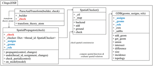
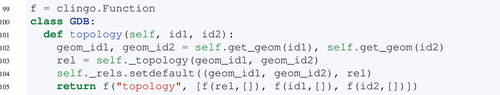
System architecture In Clingo2DSR, spatial theory solving is implemented via Clingo’s built-in Python API (see Figure 2). First, the ParseAndTransform (PAT) parses a logic program into a guess part and a check part ($\_\mathit{check}$). Then, the PAT transforms theory atoms and builds a new logic program ready for the SpatialPropagator (SP). The SP grounds the guess part, propagates assignment based on spatial theories, and checks partial assignment against the check part in the SpatialChecker (SC). Spatial evaluations associated with theory atoms are performed in the Geometry Database (GDB), and the results of these evaluations are sent back to the SP by shared attributes such as $\_\mathit{assigns}$ and $\_\mathit{rels}$ to advance propagation.

Figure 2. Class diagram of spatial theory solving via Clingo’s python API.

Furthermore, the SC is natively integrated with theory nogoods of the form $\{p_1,\dots ,p_m,\mathrm{\neg }{p}_{\mathit{m}+1},\dots ,\mathrm{\neg }{p}_n\}$ that prohibit $p_1,\dots ,p_m$ to be True and $\mathrm{\neg }{p}_{\mathit{m}+1},\dots ,\mathrm{\neg }{p}_n$ to be False simultaneously. In terms of spatial theories, nogoods reflect tautologies and contradictions such as two polygons cannot be disjoint and overlap, or a proper part of a polygon must be smaller than the polygon. This is encoded as the following constraints under the program directive $\mathit{check}$, so the SP checks partial assignments against them for spatial consistency.

A nogood constraint is unit when exactly one of its literals $\mathit{\delta }$ is not in the assignment. This triggers unit propagation where we add $\mathrm{\neg \delta }$ to the assignment as we know that $\mathit{\delta }$ cannot be included in the assignment (otherwise the nogood is violated) (Gebser & Schaub, 2006).

In Clingo2DSR, if both $\mathrm{overlaps}(\mathrm{a},\mathrm{b})$ and $\mathrm{disjoint}(\mathrm{a},\mathrm{b})$ are in the assignment, the SP uses backjumping to undo the last assignment so the conflict is resolved. Similarly, if $\mathrm{proper}\_\mathrm{part}(\mathrm{a},\mathrm{b})$ is in the assignment, the SP propagates adds $\mathrm{size}(\mathrm{smaller},\mathrm{a},\mathrm{b})$ to the assignment by unit propagation.

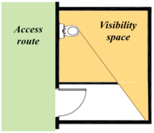
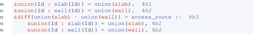
Revisiting the NZBC code In (Figure 3b), we illustrate an alternative interpretation of the privacy code as “the visibility space of a bathroom object should not overlap with an access route.”

Figure 3. An alternative interpretation of the privacy code based on visibility space, regions from which an object is visible (Bhatt et al., 2012).

This DSR task is executed in several steps. Firstly, the visibility space of a bathroom object is computed using the spatial theory atom $\mathit{isovist}$. In the following, when the variable $\mathit{B}$ is bound to a bathroom object, the rule fires and the spatial function associated with $\mathit{isovist}$ is computed in the GDB.

Secondly, an access route is computed as the difference between the union of all slabs and the union of all walls. This is expressed using spatial theory atoms with $\mathit{union}$ and $\mathit{diff}$:

In Clingo2DSR, the PAT adds a location argument (i.e. “body” or “head”) to spatial theory atoms. In this way, theory atoms in Line $50$ and $53$ (resp. Line $51$ and $54$) become distinct from the solver’s perspective. As a result, they are assigned different solver literals $h_1$ and $b_1$ (resp. $h_2$ and $b_2$) by the SP. In doing so, the SP also creates an internal dictionary to match transformed theory atoms that only differ by their location argument.

In addition, the SP adds the following clauses to force matching theory atoms with literals head and body, to always have the same truth value.

This means, whenever the literal $h_1$ (resp. $h_2$) is assigned True, the literal $b_1$ (resp. $b_2$) is also assigned True. In this way, we force theory atoms to have defined and non-strict semantics (Kaminski et al., 2021), that is, spatial theory atoms must be derived through the logic program, and spatial evaluations are only performed when the associated theory atoms are True.

During initialization, the head literals $h_1$ and $h_2$ become True as they are facts. At the same time, the body literals $b_1$ and $b_2$ become True, due to the above clauses. This causes the rule in Lines $52$-$54$ to fire, so that the head literal $h_3$ in Line $52$ also becomes True.

During propagation, the SP sends the head literals from the current assignment, i.e. $h_1$, $h_2$, and $h_3$, to the GDB for spatial evaluations. The GDB analyses the associated theory atoms, and deduces an implicit execution order by recursively computing spatial functions whose arguments are present in the internal geometry database. Specifically, the unions associated with $h_1$ and $h_2$ are first computed, as the slabs and walls are native BIM objects. Then, the difference associated with $h_3$ is computed, after the unions are added to the internal geometry database.

In this way, spatial theory atoms are organized into a cascading series as shown in Figure 4, so their associated calculations are only performed in the solving steps where they are included in the assignment. This avoids grounding bottlenecks as computationally expensive numerical evaluations are delayed until they are needed to propagate the assignment.⁵

Figure 4. Cascading spatial evaluations.

Finally, we use the spatial theory atom with &topology to deduce the topological relation between a visibility space and an access route.

This sends a pair of visibility space and access route objects to the GDB, where their topological relation $\mathit{R}$ is derived, which adds a new predicate $\mathit{topology}(\mathit{R},\mathrm{\_},\mathrm{\_})$ to the program. If $\mathit{R}$ is overlap, the following rule fires, so we conclude that the privacy clause is violated.

We note that a very elegant and more declarative re-formulation of the rule, that our current GDB implementation does not support, is a follows⁶

To handle such rules, the GDB system would need to recognize and “freeze” constraints, so that the topology evaluation is only performed once the visibility space and access route have been computed. In our current implementation we ask the programmer to specify the order explicitly, and rely on the default ASP ground-and-solve procedure to deduce the corresponding execution order, and thus we highlight this improvement of the GDB as future work.

5. Input language

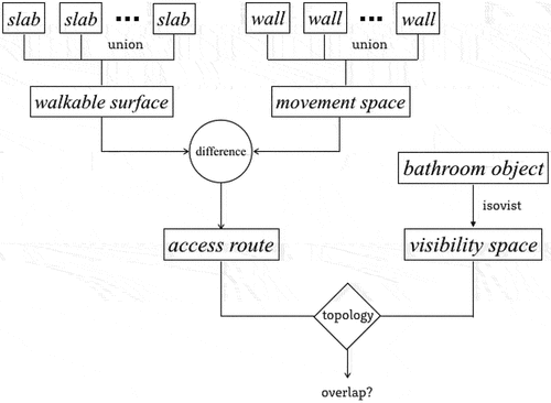
In the following, we present the input language of Clingo2DSR based on theory atoms. In particular, we use the Geometry Database (GDB) to ground spatial domains with numerical data, and evaluate spatial functions and relations with external libraries and solvers. In Clingo2DSR, GDB is implemented as a Class object. Figure 5 shows GDB’s built-in attributes and methods. In Section 6, we detail various optimizations techniques implemented in the GDB. In Section 7, we detail the interplay between GDB and the modified ground-and-solve approach in Clingo2DSR via theory propagation.

Figure 5. Class attributes and methods for the geometry database.

5.1. Spatial domains

Spatial domains in Clingo2DSR are defined as follows. A 2D point is a pair of reals $(\mathit{x},\mathit{y})$. A 3D point is a triple of reals $(\mathit{x},\mathit{y},\mathit{z})$. A line segment is a pair of 2D or 3D points $(p_1,p_2)$. A circle or sphere is a 2D or 3D point with a positive real (i.e. radius) $(\mathit{p},\mathit{r})$. An (axis-aligned) rectangle is a pair of points $(p_{\mathit{min}},p_{\mathit{max}})$ constructed from its minimum and maximum coordinates.

A polygon or polyhedron is a set of boundaries and a set of holes such that no two boundaries intersect and every hole is a non-tangential part of a boundary (i.e. contained within the boundary without touching the boundary edges or surfaces). Each contour (boundary or hole) of a polygon is a list of 2D points (vertices) $\mathit{V}=p_1,\dots ,p_n$. Each contour (boundary or hole) of a polyhedron is a list of 3D points (vertices) $\mathit{V}=p_1,\dots ,p_n$ and a set of triangular faces $f_1,\dots ,f_m$ where each face is a triple of vertices $v_i,v_j,v_k\in \mathit{V}$.

A spatial object $\mathit{o}\in \mathit{D}$ is a variable associated with a spatial domain $\mathit{D}$ (e.g. the domain of $2\mathit{D}$ points). Spatial objects can have quantitative (numeric) configurations with ground constants, or qualitative (symbolic) representations with free variables, or a combination of the two.

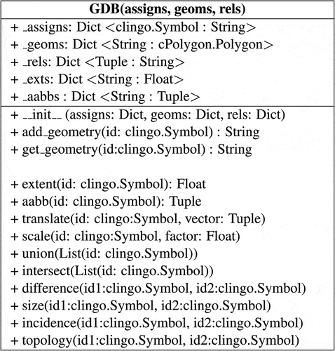
Clingo2DSR encodings As a prerequisite, we construct an external geometry database, _repr, to map IDs of BIM objects to their surface mesh representations in string format. In the following, the BIM object identified by “id1” is mapped to a list of oriented boundary vertices (2D points) in _repr.

If this BIM object becomes ground in theory atoms, the function add_geom uses “id1” to retrieve its geometric representation from _repr, constructs a shape (e.g. polygon), and returns a fresh geometry ID, geom_id.

During this step, “id1” is mapped to geom_id via dictionary _assigns, then geom_id is mapped to the shape via dictionary _geoms. For BIM objects, their geometry IDs are integers that are the length of _geoms at the time of the creation, incremented by 1.

In this way, we ensure that only the necessary spatial objects are constructed, as their associated theory atoms must be derived from the logic program. Moreover, the geometry IDs of spatial objects can be retrieved in later solving steps using the function get_geom, when they are needed for subsequent spatial functions or relations.

In the GDB class, the functions add_geoms and get_geom are implemented using clingo’s Python API as follows:

5.2. Spatial relations

Given a set of spatial objects $\mathit{O}$, a spatial relation $\mathit{r}$ of arity $\mathit{n}$ is asserted as a constraint that must hold between objects $o_1,\dots ,o_n\in \mathit{O}$, denoted $\mathit{r}(o_1,\dots ,o_n)$. For example, if $\mathit{dr}$ is the topological relation discrete,⁷ and $\mathit{O}$ is a set of polygons, then $\mathit{dr}(o_4,o_9)$ denotes the constraint that polygons $o_4,o_9\in \mathit{O}$ must be discrete.

Other notable spatial calculi such as $\mathcal{O}\mathcal{P}\mathcal{R}\mathcal{A}$ (Moratz, 2006), DE-9IM (Egenhofer & Franzosa, 1991), and $\mathcal{L}\mathcal{R}$ (Scivos & Nebel, 2005) propose sets of qualitative spatial relations to describe the topology, orientation, and incidence between two spatial objects (see Figure 6). In Table 1, we define a non-exhaustive list of size, incidence, and topology relations.

Figure 6. Topological relation partial overlap between two regions as defined in $\mathcal{R}\mathcal{C}\mathcal{C}$ −5, and incidence relation inside between points and regions.

Table 1. Spatial functions in Clingo2DSR

Spatial Functions	Description	ASP theory atoms
$\mathrm{extent}:$ $\mathrm{Region}\to \mathbb{R}$	Area for 2D regions or volume for 3D regions.	&extent{Region} = real
$\mathrm{centre}:$ $\mathrm{Region}\to \mathrm{Point}$	Centre point of region.	&centre{Region} = point
$\mathrm{aabb}:$ $\mathrm{Region}\to \mathrm{Box}$	Minimum axis-aligned bounding box of region.	&aabb{Region} = box
$\mathrm{distance}:$ $\mathrm{Region}\times \mathrm{Region}\to \mathbb{R}$	Minimum distance between two regions.	&distance{Region, Region} = real
$\mathrm{shift}:$ $\mathrm{Region}\times \mathrm{Point}\to \mathrm{Region}$	Translates region by the given vector point.	&shift{Region + Point} = region
$\mathrm{scale}:$ $\mathrm{Region}\times \mathrm{Point}\to \mathrm{Region}$	Scales region by the given vector point w.r.t its centre.	&scale{Region * Point} = region
$\mathrm{rotate}:$ $\mathrm{Region}\times \mathbb{R}\to \mathrm{Region}$	Rotates region by the given angle w.r.t. its centre.	&rotate{Region, Angle} = region
$\mathrm{flip}:$ $\mathrm{Region}\times \mathrm{Segment}\to \mathrm{Region}$	Flips region w.r.t the given line segment	&flip{Region\Segment} = region
$\mathrm{offset}:$ $\mathrm{Region}\times \mathbb{R}\to \mathrm{Region}$	Inflates or deflates region by the given distance	&offset{Region, Distance} = region
$\mathrm{union}:$ $\mathrm{Regio}{\mathrm{n}}^{\mathrm{N}}\to \mathrm{Region}$	Union of a set of regions.	&union{Region;} = region
$\mathrm{intersect}:$ $\mathrm{Regio}{\mathrm{n}}^{\mathrm{N}}\to \mathrm{Region}$	Intersection of a set of regions.	&intersect{Region;} = region
$\mathrm{difference}:$ $\mathrm{Region}\times \mathrm{Region}\to \mathrm{Region}$	Difference of two regions.	&diff{Region - Region} = region
Spatial Relations	Description	ASP theory atoms
$\mathrm{size}($ $\mathrm{Relation},\mathrm{Region},\mathrm{Region})$	Size relations between regions: smaller, equisize, larger.	&size{Region, Region}
$\mathrm{topology}($ $\mathrm{Relation},\mathrm{Region},\mathrm{Region})$	Contact relations between regions: discrete (dr), partial_overlap (po), proper_part (pp), proper_part_inverse (ppi), equal (eq).	&incidence{Point, Region}
$\mathrm{incidence}($ $\mathrm{Relation},\mathrm{Point},\mathrm{Region})$	Incidence relations between points and regions: interior, on_boundary, exterior.	&topology{Region, Region}

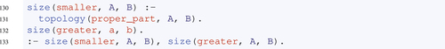
In Clingo2DSR, the evaluation of spatial relations is delayed by means of symbolic reasoning until they require numerical computations. Firstly, we use the algebraic properties of spatial relations to detect axiomatic spatial relations such as contact(C, C) where $\mathit{C}$ is any region. Secondly, we use the logical implications between spatial relations to deduce necessary spatial relations, for example, size(smaller, A, B) must hold if topology(proper_part, A, B) holds.

By alternating between these two steps, we populate the knowledge base with symbolically derived spatial relations. An incomplete ASP encoding is shown below. In particular, we express that contact is reflexive, discrete and partial_overlap are symmetric, pp (proper part) is transitive, and pp implies smaller.

Clingo2DSR encodings If spatial relations are not derived from symbolic reasoning, they can require various degrees of numerical evaluations. In some cases, numerical evaluations can be shortcut by necessary conditions that are less costly to compute, e.g. two polygons are discrete if their axis-aligned bounding boxes (AABBs) are discrete.

In Clingo2DSR, we use dictionary _aabbs to map spatial objects to their AABBs, so we can compare the minimum and maximum coordinates between two AABBs as a preliminary step to evaluating the exact topological relation between two spatial objects. This enhances the GDB with general spatial data structures (detailed in Subsection 6.3) to shortcut computationally expensive evaluations.⁸

In other cases, the GDB invokes external libraries and solvers to compute spatial relations. In Clingo2DSR, binary spatial relations are encoded as theory atoms of the form $\{\mathit{id}1,\mathit{id}2\}$ where $\mathit{p}\in \{\mathit{size},\mathit{incidence},\mathit{topology}\}$ and id1 and id2 are object IDs in symbolic ASP. If $\mathit{id}1$ and $\mathit{id}2$ have fully-ground geometric representations, the GDB retrieves their geometry IDs, and computes the spatial relation $\mathit{rel}$ over their corresponding shapes. This appends a new key-value pair $(\mathit{id}1,\mathit{id}2):\mathit{rel}$ to the dictionary _rels, and adds a new predicate $\mathit{p}(\mathit{rel},\mathit{id}1,\mathit{id}2)$ to symbolic ASP.

In very special cases, spatial relations such as incidence or topology can be translated into a stack of polynomial constraints and solved (i.e. decide if the constraints are jointly satisfiable) in an external SMT solver such as Z3 (Walega et al., 2015, 2017). For example, the incidence relation inside between a point and a convex polygon is translated into a system of constraints stating that the point should be left of every counter-clockwise-oriented boundary edge of the polygon.

In $\mathit{Z}3$, algebraic numbers⁹ such as $\sqrt{2}$ and $\frac{1}{7}$ can be represented without floating point approximations, so spatial relations can be evaluated without rounding errors. This enhances the GDB with real arithmetic solving capabilities (detailed in Subsection 6.4) to compute mathematically rigorous spatial relations.

5.3. Spatial functions

Let $D_1,\dots ,D_n$ be spatial domains. A spatial function $\mathit{f}$ of arity $(\mathit{n}-1)$ maps spatial objects $o_1,\dots ,o_{\mathit{n}-1}$ such that $o_i\in D_i$ for $1\le \mathit{i}\le (\mathit{n}-1)$ to a single spatial object $o_n\in D_n$. For example, if shift is the linear translation function, $\mathit{v}$ is a vector $(5,5)$ and $\mathit{T}$ is a polygon with vertices $((0,0),(10,0),(5,5))$ then $(\mathrm{shift}\mathit{Tv})$ evaluates to the polygon with vertices $((5,5),$ $(15,5),$ $(10,10))$.

Spatial functions vary by arity (unary, binary, and variadic) and can be categorized into metric functions (extent, centre, aabb, distance, offset), linear transformations (shift, scale, rotate, flip), and Boolean operations (union, intersect, difference) (Kyzirakos et al., 2012).

Moreover, spatial functions can require external arguments (rotate by an angle or offset by a distance) and they can range over multiple spatial domains (the intersection of two regions can be a point, a line segment, or a region).

For consistency, we consider the set of real numbers $\mathbb{R}$ as a de facto spatial domain to define spatial functions with numbers as external arguments. Furthermore, we introduce a void spatial entity to ensure that spatial functions are closed over spatial domains. For example, the intersection of two disconnected polygons (i.e. no common interior points) is not a polygon itself, but the void spatial entity.

In Table 1, we provide formal encodings for a selected list of spatial functions using ASP theory atoms. For brevity, we use variables (e.g. $\mathit{Region}$, $\mathit{Point}$) to denote the type of theory atom elements ($\mathit{t}$) and guards ($\mathit{c}$).

Clingo2DSR encodings Spatial functions are encoded using ASP theory atoms with the theory operator “$=$” (see Lines $39$-$43$). That is, $\{\mathit{t}\}=\mathit{c}$ signifies that the result of applying function $\mathit{f}$ to $\mathit{t}$ is equal to a constant $\mathit{c}$ where $\mathit{t}$ is a spatial theory term consisting of a list of spatial objects with predefined connectives such as “$\ast$”, “$\mathit{n}$”, “$+$”, and “—” (see Lines $34$-$38$).

In the following, the function difference is called when the theory atom &diff{id1-id2}=c_diff becomes ground. The function retrieves the geometry IDs of $\mathit{id}1$ and $\mathit{id}2$, computes the difference between their corresponding shapes, and constructs a new geometry ID by concatenating the functor name and the two geometry IDs, i.e. “diff(geom_id1,geom_id2).”

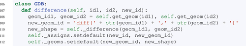
During this step, the new shape is mapped to the new geometry ID via _geoms, and the new geometry ID is mapped in _assigns to the object ID in symbolic ASP denoting the resulting difference, i,e. c_diff.

6. Geometry database

As demonstrated in Section 5, the GDB constructs shapes from an external geometry database _repr, to create an internal geometry database _geoms that maps symbolic IDs of BIM objects to their geometric representations. Then the GDB updates this internal database with new spatial entities and relations that are the results of spatial functions and relations, evaluated in sync with ASP model search.

In this way, the GDB ensures a bi-directional data flow between the logic program and numerical data and computations. On one hand, the Spatial Propagator (SP) translates theory atoms into spatial functions and relations over spatial entities, and sends them to the GDB for numerical evaluation. On the other hand, the GDB performs spatial calculations and sends the results back to the SP, to continue theory propagation.

During the numerical evaluation in the GDB, new spatial entities are created, e.g. the union of two polygons, and new relations are derived, e.g. the topology between two polygons. This knowledge is communicated to the SP to 1) ground new theory atoms that depend on the new spatial entities, 2) check spatial constraints involving the new spatial relations.

However, several practical difficulties persist in maintaining a dynamic and consistent link between state-dependent computations and a symbolic logic program. In the following, we propose a series of optimization techniques in the GDB to address the specificity of DSR tasks in a declarative reasoning framework such as ASP.

Optimisation features Firstly, variadic spatial functions such as union are applied over a set of spatial entities, which is subject to heuristics in ASP grounding. In Subsection 6.1 we demonstrate a minting service for generating unique geometry IDs that denote the results of spatial functions to avoid redundant computations.

Secondly, a set of theory atoms have implicit dependencies so they need to be ground in a specific order such that a spatial function or relation is computed only if all of its arguments are ground. This contradicts the declarative character of ASP and can lead to slow grounding times and in an adverse case, grounding inconsistencies. In Subsection 6.2, we redefine the semantics of theory atoms using nogood constraints so they must be derived from the logic program, to provide on-demand grounding.

Thirdly, spatial relations can be shortcut by necessary conditions that are less costly to evaluate. In Subsection 6.3, we build internal spatial data structures in the GDB with attributes _exts and _aabbs, to perform a preliminary assessment of spatial relations given the spatial entities’ extents (area or volume) and bounding boxes.

Fourthly, some spatial relations can be translated into constraint satisfiability problems. In Subsection 6.4, we use the SMT solver $\mathit{Z}3$ to derive the exact spatial relations based on real arithmetic, to circumvent numerical instability issues.

6.1. Geometry IDs

Consider the following Clingo2DSR rulebase. The (head) theory atom in Line $114$ is a fact, thus included in the initial model assignment. The ground form of this atom, &union{s5; s10; s52} is obtained by binding variable S with the object IDs of slab elements.

When the ground theory atom is sent to the GDB to compute the union, we sort the list of object IDs by the following spatial term ordering rules.

• 1. $\mathit{t}$ $\prec$ $\mathit{u}$ for integer $\mathit{t}$ and string $\mathit{u}$

• 2. $\mathit{t}$ $$ $\text{}\mathit{nu}$ for integers $\mathit{t}$ and $\mathit{u}$ if $\mathit{t}$ $\le$ $\mathit{u}$

• 3. $\mathit{t}$ $$ $$ for strings $\mathit{t}=\mathit{f}(t_1,\dots t_m)$ and $\mathit{u}=\mathit{g}(u_1,\dots u_n)$ if

(a) $\mathit{f}\prec \mathit{g}$ according to the lexicographical ordering of functors, e.g. buffer $\prec$ intersect $\prec$ union

(b) there exists $\mathit{i}$ such that $t_i{u}_i$ and for all $\mathit{k}<\mathit{i}$, $t_k=u_k$

(c) $\mathit{m}<\mathit{n}$ and for all $\mathit{k}\le \mathit{m}$, $t_k=u_k$

This produces a sorted list $[\mathit{s}10,\mathit{s}5,\mathit{s}52]$. We then construct the shape of each slab element, which generates a list of integer geometry IDs, e.g. $[1,2,3]$. We union the shapes to produce a new spatial object. This spatial object has a symbolic ID union(slab), ie. the theory guard, and is assigned a concatenated geometry ID, $``\mathit{union}(1,2,3)$, that embeds the rationale behind the spatial operation, i.e. the functor name and the sorted arguments.

This avoids redundant computations of variadic functions such as union and intersect, as &union{s5; s10; s52} and &union{s10; s52; s10} yield the same result by associativity and commutativity. In ASP, both expressions can occur during grounding. Therefore, our minting service ensures that the diverging ground forms of theory atoms is deterministically mapped to a unique geometry ID, independent of the order in which theory terms are grounded, so they can be invoked without any computations in future solving steps.

6.2. Cascading spatial computations

Consider the functional space of a bathroom object, which are regions in which a person must be located to use the bathroom object. In architecture literature, the shape of this functional space depends on the category of bathroom object (Figure 7).

Figure 7. 2D footprints of functional spaces of common bathroom objects. Taken from (Neufert et al., 2000).

Geometrically, the functional space can be computed by first scaling then shifting the bounding box of the bathroom object. The parameters for scaling and shifting are encoded as follows. These facts are maintained in a custom module called “neufert” (i.e. an external clingo file named “neufert.lp”), to indicate the evidence-based provenance of the specified parameters.

In Clingo2DSR, the above facts are used in conjunction with theory atoms to derive functional spaces. First, we compute the bounding box of a bathroom object b9 ($119$). Then, we scale it by a factor of $1.2$ (Lines $120$-$122$). Finally, we shift it by a distance of $0.2\mathit{m}$ (Lines $123$-$125$). In addition, we use the statement #include to invoke the module “neufert.lp” to ground variables S and T.

During default ASP ground-and-solve, theory atoms can have defined or external semantics, i.e. they do not have to be derived from the logic program. As a result, a theory atom in a rule body can become True, despite its theory terms (e.g. spatial object, scaling parameter) not being ground. In a classical “guess-and-check” ASP program, the scaling parameter can take a range of numeric values depending on the scenario (encoded as choice rules), while some scenarios are inconsistent with available information about a building (encoded as integrity constraints). This can lead to prohibitively slow grounding times as ASP.

To circumvent these issues, we propose to 1) encode the dependencies among theory atoms as rules, 2) discriminate and match head and body theory atoms, and 3) add clauses to SP so matching head and body theory atoms are logically equivalent. In the above example, the function scale is applied over the result of the function aabb, i.e. (bb(b9)). We express this dependency with the rule in Lines $120$-$122$, where the theory atom &scale is the rule head and the theory atom &aabb is in the rule body.

In Clingo2DSR, the above logic program is first parsed and transformed in the PAT to add location arguments to theory atoms, e.g. Lines $119$-$125$ become:

In this ground program, $\mathit{aabb}(\mathit{head})\left\{\mathit{b}9\right\}=\mathit{bb}(\mathit{b}9)$ and $\mathit{aabb}(\mathit{body})\left\{\mathit{b}9\right\}=\mathit{bb}(\mathit{b}9)$ constitute a matching pair of theory atoms as they have the exact same theory elements and only differ by the location. Assuming they are given the solver literals $l_h$ and $l_b$, we add two nogood constraints $\{l_h,\mathrm{\neg }{l}_b\}$ and $\{\mathrm{\neg }{l}_h,l_b\}$ to the SP during initialization.

This makes the literals logically equivalent as one is True if and only if the other is True. Therefore, $\mathit{aabb}(\mathit{body})\left\{\mathit{b}9\right\}=\mathit{bb}(\mathit{b}9)$ becomes True when and only when $\mathit{aabb}(\mathit{head})\left\{\mathit{b}9\right\}=\mathit{bb}(\mathit{b}9)$ is derived, thus establishing an implicit execution order among program rules.

In a solving step, propagated literals are evaluated recursively by first identifying theory atoms whose elements do not exist as guards to some other theory atoms. In Algorithm 1, a set of declaratively defined theory atoms is organized into a cascade.

Table

Algorithm 1 Compute spatial functions.

In this way, we ensure that an unordered set of deductive rules always fires in the expected order. For functional spaces, this means that first the bounding box is calculated, then scaled, and finally, shifted.

6.3. Spatial data structures

Consider the theory atom $\mathit{aabb}/1$ in Line $119$. When this atom becomes ground, the GDB constructs the geometry of b9, computes its AABB as a tuple of coordinates (xmin, xmax, ymin, ymax), and updates the internal attribute _aabbs. When the spatial function aabb is applied to a spatial entity, the theory atom can retrieve its AABB from the GDB without any computation, as the spatial entity has been previously added to the GDB (otherwise the theory atom would not be evaluated).

In Clingo2DSR, attributes _aabbs and _exts provide spatial data structures by means of arithmetic comparisons. To give an example, if we want to check the topology relation between two polygons a and b, we can retrieve their areas via _exts from the GDB, compare them, and eliminate spatial relations equal and proper part if the area of a is greater than the area of b.

More generally, the evaluation of spatial relations such as topology can often be shortcut by necessary and sufficient conditions stemming from simple numeric comparisons which are less costly than evaluating the exact spatial relation in SMT solvers.

To give an example, the size relation smaller is a necessary condition to the topology relation proper_part, so that the negation of smaller is sufficient to determine that proper_part does not hold. In Clingo2DSR, we encode the necessary condition as a deductive rule in Lines $130$-$131$. The size relation in Line $132$ is automatically added as the GDB constructs $\mathit{a}$ and $\mathit{b}$ and compares their size. In Line $133$, we use an integrity constraint to force size(smaller, a, b) to be False. As a result, we can deduce that topology(proper_part, a, b) must not hold.

Similarly, the topology relation disconnected between two spatial entities can be shortcut by the topology relation between their bounding boxes (see Figure 8). The latter consists of four arithmetic comparisons in case of 2D regions, which is significantly more computationally economic than solving a system of polynomial constraints. In the following, we showcase one example where the topology relation between two polygons can be determined by comparing the integer coordinates of their AABBs.

Figure 8. Deducing topological relations disconnected between two regions a and B by comparing their bounding box coordinates.

6.4. Evaluating spatial relations with SMT solvers

If spatial data structures fail to determine spatial relations, we then use SMT solvers as a last resort to determine mathematically rigorous spatial relations. That is, the GDB translates spatial relations into a stack of polynomial constraints and solves it in an external SMT solver.

SMT solvers contrast numerical solvers that use floating point representations. Consider the point $(\frac{1}{\sqrt{2}},\frac{1}{\sqrt{2}})$ and a unit circle centered at $(0,0)$. The point is exactly on the boundary of the circle. However, a floating point representation will locate the point either slightly inside or outside of the circle (depending on how rounding is handled), contradicting the reality.

Computational geometry libraries such as GPC and PyMesh use floating point representations to perform Boolean clipping on polygons and polyhedrons, and raise similar numerical instability issues due to rounding errors (Li et al., 2019). In contrast, SMT solvers such as $\mathit{Z}3$ (De Moura & Bjørner, 2008) are able to encode natively algebraic numbers and can give outputs without rounding.

In the following, we demonstrate a proof-of-concept implementation of integrating $\mathit{Z}3$ with Clingo2DSR for evaluating i) point-polygon incidence relation inside and ii) polygon-polygon topology relations overlap.

In Algorithm 2, the incidence relation inside between a 2D point and a simple convex polygon is translated into a system of constraints specifying that the point should be left of (as defined in $\mathcal{L}\mathcal{R}$ (Scivos & Nebel, 2005)) to all counter-clockwise-oriented edges of the polygon. If the inequalities are jointly satisfiable, we conclude that the point is inside the polygon.

Table

Algorithm 2 Determine (incidence) spatial relations.

This gives a straightforward characterization for the topology relation overlap between two convex polygons as defined in the DE-9IM (Egenhofer & Franzosa, 1991). Two convex polygons overlap if they have at least a common interior point. In Algorithm 2, if the inequalities are jointly satisfiable, we can use s.model() to get a witness, i.e. a common interior point.

DSR with unground geometry If spatial objects have partially ground or unground geometric representations, $\mathit{Z}3$ checks the satisfiability of a system of constraints over a mix of constants and variables. If the constraints are inconsistent, the GDB adds a nogood to theory propagation to check partial assignments. Otherwise, $\mathit{Z}3$ produces a witness, which grounds spatial objects with numerical configurations.

In the following, we use Clingo2DSR to encode a qualitative constraint network (QCN) where certain topological relations must hold between pairs of circles. This is achieved by a guess part which assigns spatial relations to pairs of spatial objects, and a check part that checks whether the assigned spatial relations are consistent with domain constraints and spatial theories.

In Line $140$, we use a choice rule to assign exactly one $\mathcal{R}\mathcal{C}\mathcal{C}$ −5 relation $\mathit{R}$ to all pairs of circles $(\mathit{C},\mathit{C}\mathrm{\_})$. In Line $141$, we use theory atoms of the form $(\mathit{R},\mathit{C},\mathit{C}\mathrm{\_})$ to translate spatial relations into polynomial constraints.

During initialization, the symbolic ID of a circle is mapped to a triplet of variables $\mathit{x},\mathit{y},\mathit{r}$ in a dictionary _vars, implemented as a shared class attribute between the theory propagator SP and the geometry database GDB.

During theory propagation, topology(R, C, C_) are deterministically assigned due to the choice rule in Line $140$ and the constraints in Lines $143$-$145$. The ground theory atoms are then sent to the GDB where they are translated into constraints over the circles’ center coordinates and radii. Z3 checks the satisfiability of the constraint store and transfers the results back to SP via the attribute _sat.

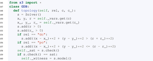
In the above problem, _sat is set to unsat, meaning that the total model assignment is unsatisfiable with respect to spatial theories. That is, there does not exist a configuration where $c_1$ is part of both $c_2$ and $c_3$, and $c_2$ and $c_3$ are disconnected. Thus, Clingo2DSR provides an operational system for deriving composition tables of spatial relations, by coupling a logic program with external SMT solvers.

7. Spatial theory solving

DSR tasks introduce an important challenge to theory enhanced ASP in that theory nogoods w.r.t. spatial theories cannot be fully defined in advance, but may be derived on the fly when 1) grounding theory terms with numerical data, and 2) propagating spatial theories with the results of numerical computations.

In the first case, if spatial theory expressions are substituted with numerical data wherever possible, this can lead to a combinatorial blowup of ground instantiations when only a small fraction are spatially consistent.¹⁰ In the second case, if learnt spatial constraints are not recorded during theory propagation, this can lead to branching in model search and result in unnecessary solving steps.

From a practical standpoint, DSR problems are often encoded as non-stratified programs where grounding and solving cannot be easily interleaved. However, spatial computations are naturally cascading, which provides a series of implicit decision points that enable on-demand grounding and solving.

In Clingo2DSR, we negotiate the above issues with 1) a transformed logic program to deduce consecutive solving steps, and 2) a modified ground-and-solve approach where the SP invokes the GDB at each solving step. The idea is to ground parts of the logic program needed for a solving step, compute the necessary spatial functions, and derive the necessary spatial relations. In the SpatialChecker (SP), the derived spatial relations are checked for consistency with respect to spatial theories in combination with domain constraints. If they are jointly satisfiable, then the computed spatial functions are sent back to symbolic ASP to ground new parts of the logic program needed for the next solving step.

In the following, we describe three building blocks that constitute our modified ground-and-solve approach. Firstly, we use Algorithm 3 Parse and Transform (PAT) to transform a logic program. This algorithm adds integrity constraints to variable check, adds facts and rules to the SP, and extends spatial theory atoms with location arguments.

Table

Algorithm 3 Parse and Transform (PAT)

Secondly, we use Algorithm 4 Spatial Propagator (SP) to propagate spatial theories. During initialization, we add symbolic atoms to the SC and ground SC with constraints in check. In addition, we force matching head and body theory atoms to always have the same truth value, i.e. $\mathit{aabb}(\mathit{head})\left\{\mathit{O}\right\}=\mathit{ab}(\mathit{o})$ and $\mathit{aabb}(\mathit{body})\left\{\mathit{O}\right\}=\mathit{ab}(\mathit{O})$ must be both True, or both False, in a model assignment. This is achieved by adding nogoods $[\mathit{head},-\mathit{body}]$ and $[-\mathit{head},\mathit{body}]$ where head and body, respectively, denote the solver literals of head and body theory atoms.

This encoding is designed to circumvent the bifurcating interpretations of theory atoms, namely, whether they must be derived through ASP rules (defined or external) and whether a theory constraint only holds when its corresponding theory atom is True (strict or non-strict) Gebser et al., 2016.

We use these nogoods to ensure that theory atoms can only be derived through the logic program (defined) and spatial computations are only carried out when their theory atoms become True (non-strict). In this way, state-dependent spatial computations are organized into a cascading stack and evaluated in solving steps where their associated theory atoms are derived from the logic program.

Table

Algorithm 4 Spatial Propagator (SP)

During unit propagation, we perform a first consistency check in the SC with literals in the current model assignment as assumptions. If this returns satisfiable, we compute spatial functions and derive spatial relations. Then, we perform a second consistency check in the SC with new predicates constructed from derived spatial relations in the GDB. If this returns unsatisfiable, the conjunction of current decision literals is recorded as a nogood, which forces the SP to backtrack. Otherwise, the propagation continues until reaching a total assignment. In this way, we ensure that partial assignments are consistent before they are propagated any further.

Thirdly, we use the Spatial Checker (SC) to check spatial consistency in partial model assignments. First, integrity constraints under the #check directive are identified during parsing and added to a builder object, which is used to ground the base program of SC. Then SC performs satisfiability checks with additional assumptions from partial models assignments during theory propagation. The interactions between SP, GDB, SC, and PAT are shown in Figure 2.

Clingo2DSR is implemented via clingo’s Python API. As shown below, we customize the Application class to ground and solve a logic program w.r.t background spatial theories. Firstly, we import “spatial.py” as a Python module which contains class definitions for PAT, SC, SP, and GDB. Secondly, we parse the logic program and transform it so that theory atoms are augmented with location arguments. During this transformation, we use a variable check to collect integrity constraints under the program directive $\#\mathit{check}$. This variable is then used in the SP to ground the SC with constraints which is called upon partial assignments.

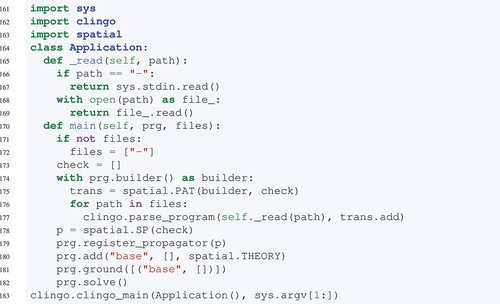
In this way, an ASP program is parsed and interpreted according to spatial theory atom definitions, then grounded and solved during theory propagation by invoking the GDB which retrieves numerical data and performs numerical computations.

8. Empirical evaluation and demonstrative case studies

The purpose of this section is (a) to empirically evaluate Clingo2DSR on two scalability experiments to assess the impact on runtime of the GDB and the relative runtimes in the stages in the computational pipeline, thereby addressed research question RQ1, and (b) to demonstrate the diversity of important tasks that Clingo2DSR can be used for in the domain of architecture and construction, and to demonstrate that Clingo2DSR can run fast enough in practice on large, real-world BIM models.

As described in previous sections, Clingo2DSR natively supports DSR tasks by seamlessly integrating a rule-based inference engine with spatial computations. This is done by enhancing ASP with general spatial axioms and calculi, to interpret and evaluate spatial functions and relations.

However, real-world DSR tasks often allude to implicit domain-specific knowledge. In BIM models, knowledge about buildings can pertain to constructibility, e.g. “every building component needs to be transitively supported by the foundation.” In ASP, this knowledge can be expressed as mixed possibilities (such that a wall can be constructed at any timepoint) and constraints (such that the wall cannot be constructed before its supporting slab).

Furthermore, BIM models are often riddled with imprecise semantics and inaccurate geometric details. For instance, the IFC relation IfcRelConnectsElements does not discriminate between cases where two elements are physically or logically connected. This motivates the use of default reasoning, to assume that a wall (topologically) meets flush with a slab when the relation holds between them.

On the other hand, the exact geometric details might not support the relation contact due to numerical approximations. This motivates the use of hypothetical reasoning, to abduce that the relation must hold between a wall and its supporting slab, based on our observation that the building is structurally valid and our domain knowledge that a wall cannot be free floating.

This section demonstrates the use and performance of Clingo2DSR with large, complex BIM models. We present the algorithmic and operational aspects of Clingo2DSR with three typical DSR tasks, each demonstrating one key feature of Clingo2DSR when applied to real-world applications:

• code compliance assessment, where we demonstrate how Clingo2DSR uses default reasoning and hypothetical reasoning to assert and retract information based on domain knowledge (Subsection 8.2)

• construction safety analysis, where we demonstrate how Clingo2DSR deals with numerous timesteps in 4D BIM models with choice rules (Subsection 8.3)

• renovation decision-support, where we demonstrate how Clingo2DSR deals with spatially inconsistent solutions with constraint-driven solving (Subsection 8.4)

With respect to runtime performance, we are yet to undertake a comprehensive scalability analysis that compares Clingo2DSR with other systems such as CLP(QS) (Bhatt et al., 2011; Schultz & Bhatt, 2014, 2015), ASPMT(QS) (Walega et al., 2015, 2017) or the DLV system (Calimeri et al., 2020), and thus leave this for future work.

8.1. Empirical evaluation

In this subsection we present two empirical experiments that assess the impact on runtime performance of the features in our new Clingo2DSR system compared to our previous systems that did not have these features (Li, Fitzgerald, et al., 2022; Li, Teizer, et al., 2020), namely implementing spatial functions using theory atoms combined with a dedicated geometry database.¹¹

Each experiment consists of a set of $\mathit{n}$ input polygons, and applies boolean operations to subsets of the input. The shape of the input polygons is illustrated in Figure 9. In a given experiment with $\mathit{n}$ polygons, each polygon $\mathit{i}$ (for $1\le \mathit{i}\le \mathit{n}$) consists of $\mathit{m}$ “teeth” across the upper side, and the lower left vertex is the coordinate $(\mathit{i},\mathit{i})$. The length of each polygon is $100\text{cdotm}$ and the height is $200$. Thus, the vertex count of each such polygon is $2\mathit{m}+3$.

Figure 9. Shape of the $\mathit{i}$th input polygon in the empirical experiments, for $1\le \mathit{i}\le \mathit{n}$.

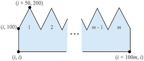
The input polygons are crafted so that the complexity with respect to the vertex count can be scaled up in a simple systematic way. The polygons are arranged to ensure that (a) no two polygons have an identical set of vertices, and (b) that no pair of polygons is disconnected (i.e. all pairs of input polygons share a subset of interior points).

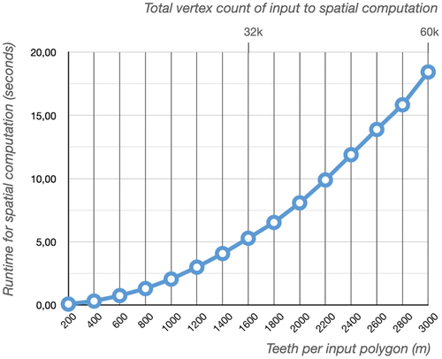
In the first experiment we sought to determine the relative runtime required in four stages of the computational pipeline when the program consists of a single spatial computation. The four stages we measured are as follows: the initial loading time for the geometry database; grounding; solving (total); geometry computations during solving (which includes the time required to query the GDB and the time required to execute spatial functions). We fixed the number of polygons $\mathit{n}=10$ and increased the number of teeth per polygon $\mathit{m}$ in increments of $200$, from $200$ to $3000$.

The program consists of a union operation of all $10$ input polygons:

The results are plotted in Figure 10; the spatial computations dominate as $\mathit{m}$ increased, taking above $95\mathrm{\%}$ of the solving time for $\mathit{m}\ge 200$, and thus the plot in Figure 10 only shows the spatial computation time. The runtime results of the smallest test ($\mathit{m}=200$) and the largest test ($\mathit{m}=3000$) are presented in Table 2. Taking the union of $10$ polygons each with $\sim 6\mathit{k}$ vertices took approximately $18.46$ seconds, with $18.43$ spent on computing the union of the geometries.

Table 2. Runtime (seconds) of four stages for $\mathit{m}=200$ and $\mathit{m}=3000$ in experiment 1.

m	Loading GDB	Grounding	Solving (total)	Spatial computations during solving
200	0.0231	0.0013	0.0801	0.0773
3000	0.0171	0.0001	18.4616	18.4317

Figure 10. Plot of experiment 1 comparing input size $\mathit{m}$ (teeth per polygon) with computational runtime of spatial computation, for fixed number of polygons, $\mathit{n}=10$.

In the second experiment we sought to assess runtime performance when storing the results of applying spatial functions and returning these results when the same functions are applied on the same input arguments, analogous to tabled execution and memoization. This experiment serves to assess the runtime performance of our new system Clingo2DSR compared to our previous systems that implemented spatial computations via external functions and built-in aggregates (Li, Fitzgerald, et al., 2022; Li, Teizer, et al., 2020).

We chose to use polygons with a small number of vertices so that each spatial operation between pairs of polygons would not be computationally demanding, and crafted the ASP program to have a high number of answer sets with many repeated spatial function calls being applied to the same input arguments. Therefore, we fixed the vertex complexity of the polygons to $\mathit{m}=10$ teeth per polygon (corresponding to 23 vertices per polygon), and increased the number of polygons from $5$ to $30$ in increments of $5$.

The program consists of $\mathit{n}$ polygons. A choice rule selects exactly two pairs of distinct polygons with the predicate $\mathit{a}/2$. A spatial function call then takes the difference between the polygons in each pair:

We ran the set of experiments with the store feature turned off (i.e. without memoization, which simulates our previous systems that did not have this feature (Li, Fitzgerald, et al., 2022; Li, Teizer, et al., 2020)) and again with the store feature turned on. We measured the total solving time (seconds), the time spent applying the spatial functions (seconds, which includes GDB query time and spatial function computation time), and the number of times that the difference spatial operation was executed.

The results (presented in Table 3) show a runtime improvement of the spatial computing time by an order of magnitude for $\mathit{n}\ge 10$, and a reduction in spatial computations of between 2 and 4 orders of magnitude for $\mathit{n}\ge 10$. We argue that this demonstrates two significant advantages of managing geometric data and spatial functions in a dedicated geometry database (i.e. advantages of our new Clingo2DSR system over our previous systems).

Firstly, spatial computations can be memoized, which improves runtime performance when spatial functions are applied repeatedly on the same input arguments over many answer sets. In Experiment 2 we intentionally avoided computationally demanding spatial functions (i.e. we selected $\mathit{m}=10$ for all polygons), and thus we can expect a yet greater improvement in performance when, for example, generating 3D visibility volumes (Krukar et al., 2020).

Secondly, we argue that this experiment demonstrates the performance benefits of avoiding redundant spatial function applications, thereby further motivating the value of implementing spatial computations via theory atoms, in contrast to (for example) external functions processed by the grounder, as we implemented in our previous systems (Li, Fitzgerald, et al., 2022; Li, Teizer, et al., 2020). To highlight the issue, we present the following clingo program that defines an external function $\mathit{sum}/2$ that adds two integers together. A predicate $\mathit{result}/4$ applies a nested call to sum in order to add three integers together, the values of which must be the argument of a fact $\mathit{p}/1$. The three numbers $\mathit{A},\mathit{B},\mathit{C}$ must be larger than some arbitrary number defined in predicate $\mathit{g}/1$, which we specify so that there is exactly one answer set for the program, and so that only the largest three values in $\mathit{p}$ facts are the solution for $\mathit{A},\mathit{B},\mathit{C}$, respectively.

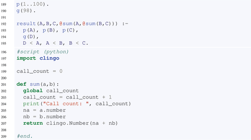
In searching for the answer set, the function $\mathit{sum}$ is executed $4950$ times, despite there only being one substitution for $\mathit{A},\mathit{B},\mathit{C}$ that satisfies the body of the rule defining the $\mathit{result}/4$ predicate. That is, some $4948$ of the calls to $\mathit{sum}$ are redundant and could be avoided, which would have a significant impact on performance if $\mathit{sum}$ was a more computationally demanding spatial function (e.g. union, etc.) applied over large, complex geometries. Thus, theory atoms, combined with a dedicated geometry database, provide powerful mechanisms necessary for controlling and managing spatial function calls.

Table 3. Results of experiment 2 comparing number of polygons ($\mathit{n}$) given as input to the experiment 2 ASP program with the solving and spatial runtimes, and the number of spatial function applications, with and without the GDB feature of storing and retrieving spatial computation results.

		n
Store		5	10	15	20	25	30
No	Total solving time (sec)	0.02	0.42	3.10	14.32	49.33	137.18
	Spatial computing time (sec)	0.02	0.27	1.44	4.80	12.13	25.58
	Spatial operation count	792	16192	88192	288793	719992	1513793
Yes	Total solving time (sec)	0.01	0.17	1.76	9.76	38.04	112.80
	Spatial computing time (sec)	0.00	0.02	0.11	0.39	1.07	2.29
	Spatial operation count	20	90	210	380	600	870

8.2. Code compliance assessment

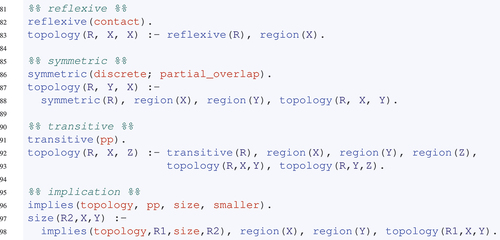
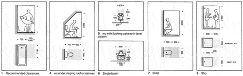
We demonstrate the use of Clingo2DSR for code compliance assessment tasks with the following requirements from the NZBC.

R1. (NZBC-D1.7.0.3) Accessible doors shall have at least 760 mm clear opening.

R2. (NZBC-D1.1.4.1) Access route shall have a height clearance of minimum 2100 mm.

R3. (NZBC-D1.2.2.1) The clear width of an accessible route shall be not less than 1200 mm.

R4. (NZBC-D1.7.0.1) Where doors open into a lobby, the clear space between open doors shall comply with Figure 11.

R5. (NZBC-G1.6.1.1) There shall be no direct line of sight between an access route or accessible route and a WC, urinal, bath, shower, or bidet.

Figure 11. Minimum clearance requirements between successive doors on access routes. Taken directly from (Department of Building and Housing, 2011).

Default reasoning By definition, accessible route is a subclass of access route.¹² We can assume, by default, that an access route is an accessible routes unless we can prove that it is not. In Clingo2DSR, this is expressed as a base rule:

The defeating fact -accessible_route(R) is True if i) R is not connected to at least one accessible door (deduced by default reasoning from R1), 2) R does not have a minimum height clearance of 2.1$\mathit{m}$ (R2), and so on. In Clingo2DSR, these exceptions are encoded as deductive rules. We use aggregate #count to denote lower bounds (e.g. at least one).

This encoding allows us to add defeating facts without modifying the base rule. In this way, we can easily revise our assumption by adding exceptions so the base rule applies when none of the exceptions are True, otherwise the base rule is exempt from applying.

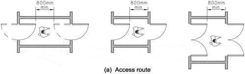
Hypothetical reasoning In a BIM model, a door might be missing information about its hinge side (left or right) or swing direction (in or out). This information is crucial to determine whether a door intrudes the clear space of an access route when opened. Moreover, R4 requires that access routes must have a minimum clearance of 800mm between opening doors (see Figure 11).

In Clingo2DSR, we encode hypotheses about a door’s swing direction and hinge side as choice rules. This generates four models where a door either swings inwards or outwards and the hinge is located on either the left or right side of the door panel.

First, we compute the operational space of a door, regions required for its operation (e.g. swinging), as a quarter circle based on the door’s swing direction and hinge side.

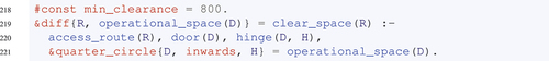
If a door swings into an access route, we subtract the door’s operational space from the access route using theory atom &diff in Lines $220$-$222$. The resulting geometry is identified in symbolic ASP by the object ID clear_space(R) where R denotes the access route.

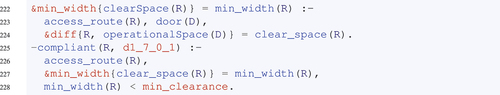
Finally, we compute the minimum width of this clear space as min_width(R). If this minimum width is less than 800mm, we deduce that R4 is violated.¹³

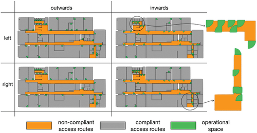
Figure 12 shows the floor plan of the ground level in Christchurch City Council, a two-storey building in New Zealand. In the right column, we assert that all doors swing inwards, which entails multiple violations as a number of doors clash when opened.¹⁴ However, the building consenting officer observes that none of the doors collide during operation, thus we retract both hypotheses as they contradict known facts.

Figure 12. Operational spaces of doors (green regions) and access routes (compliant as gray regions and non-compliant as orange regions) in four distinct scenarios alternating the swing direction and the hinge side.

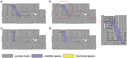
Runtime performance An alternative interpretation of R5 is that the functional space of bathroom objects (described in Subsection 6.2) also needs to be visually excluded from access routes. This is formalized into a guess part where every pair of access route and visibility space is sent to the GDB to derive their topology relation, and a check part that deduces violation if the derived spatial relation is overlap. For brevity, we use functional_space/2 and visibility_space/2 to denote theory atoms.

We execute the formalized rules w.r.t a two-storey building in Christchurch, New Zealand. The BIM models contains 8304 objects, of which 12 are bathroom objects. We run Clingo2DSR directly from the command line by invoking the clingo file containing formalized rules. Clingo2DSR identifies four non-compliant bathroom objects whose functional space can be seen from an access route (see Figure 13).

Figure 13. Privacy violations in the NZ building. Functional spaces, visibility spaces, and access routes are, respectively, denoted as yellow, purple and gray regions.

Table 4 shows the runtime performance of Clingo2DSR for checking code compliance against large-scale buildings. For R5, Clingo2DSR generates 132 visibility spaces and 38 movement spaces and check their pair-wise topology in an average runtime of 1.6 seconds.

Table 4. Model statistics and runtime performance of Clingo2DSR for checking code compliance on real-world buildings.

Code provisions	Model statistics	Runtime	Reference documents
There shall be no direct line of sight between an access route or accessible route and a WC,urinal, bath, shower, or bidet.	Two-storey building in New Zealand with 8304 BIM objects	1.6 seconds	NZBC-G1-6.1.1
Where doors open into a lobby, the clear space between open doors shall comply with Figure 27.	12.5cmTwo-storey building in New Zealand with 6796 BIM objects	8.4 seconds	NZBC-D1/AS1–7.0.1
The clear width of an accessibleroute shall be no less than 1200 mm.		0.3 seconds	NZBC-D1/AS1–2.2.1
Access route shall have a heightclearance of minimum 2100 mm		0.2 seconds	NZBC-D1/AS1–1.4.1

8.3. Construction safety analysis

The Occupational Safety and Health Administration (OSHA) (Safety & Administration, 2015) requires that leading edges that are 1.8 m or higher above a lower level must be protected by personal fall arrest systems. In our formalization of this rule, fall protection measures (e.g. guardrails) are needed in hazard spaces, geometrically modeled as the intersection between movement spaces (regions reachable by a person) and fall spaces (regions from which a person can fall by a dangerous distance) (see Figure 14).

Figure 14. 1) a person working from heights, taken directly from (der Bauwirtschaft (BG BAU), 2021). 2) movement spaces, fall spaces, and hazard spaces in a building under construction.

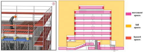
In a building under construction, leading edges are changing over time as the result of successively erected building components (e.g. movement spaces are growing). This is reflected in a construction plan that assigns a timepoint to every building component in a way that satisfies constructibility requirements.

In a construction plan, a building component, represented by a unique ID, belongs to a construction task, which has a start time $T_s$ (construct/2) and a duration $T_d$ (duration/2). We can then derive the component’s timestep $T_e$ (timestep/2) at which it is fully constructed.

In a 4D BIM model (i.e. a sequence of BIM models at successive timepoints), each building component has a type (is_a/2), and is contained in a building storey. In ASP, we use predicate timepoint/1 to define all possible timepoints in a construction plan. We then use a choice rule to assign a distinct timepoint to each ASP model with time_now/1. In each ASP model, we can derive all components that are constructed at the assigned timepoint with exists/3.

For each storey, we can union components of the same type that are contained in the storey using &union. This generates numerous spatial aggregates, to denote the union of slabs, columns, walls, opening, and so on, on each storey at a given timepoint.

In the next step, we use these theory atoms to derive movement spaces by subtracting floor-intersecting obstacles (walls subtracted by openings) from walkable surfaces (slabs subtracted by columns). To get around geometric discrepancies, we slightly buffer the unions by 0.01 m prior to Boolean operations. For simplicity, let the buffered union of slabs form a new region called “walkable,” and the buffered union of walls “obstacle.”

We then compute movement spaces as the difference between “walkable” and “obstacle” as follows:

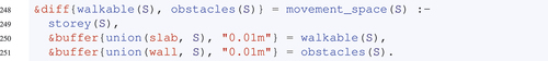
For each storey, fall spaces are computed as the difference between the site and movement spaces. In our formalization, the site is modeled as the bounding box of all constructed surfaces (slabs, columns, walls), buffered by 1$\mathit{m}$.

By definition, movement spaces and fall spaces are externally connected (touching at boundaries), so their intersection is comprised of line segments. As fall protection measures are typically installed inside movement spaces with some distance to leading edges, we buffer fall spaces by 0.5$\mathit{m}$ and compute their intersection with movement spaces as (fall) hazard spaces.

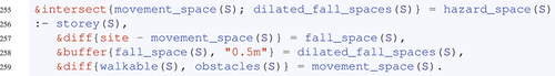
Runtime performance The above DSR problem is solved with respect to a 13-storey building with 282 BIM objects and a construction plan with 122 timepoints (see Figure 15). The semantic data (object type and relations) is extracted from the BIM model and converted to ASP facts. The geometric data (e.g. 3D meshes) is formatted into string representations and stored as key-value pairs in a text-based file. The geometry database constructs shapes of BIM objects when they are needed for grounding spatial theory atoms.

Figure 15. 1) The 13-storey building at timepoint 73 (The second slab quadrant on the second floor is about to be constructed). 2) The generated SVG outputs showing hazard spaces as red regions at time point 73 (a) and at timepoint 75 (b) when the fourth slab quadrant is placed.

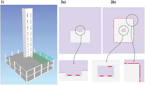
Clingo2DSR computes 184 spatial artifacts (movement spaces, fall spaces, and hazard spaces) per timepoint, and writes their 2D footprints to SVG files (see Figure 15b). Clingo2DSR performs a total of 301 unions, 45 buffering, 21 differences, and 44 intersections. The average runtime for a single Clingo2DSR call (which generates 122 models) is 2.28 seconds.¹⁵

Table 5 shows the operational performance of Clingo2DSR in executing construction safety analysis tasks against large-scale BIM models. The runtime has significantly improved for reasoning about 4D BIM models with numerous timepoints using theory extensions, compared to incremental solving (Gebser et al., 2019).

Table 5. Model statistics and runtime performance of Clingo2DSR for construction safety analysis on real-world buildings.

Code provision	Model statistics	Runtimes	Reference document
Each worker constructing a leadingedge 6 feet or more above a lower level must be protected by guardrailsystems, safety net systems, or personal fall arrest systems.	9-storey building in Germany with 5415 BIM objects	0.59 seconds	42cmOSHA 29 CFR 1926.501(b)(2)*
	Four-storey building in Denmark with 707 BIM objects	0.24 seconds
	Two-storey fire station in Germany with 1273 BIM objects	0.2 seconds
	Thirteen-storey building in Denmark with 259 objects	2.28 seconds for 122 timepoints

8.4. Renovation decision support

A renovation scenario is a set of building objects (such as wall and door), each object assigned one or several approaches (such as replace), and each approach assigned one or several features (such as translate). Renovation measures can entail spatial changes (such as shifting or resizing a door). These spatial changes can compromise spatial validity (such as the displaced door is no longer contained in its hosting wall).

In Clingo2DSR, we use choice rules to generate a search space of renovation scenarios and constraints to prune away spatially inconsistent solutions on the fly before they are sent to an external simulation program that calculates energy consumption.

For instance, a translated door $\mathit{shift}(\mathit{d}7,``0.5)$ must continue to be a proper part of its hosting wall $\mathit{w}13$. When theory atom &topology{shift(d7, $``0.5$), w13} is evaluated in the geometry database, this adds a new predicate topology(R, shift(d7, $``0.5$), w13) to the symbolic logic program where $\mathit{R}$ is the derived topology relation. If R is not part_of, this contradicts the top-level constraint under directive #check, so the latest model assignment is deterministically undone.

If R is part_of, the model assignment is sent to an external simulation program to calculate the energy consumption of the renovation scenario. In this way, we ensure that computationally expensive simulations are only performed on renovation scenarios that are spatially viable.

During grounding, all symbolic atoms (including $\mathit{topology}/3$) are added to a backend object of the Spatial Checker (SC), which generates fresh program atoms. If a symbolic atom is deterministically assigned True, the corresponding program atom is added to the backend as a fact. If the symbolic atom’s truth value is unknown, the program atom is added to the backend as a choice rule. The backend is grounded with the program directive #check.

During solving, the spatial checker is called on every partial model assignment to check spatial consistency. First, in the GDB, we evaluate spatial computations required by theory atoms included in the partial model. This generates new predicates of the form $\mathit{topology}(\mathit{R},\mathit{X},\mathit{Y})$ which are added to the backend as assumptions. The backend is solved w.r.t assumptions (i.e. only admits answer sest that contain assumptions).

If $\mathit{R}$ is $\mathit{part}\_\mathit{of}$, the backend is satisfiable so the spatial propagator continues propagation until reaching a total model. Otherwise, the backend is unsatisfiable because the choice rule deterministically assigns topology(part_of, shift(d7,”0.5”), w13) to False, so we record the current model assignment as a nogood constraint. In this way, theory atom $\mathit{simulate}$ is only evaluated after a model passed the spatial consistency test.

In our case study of a multifamily residential building located in Aarhus, Denmark, renovation scenarios introduce 5 options for translating windows, 5 for translating walls, and 3 options for resizing windows. Using our modified ground-and-solve approach in Clingo2DSR, the number of simulation runs decreased from 1680 to 144, resulting in factor-12 speed gain. In a typical building simulation program that takes an average of 3 seconds to calculate daylight, energy, and cost, this drastically reduces the time for finding optimal models with the best KPIs.¹⁶

9. Conclusions

In this paper, we have presented the Clingo2DSR system for representing and reasoning over a combination of semantic and spatial information, such as industry-scale BIM models for compliance checking. As discussed in Section 8, real-world building data is typically incomplete, uncertain, and characterized by incompleteness and numerical discrepancies. This hints at major bottlenecks of spatial databases and query languages (GeoSPARQL (Battle & Kolas, 2012), SHACL (Soman, 2019; Stolk & McGlinn, 2020)) in dealing with non-monotonic logic and constrained optimization. In contrast, ASP natively supports a series of non-monotonic reasoning features with choice rules and integrity constraints, and has built-in aggregates for optimization statements.

Our extension, Clingo2DSR, enhances ASP with spatial reasoning capabilities, and we demonstrate Clingo2DSR using rules, ontologies, and constraints specific to building domains, and therefore proposes a reliable, coherent, efficient approach for analyzing, checking, and optimizing BIM-related spatial reasoning tasks. In addition, Clingo2DSR deals with branching and fully-ground spatial problems with extensive numerical data, in contrast with (pure) constraint satisfiability problems with unground variables. The fast runtimes shown in our empirical evaluation indicate that this is a promising approach to pursue.

As future work we are investigating the integration of Clingo2DSR with different spatial data formats (openGISL, point cloud, RFID, etc.). In an effort to avoid numerical instability issues, we intend to couple Clingo2DSR with $\mathit{\lambda }$Prolog($\mathcal{Q}\mathcal{S}$) to symbolically reduce lengthy spatial expressions (Li et al., 2019), but also provide our own toolbox for geometry algorithms based on exact real arithmetic. We are also investigating whether alternative approaches to constrained ASP such as s(CASP) (Arias et al., 2018, 2022) may provide a powerful and efficient foundation for Clingo2DSR.

Acknowledgments

We are grateful to the Independent Research Fund Denmark for their financial support of the project “Intelligent Software, Healing Environment” (DFF-FTP1). We thank Jochen Teizer, Olga Golovina, and Aliakbar Kamari for access to their BIM models. There have also been many fruitful discussions with Philipp Wanko and Torsten Schaub at University of Potsdam.

Disclosure statement

No potential conflict of interest was reported by the author(s).

Additional information

Funding

The work was supported by the Danmarks Frie Forskningsfond [Intelligent Software, Healing Environment].

Notes

¹ The bounding box of a polygon is the smallest axis-aligned rectangle that contains all of the polygon vertices.

² https://github.com/libeidihuhuhu/ASP4BIM

³ An example of non-stratified negation is the pair of rules: $\left\{\mathit{p}:-\mathit{notq},\mathit{q}:-\mathit{notp}\right\}$ which Prolog cannot handle, but ASP can. Given a clause $\mathit{p}(\mathit{X})$, constructive negation is the feature of being able to bind variable $\mathit{X}$ to values for which $\mathit{p}(\mathit{X})$ fails.

⁴ This is a tentative (non-monotonic) inference because there may be some other door mechanism that we did not consider, or some other missing design details that would also prohibit the door swinging outwards, e.g. if it would collide with some furniture that has not been included in the design.

⁵ From a knowledge representation perspective, in this case the repetition of facts $h_1,h_2$ in the body of the rule ($b_1,b_2$) is redundant and in principle could be omitted. This is because all associated geometric operations occur in the same solving step (i.e. $h_1,h_2$ are facts), and thus the GDB can determine the correct sequence to perform the union and difference operations by inspecting the expression ($h_3$). However, in the general case, such body literals ($b_2,b_3$) are neither facts nor assigned in the same solving step, and so the evaluation of the head literal must be delayed until all body literals become True. The approach taken by us in this paper is to enable the programmer to explicitly encode such dependencies in the rules, by repeating theory atoms where their results are needed for further calculations. This is merely one possible approach, and certainly an aspect that can be improved from a knowledge representation perspective, by relying on the GDB to determine when an expression cannot currently be evaluated, analogous to a frozen constraint in Constraint Logic Programming (Jaffar & Lassez, 1987).

⁶ We thank the anonymous reviewer for this suggestion.

⁷ In $\mathcal{R}\mathcal{C}\mathcal{C}$ −5, discrete holds between two simple regions that are disconnected (i.e. no contact) or externally connected (i.e. contact exclusively on the boundaries) (Randell et al., 1992).

⁸ In (Li, Dimyadi, et al., 2020), our spatial data structures reduce the runtime by a factor of 6 when deriving the topological relation between 490 visibility spaces and 108 movement space in a BIM model.

⁹ An algebraic number is the root of a non-zero polynomial equation with a finite degree and rational coefficients.

¹⁰ In our case study of a real housing renovation project in Denmark, the search space comprised of ${10}^{28}$ ground instances of which only $8.6\mathrm{\%}$ were spatially consistent.

¹¹ The empirical experiments presented in this subsection were run on a MacBook Pro with macOS 13.3.1, Apple M1 processor, and 16GB RAM.

¹² In NZBC, an accessible route is defined as “an access route usable by people with disabilities”.

¹³ In reality, this comparison is encoded as a theory atom $\mathit{less}\{\mathit{min}\_\mathit{width}(\mathit{R}),\mathit{min}\_\mathit{clearance}\}$ where $\mathit{less}$ evokes the background theory of real numbers.

¹⁴ In the actual implementation, each door is assigned a swing direction independently. This generates $2^N$ scenarios where $\mathit{N}$ denotes the number of doors. During theory propagation, this search space is reduced by recording nogoods of pairs of doors whose functional spaces overlap.

¹⁵ We ran our experiments on a MacBook Pro with macOS 10.15.7, 2.2 GHz Intel Core i7, and 16GB RAM.

¹⁶ Multi-objective optimization in Clingo2DSR consists of storing the current KPI (e.g. energy consumption) in the spatial propagator as an upper bound and adds a constraint stating that future models need to be strictly better w.r.t. energy.

References

- Amor, R., & Dimyadi, J. (2021). The promise of automated compliance checking. Developments in the Built Environment, 5, 100039. https://doi.org/10.1016/j.dibe.2020.100039
- Arias, J., Carro, M., Salazar, E., Marple, K., & Gupta, G. (2018). Constraint answer set programming without grounding. Theory and Practice of Logic Programming, 18(3–4), 337–354. https://doi.org/10.1017/S1471068418000285
- Arias, J., Törmä, S., Carro, M., & Gupta, G. (2022). Building information modeling using constraint logic programming. Theory and Practice of Logic Programming, 22(5), 723–738. https://doi.org/10.1017/S1471068422000138
- Bartholomew, M., & Lee, J. (2014). System aspmt2smt: Computing ASPMT theories by SMT solvers. In E. Fermé & J. Leite (Eds.), Logics in artificial intelligence (pp. 529–542). Springer International Publishing.
- Battle, R., & Kolas, D. (2012). Enabling the geospatial semantic web with parliament and GeoSPARQL. Semantic Web, 3(4), 355–370. https://doi.org/10.3233/SW-2012-0065
- Bhatt, M., Lee, J. H., & Schultz, C. (2011). CLP (QS): A declarative spatial reasoning framework. In International Conference on Spatial Information Theory, Belfast, ME, USA (pp. 210–230). Springer.
- Bhatt, M., Schultz, C., & Huang, M. (2012). The shape of empty space: Human-centred cognitive foundations in computing for spatial design. In 2012 IEEE Symposium on Visual Languages and Human-Centric Computing (VL/HCC), Innsbruck, Austria (pp. 33–40).
- Cabalar, P., Fandinno, J., Garea, J., Romero, J., & Schaub, T. (2020). Eclingo: A solver for epistemic logic programs. Theory and Practice of Logic Programming, 20(6), 834–847. https://doi.org/10.1017/S1471068420000228
- Cabalar, P., Kaminski, R., Morkisch, P., & Schaub, T. (2019). telingo= asp+ time. In International Conference on Logic Programming and Nonmonotonic Reasoning, Philadelphia, PA, USA (pp. 256–269). Springer.
- Cabalar, P., Kaminski, R., Schaub, T., & Schuhmann, A. (2018). Temporal answer set programming on finite traces. Theory and Practice of Logic Programming, 18(3–4), 406–420. https://doi.org/10.1017/S1471068418000297
- Calimeri, F., Cozza, S., & Ianni, G. (2007). External sources of knowledge and value invention in logic programming. Annals of Mathematics and Artificial Intelligence, 50(3–4), 333–361. https://doi.org/10.1007/s10472-007-9076-z
- Calimeri, F., Dodaro, C., Fuscà, D., Perri, S., & Zangari, J. (2020). Efficiently coupling the I-DLV grounder with ASP solvers. Theory and Practice of Logic Programming, 20(2), 205–224. https://doi.org/10.1017/S1471068418000546
- Calimeri, F., Faber, W., Gebser, M., Ianni, G., Kaminski, R., Krennwallner, T., Leone, N., Maratea, M., Ricca, F., & Schaub, T. (2019a). ASP-Core-2 input language format. Theory and Practice of Logic Programming, 20(2), 294–309. https://doi.org/10.1017/S1471068419000450
- Calimeri, F., Faber, W., Gebser, M., Ianni, G., Kaminski, R., Krennwallner, T., Leone, N., Maratea, M., Ricca, F., & Schaub, T. (2019b). ASP-Core-2 input language format. Theory and Practice of Logic Programming, 20(2), 294–309. https://doi.org/10.1017/S1471068419000450
- Calimeri, F., Fuscà, D., Perri, S., Zangari, J., Maratea, M., Adorni, G., Cagnoni, S., & Gori, M. (2017). I-DLV: The new intelligent grounder of DLV. Intelligenza Artificiale, 11(1), 5–20. https://doi.org/10.3233/IA-170104
- De Moura, L., & Bjørner, N. (2008). Z3: An efficient smt solver. In International conference on Tools and Algorithms for the Construction and Analysis of Systems, Budapest, Hungary (pp. 337–340). Springer.
- Department of Building and Housing. (2011, October, 20). Compliance document for New Zealand building code clause G1 personal hygiene (2nd ed). https://www.building.govt.nz/assets/Uploads/building-code-compliance/g-services-and-facilities/g1-personal-hygiene/asvm/G1-personal-hygiene-2nd-edition-amendment-6.pdf
- der Bauwirtschaft (BG BAU), B. (2021, November, 9). B100 Absturzsicherungen auf Baustellen Seitenschutz/Absperrungen (Fall protection on construction sites). https://www.bgbau.de/fileadmin/Medien-Objekte/Medien/Bausteine/b_100/b_100.pdf
- Dimyadi, J., & Amor, R. (2013). Automated building code compliance checking - Where is it at? Proceedings of the 19th CIB World Building Congress, Brisbane, Australia, 172–185.
- Dimyadi, J., Governatori, G., & Amor, R. (2017). Evaluating legaldocml and legalruleml as a standard for sharing normative information in the aec/fm domain. In Proceedings of the Joint Conference on Computing in Construction (JC3), 1 (pp. 637–644). Heriot-Watt University, Edinburgh, UK, Heraklion, Greece.
- Egenhofer, M., & Franzosa, R. (1991). Point set topological spatial relations. International Journal of Geographical Information Systems, 5(2), 161–174. https://doi.org/10.1080/02693799108927841
- Eiter, T., Ianni, G., Lukasiewicz, T., Schindlauer, R., & Tompits, H. (2008). Combining answer set programming with description logics for the semantic web. Artificial Intelligence, 172(12), 1495–1539. https://doi.org/10.1016/j.artint.2008.04.002
- Eiter, T., Kaminski, T., Redl, C., Schüller, P., & Weinzierl, A. (2017). Answer set programming with external source access. Springer International Publishing.
- Gebser, M., Kaminski, R., Kaufmann, B., Ostrowski, M., Schaub, T., & Wanko, P. (2016). Theory solving made easy with clingo 5. In Technical Communications of the 32nd International Conference on Logic Programming (ICLP 2016) Open Access Series in Informatics (OASIcs). Schloss-Dagstuhl-Leibniz Zentrum für Informatik. https://doi.org/10.4230/OASIcs.ICLP.2016.2
- Gebser, M., Kaminski, R., Kaufmann, B., & Schaub, T. (2019). Multi-shot ASP solving with clingo. Theory and Practice of Logic Programming, 19(1), 27–82. https://doi.org/10.1017/S1471068418000054
- Gebser, M., Leone, N., Maratea, M., Perri, S., Ricca, F., & Schaub, T. (2018). Evaluation techniques and systems for answer set programming: A survey. In Twenty-Seventh International Joint Conference on Artificial Intelligence (IJCAI-18), Stockholm, Sweden (pp. 5450–5456).
- Gebser, M., & Schaub, T. (2006). Characterizing ASP inferences by unit propagation. In First International Workshop on Search and Logic: Answer Set Programming and SAT (LaSh-06), Seattle, USA (pp. 41–56).
- Hjelseth, E., & Li, B. (2021). Use of “reasoner” for automated building code compliance assessment. In Proceedings of the 38th CIB W78 Conference, Luxembourg (pp. 11–15).
- Jaffar, J., & Lassez, J. L. (1987). Constraint logic programming. In Proceedings of the 14th ACM SIGACT-SIGPLAN symposium on Principles of programming languages, Munich, West Germany (pp. 111–119).
- Janhunen, T., Kaminski, R., Ostrowski, M., Schellhorn, S., Wanko, P., & Schaub, T. (2017). Clingo goes linear constraints over reals and integers. Theory and Practice of Logic Programming, 17(5–6), 872–888. https://doi.org/10.1017/S1471068417000242
- Kamari, A., Schultz, C., & Kirkegaard, P. H. (2019). Towards a BIM-based decision support system for rapid generation and evaluation of holistic renovation scenarios. Proceedings of the 36th CIB W78 Conference, Northumbria, UK (pp. 244–254).
- Kaminski, R., Romero, J., Schaub, T., & Wanko, P. (2021). How to build your own ASP-based system?! Theory and Practice of Logic Programming, 23(1), 299–361. https://doi.org/10.1017/S1471068421000508
- Krukar, J., Manivannan, C., Bhatt, M., & Schultz, C. (2020). Embodied 3d isovists: A method to model the visual perception of space. Environment and Planning B: Urban Analytics and City Science, 48(8), 2307–2325. https://doi.org/10.1177/2399808320974533
- Kyzirakos, K., Karpathiotakis, M., & Koubarakis, M. (2012). Strabon: A semantic geospatial DBMS. In International Semantic Web Conference, Boston, USA (pp. 295–311). Springer.
- Leone, N., Allocca, C., Alviano, M., Calimeri, F., Civili, C., Costabile, R., Fiorentino, A., Fuscà, D., Germano, S., Laboccetta, G., et al. (2019). Enhancing dlv for large-scale reasoning. In International Conference on Logic Programming and Nonmonotonic Reasoning, Philadelphia, PA, USA (pp. 312–325). Springer.
- Li, B., Bhatt, M., & Schultz, C. (2019). λProlog(QS): Functional spatial reasoning in higher order logic programming. In 14th International Conference on Spatial Information Theory (COSIT 2019), Regensburg, Germany. Schloss Dagstuhl-Leibniz-Zentrum fuer Informatik.
- Li, B., Dimyadi, J., Amor, R., & Schultz, C. (2020). Qualitative and traceable calculations for building codes. In Proceedings of the 37th CIB W78 Information Technology for Construction Conference (CIB W78 2020), São Paulo, Brazil (pp. 69–84).
- Li, B., Fitzgerald, J., & Schultz, C. (2022). Modelling the impacts of crowds on occupants in the built environment—a static, rule-based approach to human perception and movement. Advanced Engineering Informatics, 51, 101452. https://doi.org/10.1016/j.aei.2021.101452
- Li, B., Schultz, C., Melzner, J., Golovina, O., & Teizer, J. (2020). Safe and lean location-based construction scheduling. In H. Osumi, H. Furuya, & K. Tateyama, Eds., Proceedings of the 37th International Symposium on Automation and Robotics in Construction (ISARC 2020) Kitakyushu, Japan (pp. 1409–1416). International Association for Automation and Robotics in Construction (IAARC).
- Li, B., Schultz, C., Teizer, J., Golovina, O., & Melzner, J. (2022). Towards a unifying domain model of construction safety, health and well-being: Safecondm. Advanced Engineering Informatics, 51, 101487. https://doi.org/10.1016/j.aei.2021.101487
- Li, B.; Teizer, J., & Schultz, C. (2020). Non-monotonic spatial reasoning for safety analysis in construction. In Proceedings of the 22nd International Symposium on Principles and Practice of Declarative Programming, Virtual conference organized by University of Bologna, Italy (pp. 1–12).
- Moratz, R. (2006). Representing relative direction as a binary relation of oriented points. In Proceedings of the 2006 Conference on ECAI 2006: 17th European Conference on Artificial Intelligence August 29 – September 1, 2006, Riva Del Garda, Italy (pp. 407–411). NLD: IOS Press.
- Mutsunori, B., Kaufmann, B., Ostrowski, M., & Schaub, T. (2017). Clingcon: The next generation. Theory and Practice of Logic Programming, 17(4), 408–461. https://doi.org/10.1017/S1471068417000138
- Neufert, E., Neufert, P., Baiche, B., & Walliman, N. (2000). Architects’ data. Blackwell Science.
- Ostrowski, M., & Schaub, T. (2012). ASP modulo CSP: The clingcon system. Theory and Practice of Logic Programming, 12(4–5), 485–503. https://doi.org/10.1017/S1471068412000142
- Randell, D. A., Cui, Z., & Cohn, A. G. (1992). A spatial logic based on regions and connection. In Proceedings of the Third International Conference on Principles of Knowledge Representation and Reasoning, KR’92 (pp. 165–176). San Francisco, CA, USA: Morgan Kaufmann Publishers Inc.
- Reiter, R. (1980). A logic for default reasoning. Artificial Intelligence, 13(1), 81–132. Special Issue on Non-Monotonic Logic. https://doi.org/10.1016/0004-3702(80)90014-4
- Safety, O., & Administration, H. (2015). Fall protection in construction (OSHA 3146-05R 2015). Retrieved November 9, 2021, from https://www.osha.gov/sites/default/files/publications/OSHA3146.pdf
- Schultz, C., & Bhatt, M. (2013). InSpace3D: A middleware for built environment data access and analytics. Procedia Computer Science, 18, 80–89. https://doi.org/10.1016/j.procs.2013.05.171
- Schultz, C., & Bhatt, M. (2014). Declarative spatial reasoning with booclean combinations of axis-aligned rectangular polytopes. In 21st European Conference on Artificial Intelligence (ECAI-2014), Prague, Czech Republic (pp. 795–800). IOS Press.
- Schultz, C., & Bhatt, M. (2015). Spatial symmetry driven pruning strategies for efficient declarative spatial reasoning. In 12th International Conference on Spatial Information Theory (COSIT 2015), Santa Fe, NM, USA (pp. 331–353). Springer.
- Schultz, C., Bhatt, M., & Borrmann, A. (2017). Bridging qualitative spatial constraints and feature-based parametric modelling: Expressing visibility and movement constraints. Advanced Engineering Informatics, 31, 2–17. Towards a new generation of the smart built environment. https://doi.org/10.1016/j.aei.2015.10.004.
- Scivos, A., & Nebel, B. (2005). The finest of its class: The natural point-based ternary calculus LR for qualitative spatial reasoning. In C. Freksa, M. Knauff, B. Krieg-Brückner, B. Nebel, & T. Barkowsky (Eds.), Spatial cognition IV. Reasoning, action, interaction (pp. 283–303). Springer.
- Soman, R. K. (2019). Modelling construction scheduling constraints using shapes constraint language (SHACL). In 2019 European Conference on Computing in Construction, Chania, Crete, Greece (pp. 351–358).
- Stolk, S., and McGlinn, K. (2020). Validation of IfcOWL datasets using SHACL. In Proceedings of the 8th Linked Data in Architecture and Construction Workshop, Dublin, Ireland (Virtually hosted) (pp. 91–104).
- Walega, P. A., Bhatt, M., & Schultz, C. (2015). ASPMT (QS): Non-monotonic spatial reasoning with answer set programming modulo theories. In International Conference on Logic Programming and Nonmonotonic Reasoning, Lexington, KY, USA (pp. 488–501). Springer.
- Walega, P. A., Schultz, C., & Bhatt, M. (2017). Non-monotonic spatial reasoning with answer set programming modulo theories. Theory and Practice of Logic Programming, 17(2), 205–225. https://doi.org/10.1017/S1471068416000193