Choosing the European fiscal rule

ABSTRACT

In order to quantitatively assess the potential effects from the ongoing transformation of the fiscal framework of the European Union, we evaluate the economic and public finance stabilization properties of two benchmark fiscal rules using a New Keynesian small open economy model. If these fiscal rules are implemented one at a time, having just an expenditure growth rule tends to yield more stable macroeconomic outcomes but more volatile public finances, as compared to having only a structural balance rule. Much of the quantitative differences in relative volatilities can be accounted for by using a modified public expenditure definition in the expenditure growth rule, in particular the removal of debt service payments. The expenditure growth rule with a strong-enough debt anchor strikes the balance between the short-term macroeconomic stability and the medium-term public debt convergence. There is a welfare gain for households from having only an expenditure growth rule.

KEYWORDS:

• Fiscal policy
• DSGE
• small open economy
• fiscal-monetary policy interaction

JEL CODES:

• E27
• E32
• E62
• E63
• F41
• H63

1. Introduction

The EU's fiscal policy framework was established in the 1990s and has undergone several revisions over the years. With each revision, additional provisions have been added, resulting in a system that has recently been perceived as overly complex and opaque. This complexity has undermined the framework's credibility and effectiveness, as evidenced by the different outcomes that arise from the simultaneous application of the structural balance rule and the expenditure growth rule. The presence of these two simultaneous benchmarks has created the potential for ‘cherry-picking’, a situation in which member states can choose the less stringent benchmark to comply with. Contrary to expectations, the reform in 2012 did not eliminate pro-cyclicality in the conduct of national fiscal policies nor did it foster a rapid reduction in public debt levels. As a result, neither the goal of debt reduction nor the objective of macroeconomic stabilization has been achieved under the EU's fiscal policy framework.

In response to the COVID-19 crisis, the fiscal framework was temporarily suspended to allow for the provision of support to households and businesses. Simultaneously, there have been discussions about the potential simplification of the EU's fiscal framework. At the time of the publication of this article, there is an ongoing transformation to the new fiscal framework where the expenditure fiscal rule would have a more prominent role. However, there is a dearth of model-based quantitative studies on fiscal rules to help understand the quantitative implications of such a transformation. Specifically, there is lack of comprehensive structural model-based analyzes that examine the trade-offs between alternative fiscal rules and the effects of various expenditure exclusions in the expenditure rule, particularly. This study, therefore, both fills the gap in the literature and provides quantitative benchmarks for policymakers by examining the trade-offs of different fiscal rules, and of having an expenditure rule in particular.

In this study, we compare alternative fiscal rules, including the effects of different expenditure modifications, in both stochastic and deterministic simulations, based on a New Keynesian small open economy fiscal model. Specifically, we compare the dynamic properties of having an expenditure growth rule relative to having a structural balance rule. Both rules are complemented by a debt-stabilization term to ensure sufficient stability of the model. Also, we consider the golden rule versions of both fiscal rules. We consider both a version of a small open economy in a monetary union and a small open economy with sovereign monetary policy.

Our study extends the existing literature by conducting a more comprehensive analysis of fiscal rules. This includes examining the impact of excluding certain expenditure items from the rule's target, providing a detailed quantitative assessment of the effects of different rules on a wide range of macroeconomic and fiscal variables, comparing the results for a euro area country to those for a country with independent monetary policy, and performing a welfare analysis that has not been included in previous studies. Our key findings are summarized as follows.

First, the expenditure growth rule tends to yield slightly more stable macroeconomic variables than the structural balance rule. This is because the expenditure growth rule, in contrast to the structural balance rule, excludes cyclical items, such as cyclical unemployment benefits, from the modified expenditure definition. Also, the expenditure growth rule ignores short-term economic fluctuations by targeting long-run growth.

Second, the expenditure growth rule dampens public investment volatility, compared to the structural balance rule. This is mainly achieved via three channels. The first channel is the aforementioned targeting of long-run economic growth. The second channel is the removal of debt service payments from the targeted expenditure definition. The third channel is the use of a medium-term public investment average in the targeted expenditure definition, instead of a particular period's value.

Third, and for comparable calibrations of both fiscal rules, the expenditure growth rule yields more volatile public finances than the structural balance rule. Having more volatile public finances is not desirable since it raises the probability of reaching unsustainable debt levels. The key channel for the incongruence between the expenditure growth targeting and the public debt stabilization objective is the removal of interest payments from the modified expenditure definition of the expenditure growth rule, as it is done by the European Commission and proposed in the literature. Therefore, the role of sufficiently strong debt correction should gain importance under the expenditure growth rule, compared to the structural balance rule.

Fourth, accounting for interest payments in fiscal rule (as is the case of the structural balance rule) amplifies the co-movement between monetary and fiscal policies. The reason is that monetary policy stance affects debt service payments by the government, thus creating a procyclical reaction of the fiscal policy to a monetary shock. The fiscal reaction may amplify the macroeconomic volatility at a business cycle frequency. This finding may support the removal of the debt service cost from the modified expenditure definition used in the fiscal rule.

Fifth, strong-enough debt correction term ensures the public debt convergence to its target in the medium term under the expenditure growth rule, while maintaining the fiscal support for the economy in the short term. Therefore, the expenditure growth rule with a sufficiently strong debt anchor may strike the balance between the macroeconomic and the public debt stabilization objectives that have been at the core of the public debates about the shortcomings of the EU fiscal framework.

Finally, the household welfare is 4% (or 0.7% if measured in consumption equivalent units) higher under the expenditure growth rule than under the structural balance rule for a small open economy in a monetary union. The respective numbers in a small open economy with its own monetary policy are 5% (1% if measured in consumption equivalent units). The difference between the two fiscal rules would be smaller if the debt service payments were taken into account in the benchmark expenditure growth rule.

The paper utilizes a rich fiscal New Keynesian model for a small open economy. The model's features include, among others, both exogenous and endogenous risk premium for government debt, foreign ownership of government debt, productive public capital, public consumption entering household utility, cyclical unemployment benefits, financially restricted households, government transfers to both types of households, labour market frictions and financial frictions. The study considers both a small member of a monetary union, as well as a small open economy with a sovereign monetary policy. Moreover, the paper's Online Appendix contains sensitivity and robustness checks with respect to alternative calibration of fiscal rules, debt-to-GDP target levels, interest rate levels, and Taylor rule calibration. In addition, the paper's main results are expressed in relative terms to lessen the dependency on specifically calibrated levels. In so doing our aim is to have as robust results as possible. However, the authors cannot exclude that some unexplored dimensions may alter the results. Therefore, by having the benchmark calibration for Latvia as a small member of the euro area, the findings of the paper are most relevant for Latvia, as well as other small open economies.

The remainder of this study is structured as follows. Section 2 documents a brief history and an overview of the EU fiscal rules, Section 3 provides a brief review of the relevant literature, Section 4 outlines the fiscal model used in our simulations, Section 5 describes the way we are modelling the fiscal rules, Section 6 discusses the results from our simulation exercises for a small open economy in a monetary union, Section 7 studies the results for the case of a small open economy with sovereign monetary policy, and Section 8 concludes. The Online Appendix provides model details, welfare computation, additional results, including fiscal golden rules and asymmetric rules, and various sensitivity and robustness checks.

2. An overview of EU fiscal rules

The widespread recognition of the need for fiscal rules, facilitated by rising public debt levels, dates back to the 1990s (Debrun et al., 2008). Europe was not an exception, even though only a small number of European countries had numerical fiscal rules. Germany, Italy, and the Netherlands introduced fiscal rules in the aftermath of World War II (Debrun et al., 2008), while countries, such as Sweden and Finland, responded to the financial and fiscal crises they experienced by imposing fiscal constraints. The circumstances changed with the creation of the European Economic and Monetary Union. Given the risk of a negative impact of excessive fiscal deficits in a common currency area (Levin, 1983) undermining its internal stability, the importance of fiscal policy coordination in the EU became obvious. The Maastricht Treaty and the Stability and Growth Pact, introduced in 1992 and 1997, respectively, established a fiscal policy framework and imposed fiscal constraints on all EU member states. The former introduced reference values for budget deficit (3% of GDP) and public debt (60%),¹ while the latter specified the procedures when a country's fiscal position exceeded the thresholds² and the surveillance mechanism aimed at safeguarding budget deficit from exceeding the 3% threshold by requiring to maintain a fiscal position ‘close to balance or in surplus’.³

Since its introduction in 1997, there have already been several reforms of the supranational EU fiscal governance framework. First, in 2005, after the European Commission failed to impose sanctions on France and Germany, the fiscal framework was made more flexible and the concept of a fiscal position ‘close to balance or in surplus’ in terms of the structural budget balance ratio to GDP was incorporated.⁴ The revised fiscal framework required that a country that deviated from the required structural fiscal position should improve its structural budget balance. In 2011, in the aftermath of the European sovereign debt crisis, EU member states agreed on the Fiscal Compact⁵ that strengthened the rules by adopting an automatic procedure to impose sanctions⁶ and obliging member states to incorporate fiscal rules into their statutory legislation.⁷ The Fiscal Compact also raised the importance of the Maastricht debt criteria⁸ in the assessment⁹ and introduced the expenditure benchmark as an additional element to gauge progress towards the fiscal position ‘close to balance or in surplus’ alongside the improvement in the structural balance.¹⁰

Following the introduction of the above-listed modifications, the EU fiscal policy framework consists of the following elements. There are two reference values or fiscal targets:

1.	The budget balance is not allowed to fall below $-3\text{\%}$ of GDP (budget balance target).
2.	Gross public debt should not exceed 60% of GDP (public debt target). If public debt is above 60% of GDP, it should decline annually at a pace of at least one twentieth of the gap between the actual debt ratio and the debt target.

A member state's structural balance should attain a country-specific target (with a lower limit of $-1.0\text{\%}$ of GDP) that is set to provide a safety margin with respect to the target to limit the budget deficit to 3% of GDP and to ensure debt sustainability against the background of the current public debt level and long-term ageing costs. When the country-specific target is not met, a country is required to deliver an adjustment towards it. Up till now, the adjustment path was defined by two operational rules, in terms of a change in the structural balance and the permitted rate of expenditure growth. The two operational rules have been:

(a)

A member state should commit to implement an annual improvement in its structural balance of 0.5% of GDP. Faster adjustment is required if public debt is above 60% of GDP and the economy is booming. On the contrary, the structural balance rule is less stringent during economic downturns.

(b)

Budget expenditure, net of discretionary revenue measures, should grow in line with the benchmark of the medium term rate of potential GDP or at a slower pace, if the fiscal position is not at the targeted level. The expenditure growth benchmark applies to only a part of total expenditure, as several modifications are made. In particular, it is not applied to government borrowing costs, government expenditure on EU programmes that are fully matched by EU fund revenues, cyclical unemployment benefit expenditure, and the part of public investment exceeding the four year average. The arguments against the inclusion of interest payments and cyclical unemployment benefits are usually related to their unpredictability and the fact that they are out of the government's control, at least in the short run.

As a result of all previous changes to the legislation, the fiscal framework had been perceived to have become excessively complex and opaque. The presence of two simultaneous operational benchmarks gave rise to the possibility of cherry-picking, a state in which a member state can choose the least stringent benchmark to comply with. This had triggered discussions on revisiting the EU fiscal framework and simplifying the rules.¹¹ Several proposals (Benassy-Quere et al., 2018; Claeys et al., 2016; Darvas et al., 2018; European Fiscal Board, 2019; German Council of Economic Experts, 2017) suggest an EU fiscal framework based on a reference value for the public debt ratio with an operational annual limit for expenditure growth. Benassy-Quere et al. (2018) suggest an expenditure growth rule that prevents government expenditure from growing faster than the long-term economic growth rate. Similar recommendations are given by Claeys et al. (2016), Darvas et al. (2018), and European Fiscal Board (2019). Also, Kamps and Leiner-Killinger (2019) suggest putting less emphasis on the structural deficit, while considering that an entire removal of a reference to the structural deficit could be politically difficult. German Council of Economic Experts (2017) and Christofzik et al. (2018) suggest retaining the structural balance as a medium-term target and as an additional element in the operational expenditure growth rule, while Debrun and Jonung (2019) suggest using a simple rule relating the fiscal deficit to the output gap, whose effect would be enhanced by independent watchdogs. To improve the quality of public finances and safeguard public investment, European Fiscal Board (2019) proposes a limited golden rule by excluding growth-enhancing expenditure from fiscal rules. While agreeing on the basic principles, Bundesbank (2019) recommends using net investment for such a golden rule. Most of the above proposals suggest removing interest payments and cyclical components from the expenditure growth rule. In addition, some of them consider a debt correction term.¹² Such an overwhelming support for the expenditure growth benchmark is related to the conventional view that the expenditure growth rule is more transparent, more predictable, and easier to communicate to the public. Overall, most of these proposals demonstrate that there has been space for streamlining the EU fiscal framework to enhance its effect on fiscal sustainability.

To sum up, most of the discussion has leaned towards keeping just one operational fiscal rule (with expenditure growth rule being commonly mentioned) and one fiscal target (with debt target being commonly mentioned) active. However, at the moment of this publication, the representatives of the European Council, the European Parliament, and the European Commission have reached an agreement on a new set of fiscal rules in which the country-specific fiscal adjustment is determined by debt sustainability analysis and a net expenditure path would be used as the main operational target. Thus, the proposed reform indeed puts more weight on the expenditure target. Yet, the proposed framework does not completely get rid of the structural balance criteria.¹³ The legislative package¹⁴ has still to be approved by both the European Council and the European Parliament. If approved, the new framework thus would likely behave in between our studied expenditure versus structural balance rules, with more weight towards the expenditure rule.

3. Literature review

The very need for fiscal rules is based on historical evidence that governments tend to run excessively large deficits and that markets are not effective in disciplining governments since markets tend to react too much too late (Bayoumi et al., 1995). Fiscal discipline is particularly crucial in an economic and monetary union to mitigate adverse spillover effects among nations sharing a common monetary policy. A vast body of literature indicates that fiscal rules can effectively mitigate deficit bias and promote fiscal discipline (Debrun et al., 2008; Heinemann et al., 2018; Wyplosz, 2012). Among the fiscal rules analyzed, deficit, debt, and revenue rules are found to induce procyclical fiscal policies. Moreover, they are not in the direct control of policymakers. Combining fiscal rules can help address some of these issues, but it raises significant implementation concerns, both from a technical (e.g. cyclical adjustment) and an institutional (hard to implement) standpoint (Symansky et al., 2008). Structural deficit (deficit adjusted for the output gap) can be subject to substantial ex post revisions (Claeys et al., 2016; Coibion et al., 2018; Darvas et al., 2018; Kamps & Leiner-Killinger, 2019; Kamps et al., 2014) potentially leading to misguided policy recommendations (Claeys et al., 2016). Historically, estimates of structural deficits have been subject to larger revisions than those of long-term potential growth, upon which expenditure growth rules are based (Claeys et al., 2016; Kamps et al., 2014).

Empirical studies indicate that, unlike deficit caps, expenditure growth rules help creating buffers in good times, thus allowing automatic stabilizers to operate effectively (Eyraud et al., 2018). Therefore, expenditure growth rules are associated with improved fiscal discipline (Cordes et al., 2015). Interest payments are typically excluded from expenditure growth rules due to their significant fluctuations and lack of direct government control in the short term. Cyclical components such as the cyclical portion of unemployment benefits are also often excluded (Cordes et al., 2015; Ljungman, 2008). In addition to these benefits, the compliance rate of governments tends to be higher for expenditure growth rules compared to other fiscal rules (Cordes et al., 2015; International Monetary Fund, 2014). Expenditure growth rules are easy to monitor and are most directly linked to tools that policymakers can effectively manage. The downside of an expenditure growth rule is its reliance on the initial level of expenditures and its weaker connection to debt stability (due in part to expenditure exclusions); therefore, establishing an explicit fiscal medium-term anchor, such as a government debt target, is recommended (Eyraud et al., 2018; Symansky et al., 2008).

Empirical research indicates that fiscal rules, by limiting fiscal policy discretion, tend to reduce output volatility (Fatas & Mihov, 2003). However, with the exception of historical case studies (Ljungman, 2008), quantitative assessments of how alternative fiscal rules impact public finances and economic fluctuations are not extensively represented in the literature. Specifically, there is lack of comprehensive structural model-based analyzes that examine the trade-offs between alternative fiscal rules and the effects of various expenditure exclusions in the expenditure growth rule, particularly. Such a quantitative analysis should serve a basis for the optimal design of the EU fiscal framework, which, besides simplicity, elasticity, and implementability, should seek a balance between stabilizing public finances and macroeconomic aggregates.

One of the rare attempts to provide a model-based attempt to analyze the effectiveness of different fiscal policy rules is the study by Bruck and Zwiener (2006). The paper uses a quarterly macro-econometric model for Germany to analyze the business-cycle stabilization properties of a deficit versus an expenditure target. The authors find that the deficit target yields less stabilization than the expenditure target. Yet, the paper is different from our study in a number of ways. First, it employs total deficit rather than the structural deficit as well as total expenditure without subtracting interest payments or other frequently mentioned items such as unemployment benefits. Second, the authors set expenditure at the specific level without targeting its growth at a (stochastic) long-term growth rate. Third, they examine the reaction of macroeconomic variables to one-off shocks and over a 7-year horizon. Fourth, they do not report the effects on the volatility of the debt-to-GDP ratio. Given that debt accumulation is typically a slow-moving process, examining a horizon of just a few years may not be sufficient. Finally, they do not stochastically simulate the model economy. All in all, the authors suggest that the deficit rule should be replaced with an expenditure rule.

Symansky et al. (2008) assess the comparative performance of the various rules using a partial equilibrium model (i.e. their model does not incorporate any feedback effects on the economy). Expenditure rules are shown to be more effective than other fiscal rules at mitigating the effects of economic downturns and upturns. Similarly to Bruck and Zwiener (2006), they only examine the dynamics following a one-time shock over a relatively short period of time, failing to include stochastic simulation results. Also, they analyze overall spending without making adjustments for some categories. Kinda (2015) compares several fiscal rules for Canada, following the methodology of Symansky et al. (2008). It demonstrates that an expenditure growth rule with a feedback mechanism from debt ensures a gradual reduction in the debt-to-GDP ratio, while also providing flexibility in response to unforeseen economic shocks. The simulations performed in Kinda (2015) remain subject to the aforementioned limitations.

Carnot (2014) considers targeting the primary balance deviation from its target together with a measure of the output gap, while the fiscal effort is expressed in expenditure growth terms, net of discretionary revenue measures. The paper carries out a retrospective, partial equilibrium analysis examining the effects on fiscal variables but not macroeconomic quantities. Carnot (2014) argues that a binding spending rule can promote fiscal discipline while allowing for countercyclical policy. With respect to our study neither real-time uncertainty is taken into account nor stochastic simulations are performed.

The closest study to our setup is that by Andrle et al. (2015). It uses a three-region version of the IMF's Global Integrated Monetary and Fiscal model – a multi-country dynamic general equilibrium model (see Laxton et al., 2010 for the detailed explanation of the model). The study examines the effectiveness of three fiscal rules – the nominal balance, the structural balance, and real expenditure growth – in promoting macroeconomic stability and debt sustainability. Using stochastic simulations applied to a stylized model of the euro area economy, it assesses the performance of these rules over the course of the business cycle. The results indicate that the expenditure growth rule achieves the lowest variability of output, followed closely by structural balance rules combined with a debt correction mechanism. Nominal balance rules, on the other hand, perform poorly in terms of output variability. We go beyond this paper. We use modified expenditure in the expenditure growth rule and study main modifications separately, while Andrle et al. (2015) use total expenditure.

Therefore, our study extends the existing literature by conducting a more comprehensive quantitative analysis of fiscal rules. Our main contribution is the detail in which we consider fiscal rules, and the quantitative analysis of their differences.

4. The model

In this paper, we use a rich fiscal DSGE model for a small open economy in the euro area, which is briefly outlined in this section and whose full description is provided in Bušs and Grüning (2023) and in the Online Appendix. A bird's eye's view of the model is provided in Figure 1.

Figure 1. Model overview.

Notes: This figure depicts a bird's eye's view of the model, emphasizing the economic agents and goods flows in the model.

4.1. The non-fiscal part of the model

The non-fiscal part of the model consists of several sectors which can be also divided into three main blocks: the core block, the financial frictions block, and the labour market block. The core block is similar to Christiano et al. (2005) and Adolfson et al. (2008). There are three final goods – consumption, investment, and exports – which are produced by combining the domestic homogeneous good with specialized imports for each type of final good. The homogeneous domestic good is produced by a competitive, representative firm. A part of the domestic good is lost due to real frictions in the model economy arising from investment adjustment and capital utilization costs. Households maximize expected lifetime utility from a discounted stream of consumption, subject to habit formation. In the core block, households own the economy's stock of physical capital. They determine the rate at which the capital stock is accumulated and the rate at which it is utilized. Households also own the stock of net foreign assets and determine the rate of stock accumulation.

Monetary policy is conducted exogenously due to Latvia being a member of the euro area (henceforth, EA) with a small share of GDP in overall EA GDP. The foreign economy is modelled as a structural vector auto-regressive (henceforth, SVAR) model in EA output, inflation, nominal interest rate, and unit-root technology growth, as well as foreign demand, competitors' export price, and nominal effective exchange rate. The model economy has one source of exogenous growth, i.e. neutral technology growth, and it is identified using EA data in the foreign economy block. Several fixed share parameters are subject to technology diffusion as in Schmitt-Grohé and Uribe (2012) and Christiano et al. (2021).

The financial frictions block contains the Bernanke et al. (1999) financial accelerator mechanism. Financial frictions allow for borrowers and lenders being different people that have different sets of information. Thus, this block introduces ‘entrepreneurs’ who are agents with special skills in the operation and management of capital. Their skill in operating the capital is such that it is optimal for them to operate more capital than their own resources can support by borrowing additional funds. There is a financial friction because managing capital is risky, i.e. entrepreneurs can go bankrupt and only entrepreneurs observe their own idiosyncratic productivity without costs. In this setup, households are assumed to deposit their money in banks (only implicitly present). The interest rate on household deposits is nominally non-state-contingent. The banks then lend funds to entrepreneurs using a standard nominal debt contract, which is optimal given the asymmetric information. The amount that banks are willing to lend to an entrepreneur under this debt contract is a function of the entrepreneurial net worth.

The labour market block adds the labour market search and matching framework similar to Mortensen and Pissarides (1994), Hall (2005a, 2005b), Shimer (2005, 2012), and Christiano et al. (2016). The addition of the labour market block splits the production of intermediate goods into wholesaler and retailer blocks as in Christiano et al. (2016) and Bušs (2017). The wage bargaining process takes place between wholesaler firms and workers via Nash bargaining. Firms are subject to a hiring fixed cost. Wholesalers produce intermediate goods using labour which has a fixed marginal productivity of unity. This product of wholesalers is then purchased by retailers to produce specialized inputs for the production of the homogeneous domestic good. There is no exogenously imposed wage rigidity, and all changes in the total hours worked are attributed to the extensive margin of labour supply. We allow for a procyclical labour cost, as outlined in Bušs and Grüning (2023).

4.2. The fiscal block of the model

The fiscal block of the model comprises the following elements: public investment, public consumption, import content of public investment and consumption, asymmetric government transfers, separately modelled unemployment benefits, public debt, foreign ownership of public debt, taxes, and eight fiscal rules that determine fiscal policy. Specifically, public investment is used in building the public capital stock that is bundled together with private capital in a CES aggregate before being used in the production of intermediate goods. Building the public capital stock is subject to a time-to-build friction. However, in contrast to building private capital there are no adjustment costs for building public capital. Households obtain utility from a CES aggregate of public and private consumption. A fraction of both public investment and public consumption is imported from abroad. Hence, a fraction of total expenditure on public investment and public consumption is used to buy imported goods from specialized retailers. These government retailers are different from the retailers for private investment and private consumption, with potentially different Calvo price stickiness parameters and market power. The imported goods are bundled in CES fashion with the domestic good to form the usable public investment and public consumption goods. Furthermore, we add another type of household to the model: financially restricted (hand-to-mouth) households. These households just consume their disposable income and do not have access to any (financial or real) asset in the economy. Their income consists of private labour income, unemployment benefits, and other government transfers. The government transfers are asymmetric so that a larger share of them is received by restricted households. Unemployment benefits are modelled separately from the rest of transfers, as the former are cyclical and affect the worker outside option directly. In the steady state, we fix the shares of public consumption expenditure, public investment expenditure, and government transfers to households as fractions of total government expenditure. Dynamically, these shares adjust according to the three expenditure fiscal rules in the model (public investment, public consumption, and transfers). These three expenditure fiscal rules are either specified as expenditure growth rules or structural balance rules. Regarding taxes, labour income taxes are paid by households, while social security contributions are paid partly by households and partly by firms. The respective tax rates are taken into account in the wage bargaining process. Furthermore, the government operates a fiscal deficit in the steady state that constitutes a steady-state debt level which is used as a target value in the fiscal rules. The government collects labour taxes, social security contributions, and consumption taxes from both types of households, as well as capital income taxes from entrepreneurs. With these revenues and a lump-sum tax levied on the optimizing households, the government finances the expenditure – public investment, public consumption, government transfers, unemployment benefits, and debt interest payments.¹⁵ To operate the fiscal debt, short-term domestic government bonds are issued that are held by both the domestic optimizing households¹⁶ and the rest of the world. As a result, a part of the domestic debt is held abroad, which is taken into account by the current account equation in the model. Thus, interest payments on debt held abroad are lost to the domestic economy.

5. Fiscal rules

This section describes the operational fiscal rules used in this paper that are different from the generic ones implemented in Bušs and Grüning (2023).

5.1. Structural balance rule

The nominal budget deficit is given by total government expenditure $G_t$ net of government revenues $T_t$, ${\mathrm{Deficit}}_{g,t}=G_t-T_t$, and the deficit-to-GDP ratio $d{y}_t$ is defined by $d{y}_t={\mathrm{Deficit}}_{g,t}/Y_t$. Note that the steady state of the deficit-to-GDP ratio is pinned down by the steady-state (target) debt-to-GDP ratio.

Given our model is calibrated to a quarterly frequency, we will target the quarterly structural balance, as targeting the annual structural balance on a quarter by quarter basis may yield some seasonality in impulse responses.¹⁷ For the structural balance rule we need a model-based measure of the output gap. After trying several alternative measures, we have found that the simplest proxy – output deviation from its steady state, ${\mathrm{ygap}}_t=\ln \left(y_t/y\right)$ – matches the empirical estimate of the output gap the best.¹⁸ Having an output gap proxy, our definition of the structural deficit is given by: (1) $\mathrm{sd}{y}_t=d{y}_t+{\theta }_{\mathrm{ygap},t}\cdot {\mathrm{ygap}}_t,$(1) where ${\theta }_{\mathrm{ygap},t}$ is the sensitivity parameter of the structural balance with respect to the output gap.

In order to target the structural balance, we include it into the fiscal rules from the expenditure side by targeting the structural deficit level. Therefore, the structural balance rule is as follows: (2) $\begin{array}{rl}\ln \left(x_t\right)& =(1-{\rho }_x)\ln \left(x\right)+{\rho }_x\ln \left(x_{t-1}\right)+(1-{\rho }_x){\theta }_{x,\mathrm{sdy}}\\ & (\mathrm{sd}{y}_t-(\mathrm{dy}-{\varphi }_{x,d}(\frac{D_{g,t}}{Y_t+Y_{t-1}+Y_{t-2}+Y_{t-3}}-\overline{\mathrm{dgy}}))),\end{array}$(2) where $x\in \{g_{c,t}^{\exp };g_{i,t}^{\exp };{\mathrm{tr}}_t\}$ (i.e. normalized public consumption expenditure, public investment expenditure, and government transfers, respectively), ${\theta }_{x,\mathrm{sdy}}$ controls for the tightness of the structural balance rule with respect to the structural balance target, and ${\rho }_x$ controls the persistence of government expenditure adjustments. We assume that the tax rules that are present in the original model of Bušs and Grüning (2023) are inactive in our simulation exercises below.

As mentioned in the introduction, several references suggest having a debt-correction term in the operational rule, especially in the expenditure growth rule, as otherwise the capability of the expenditure growth rule to stabilize the public debt is hindered both by expenditure exclusions and sensitivity to the initial level of public expenditure. For comparability purposes, we therefore introduce a debt-correction term¹⁹ in both fiscal rules. Therefore, ${\varphi }_{x,d}$ controls the strength of the correction term with respect to debt-to-GDP ratio deviation from target and $\overline{\mathrm{dgy}}$ is the steady-state or target debt-to-GDP ratio. Equation (2(2) $\begin{array}{rl}\ln \left(x_t\right)& =(1-{\rho }_x)\ln \left(x\right)+{\rho }_x\ln \left(x_{t-1}\right)+(1-{\rho }_x){\theta }_{x,\mathrm{sdy}}\\ & (\mathrm{sd}{y}_t-(\mathrm{dy}-{\varphi }_{x,d}(\frac{D_{g,t}}{Y_t+Y_{t-1}+Y_{t-2}+Y_{t-3}}-\overline{\mathrm{dgy}}))),\end{array}$(2) ) reveals that the debt correction term affects the structural balance target – the higher the public debt deviation from its target, the smaller in absolute value the deficit target.

5.2. Government expenditure growth rule

In our model, total government expenditure is given by (3) $G_t=G_{c,t}^{\exp }+G_{i,t}^{\exp }+{\mathrm{TR}}_t+(1-L_t)D_{b,t}+\ln \left(R_{g,t-1}\right)/{\pi }_t\cdot D_{g,t-1}+Z,$(3) where $G_{c,t}^{\exp }$ is public consumption expenditure, $G_{i,t}^{\exp }$ is public investment expenditure, ${\mathrm{TR}}_t$ is government transfers (without unemployment benefits), $(1-L_t)D_{b,t}$ are (cyclical) unemployment benefits, $\ln \left(R_{g,t-1}\right)/{\pi }_t\cdot D_{g,t-1}$ are the interest payments on public debt, and Z is wasteful spending (a constant residual).

According to the EU fiscal framework, we define ‘modified expenditure’ by removing the cyclical component of unemployment benefits, interest payments on public debt, and public investment expenditure, as well as adding past 16-quarter average investment expenditure as follows: (4) $\begin{array}{rl}{G}_t^{\mathrm{mod}}& =G_{c,t}^{\exp }+{\mathrm{TR}}_t+Z+(1-L)D_b\\ & +[G_{i,t}^{\exp }+G_{i,t-1}^{\exp }+G_{i,t-2}^{\exp }+G_{i,t-3}^{\exp }+\cdots +G_{i,t-13}^{\exp }+G_{i,t-14}^{\exp }+G_{i,t-15}^{\exp })]/16.\end{array}$(4) We define the expenditure growth target as the 40-quarter symmetric average unit-root growth rate ${\mathrm{ggtarget}}_t=[\ln ({\mu }_{z,t+20})+\cdots +\ln ({\mu }_{z,t+1})+\ln ({\mu }_{z,t})+\ln ({\mu }_{z,t-1})+\cdots$ $+\ln \left({\mu }_{z,t-19}\right)]/40$. The quarter-on-quarter modified expenditure growth rate is then given by $g{g}_t=\ln \left(g_t^{\mathrm{mod}}\right)+\ln \left({\mu }_{z,t}\right)-\ln \left(g_{t-1}^{\mathrm{mod}}\right)$. As with the structural balance rule, we also add a debt-correction term. Therefore, the modified government expenditure growth rule looks as follows: (5) $\begin{array}{rl}\ln \left(x_t\right)& =(1-{\rho }_x)\ln \left(x\right)+{\rho }_x\ln \left(x_{t-1}\right)\\ & +(1-{\rho }_x){\theta }_{x,\mathrm{ggap}}(g{g}_t-({\mathrm{ggtarget}}_t-{\varphi }_{x,d}(\frac{D_{g,t}}{Y_t+Y_{t-1}+Y_{t-2}+Y_{t-3}}-\overline{\mathrm{dgy}}))),\end{array}$(5) where $x\in \{g_{c,t}^{\exp };g_{i,t}^{\exp };{\mathrm{tr}}_t\}$ (i.e. normalized public consumption expenditure, public investment expenditure, and government transfers, respectively), ${\rho }_x$ controls the persistence of government expenditure adjustments, ${\theta }_{x,\mathrm{ggap}}$ is the parameter controlling for the tightness of the expenditure growth rule, and ${\varphi }_{x,d}$ controls the strength of the correction term with respect to debt-to-GDP ratio deviation from target. Again, we assume that the tax rules are inactive. From Equation (5(5) $\begin{array}{rl}\ln \left(x_t\right)& =(1-{\rho }_x)\ln \left(x\right)+{\rho }_x\ln \left(x_{t-1}\right)\\ & +(1-{\rho }_x){\theta }_{x,\mathrm{ggap}}(g{g}_t-({\mathrm{ggtarget}}_t-{\varphi }_{x,d}(\frac{D_{g,t}}{Y_t+Y_{t-1}+Y_{t-2}+Y_{t-3}}-\overline{\mathrm{dgy}}))),\end{array}$(5) ) it can be seen that although the medium-term growth itself is a (slowly-moving) time-varying process, the debt correction term introduces yet another dimension via which the expenditure growth target is affected.

6. The case of a small country in a monetary union

In this section, we use the model to investigate the performance of the two fiscal rules for a small country in a monetary union. First, we discuss the calibration of the fiscal rules (Section 6.1). And, second, we delve into a relative volatility analysis under alternative fiscal rules (Section 6.2).

6.1. Calibration of fiscal rules

We calibrate the model to Latvia, a small open economy in the euro area. Except for the fiscal rules, we are using the estimated fiscal DSGE model's parameters and shock standard deviations from Bušs and Grüning (2023), see the Online Appendix for an overview of the parameters in use.

Regarding the fiscal rules, we set the sensitivity parameter of the structural balance with respect to the output gap in line with the European Commission's estimates for Latvia, ${\theta }_{\mathrm{ygap},t}=0.38$. We calibrate the public debt-to-GDP ratio target at $\overline{\mathrm{dgy}}=30\text{\%}$, since this yields a steady-state deficit-to-GDP ratio of $\mathrm{dy}=0.9\text{\%}$, close to the maximum target for Latvia set by the European Commission and roughly equal to the historic average deficit-to-GDP ratio observed for Latvia in recent years before the Covid-19 pandemic.

Regarding the calibrated speed of convergence for the debt-to-GDP ratio, as a benchmark case, we choose ${\varphi }_{x,d}$ such that it would represent a meaningful adjustment comparable to what the European Commission currently uses. For the structural balance rule, the benchmark value of ${\varphi }_{x,d}$ would result in a 0.1 percentage point (pp) reduction in the annual structural deficit-to-GDP ratio for each 10pp deviation of the debt-to-GDP ratio from its target (${\varphi }_{x,d}=1/100$). This would mean that, for a highly indebted country running a debt-to-GDP ratio 50pp above its target, the structural deficit target would have to be reduced by 0.5pp. This is comparable to the current EU fiscal rules stating that countries running debt above the target have a medium-term structural deficit target of 0.5%, while those below the debt target have a medium-term structural deficit target of 1%. Also, absent a reaction of deviations of the structural balance from its target, our calibration implies that 1/25th (or 4%) of the gap between the actual debt-to-GDP ratio and the target ratio has to be closed annually. This is close to the rule specified by the European Commission (1/20 or 5%) and stronger than those of 1/50 and 1/75 considered by Christofzik et al. (2018). As alternatives, we also consider both weaker and stronger debt correction terms.

For the expenditure growth rule, we implement the rule used by the European Commission relating the necessary adjustment in the structural deficit to the necessary adjustment in the expenditure growth (Box 1.10 in European Commission, 2019). The rule states that the necessary adjustment in expenditure growth must be equal to the required adjustment in the structural balance-to-GDP ratio divided by the share of government primary expenditure share in GDP. For Latvia, we set the primary expenditure share in GDP to 0.38, which is not far from the euro area average of 0.45. Therefore, the adjustment in the expenditure growth rate is about 2.5 times larger than that in the structural balance-to-GDP ratio.²⁰ This implies a 0.2pp reduction in the annual expenditure growth rate for every 10pp deviation of the debt-to-GDP ratio. So, for a highly indebted country running its debt-to-GDP ratio 50pp above its target, the correction to the annual expenditure growth rate would amount to 1.25pp. This is a relatively sizable, yet reasonable correction for a European country having an average annual potential real growth rate of about 1.5–2%.

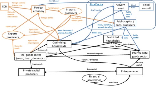
To better understand how the debt-to-GDP correction term affects the debt-to-GDP ratio stabilization for both fiscal rules, we simulate a deterministic increase in public consumption for two consecutive years, while having fiscal rules deactivated for three consecutive years. The increase of public consumption is such that it yields an increase of the debt-to-GDP ratio by about 30pp above its target at its peak. Then, fiscal rules ensure a gradual return of the debt-to-GDP ratio to its targeted level. Figure 2 depicts how the debt-to-GDP ratio responds to alternative strengths of the debt-to-GDP correction term in the fiscal rules.

Figure 2. Strength of the debt-to-GDP correction term and debt-to-GDP stabilization after a public consumption shock.

For clarity, we add a debt rule as the third fiscal rule, which contains only the debt correction term that is common to both rules. The results suggest that the behaviour of the debt-to-GDP ratio in case of the expenditure growth rule is more sensitive to the strength of the debt-to-GDP ratio correction term, compared to that of the structural balance rule, since the expenditure growth rule does not ensure debt-to-GDP ratio convergence without the debt correction term, while the structural balance rule does so. Also, the structural balance rule dampens the effect of the debt correction term on the debt-to-GDP ratio. For the benchmark calibration, the half-life of debt correction is similar across the two rules.

Looking at the deficit-to-GDP ratio behaviour (the middle panel of Figure 2), the debt rule imposes rapid fiscal tightening immediately after the fiscal rules are re-activated, while the expenditure growth rule postpones fiscal consolidation towards the future periods; the structural balance rule's behaviour fits in between these two cases. A slower fiscal consolidation yields faster GDP growth in the short term at the expense of slower economic growth in the future (the bottom panel of Figure 2).

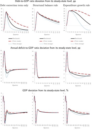
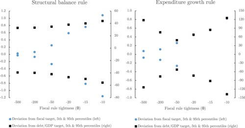
We set the persistence parameters ${\rho }_x$ to 0.5.²¹ As a benchmark, we prefer to assume the government meets the fiscal rules diligently, so that any differences in outcomes would be accounted for solely by the differences in the rules, and not by differences in how the government is following them. Therefore, we impose relatively tight fiscal rules. In order to calibrate their values, we simulate the model on a grid of their values for 10 thousand quarters and observe the amplitudes of the deviations of the fiscal outcomes from their targets (the term inside the large parenthesis in the fiscal rules) as well as the deviations of the debt-to-GDP ratio from its target.

We then set the fiscal tightness parameter such that the deviation from the fiscal target is within 0.3pp in 90% of time (which yields $\theta =-50$, see Figure 3). The simulated deviation of the debt-to-GDP ratio from its target is not very sensitive to the calibrated tightness parameter for the structural balance rule.²² However, for the expenditure growth rule the debt-to-GDP ratio volatility shows a non-linear pattern, first shrinking with the tightening of the fiscal rule then increasing (in our case, starting at about $\theta =-50$).²³ We contemplate that the government would not choose an extremely tight expenditure growth rule that would actually make its debt-to-GDP ratio volatility worse, thus we consider that setting $\theta =-50$ in our model is about optimal for stabilizing the debt-to-GDP ratio in the case of the expenditure growth rule.

Figure 3. Calibration of the fiscal rule tightness parameter.

Having selected relatively tight fiscal rules, we now proceed by inspecting how the structural balance and expenditure growth rules differ in stabilizing macroeconomic and fiscal variables.²⁴

6.2. Volatility analysis

We stochastically simulate the first-order approximation of the model by drawing from the estimated shock distributions.²⁵ We are fixing the random number generator's seed so that our simulation results are replicable and comparable across alternative rules. We are simulating the model economy for a sufficiently long period (10 thousand quarters) so that the statistics are relatively stable, as public debt cycles in our simulations can spread over many decades.

First, we visually compare government deficit with regard to the two rules. Figure 4 depicts simulated deficit and structural deficit, both in terms of per cent shares in GDP, for the two rules. For visibility purposes we constrain the plotted sample for the first 1000 quarters.

Figure 4. Comparison of deficit behaviour for the two fiscal rules.

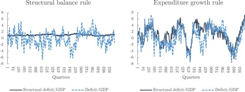
Inspecting Figure 4 demonstrates that the two rules yield different deficit behaviour. The structural balance rule ensures that the structural deficit is stable around the target (in our case, 0.9% of GDP), with minor deviations coming mainly from the correction for debt deviations. Meanwhile, the structural balance is drifting in a relatively wide interval for the expenditure growth rule, as this rule does not target the stability of the structural balance. Also, deficit volatility is visibly larger in the case of the expenditure growth rule.

Figures 3 and 4 indicate that the expenditure growth rule yields more volatile public finances, compared to the structural balance rule. This result could have been expected, as the expenditure growth rule is designed with a focus of stable public expenditure growth (apart from the term for the debt-to-GDP ratio correction which leads to adjustments in the medium term). Therefore, over the business cycle stable public expenditure growth results in more volatile public finances relative to GDP. Next, we will inspect how well the expenditure growth rule performs in terms of stabilizing the economy as well as the role of key modifications of the public expenditure definition entering the expenditure growth rule.

Table 1 reports volatility measures for several simulated public finance and macroeconomic series under the expenditure growth rule relative to the structural balance rule.²⁶ That is, a number above unity means higher volatility of a particular variable in case of the expenditure growth rule relative to the structural balance rule, and vice versa. Standard deviation is reported for all the listed variables. In addition, to better reflect a measure of the debt sustainability, the relative 95th percentile is reported additionally for the deviation of the debt-to-GDP ratio from its target. Its value above unity means that there are more extreme deviations of debt-to-GDP ratio from its target under the expenditure growth rule, compared to the structural balance rule.²⁷ Column 1 of Table 1 demonstrates that the volatility of public finances is larger in the case of the expenditure growth rule, compared to the structural balance rule, while the volatility of macroeconomic variables tends to be lower. In order to understand the differences, we will study the role of expenditure modification in the expenditure growth rule in what follows.

Table 1. Volatility measures for public finances and macroeconomic quantities under the expenditure growth rule relative to the structural balance rule.

Notes: Each number is a relative volatility measure of a particular variable for the expenditure growth rule, compared to the structural balance rule. A number below unity means the volatility of a series is smaller for the expenditure growth rule, and vice versa. The quantities GDP, consumption, and investment are reported in annual growth terms and inflation in annual terms.

6.2.1. Role of cyclical unemployment benefits

For understanding the differences between the expenditure growth and structural balance rules, we start by undoing some of the modifications of public expenditure that enters the expenditure growth rule. As a first step, we add cyclical unemployment benefits back to modified expenditure:

The results are reported in column 2 of Table 1. Comparing the results of the original expenditure growth rule with those of column 2 demonstrates that removing cyclical unemployment benefits from the public expenditure does not increase public debt volatility but (slightly) stabilizes macroeconomic volatility, as the public expenditure becomes less procyclical. Thus, our results support the choice of removing cyclical unemployment benefits from public expenditure.

6.2.2. Role of interest payments

Next, to examine the effect of the exclusion of debt service payments, we add interest payments back to the modified expenditure of the original expenditure growth rule:

The resulting volatility is reported in column 3 of Table 1. Comparing column 3 (interest payments included) to column 1 (the original rule) we can see that having interest payments in the modified expenditure reduces public debt volatility considerably, as now changes in debt service payments are taken into account by the fiscal rule. Also, the effect of having debt service payments in the expenditure growth rule increases the macroeconomic volatility only slightly, hence having more balance between the stability of public finances and the stability of macroeconomic variables. These results suggest that the choice of excluding the entire interest payments from the expenditure growth rule cannot be unequivocally supported; that is, there is evidence of only a marginal benefit in terms of macroeconomic stabilization in a monetary union context, while we see a relatively more pronounced deterioration of public finance volatility.

6.2.3. Constant interest rate in the expenditure growth rule

Interest payments are excluded from the expenditure growth rule based on the considerations that governments cannot fully control them. Therefore, governments should not be penalized for any ex post interest payments deviation from their ex ante estimate. In order to isolate the effect of changes in the interest rate (which the government cannot fully control) from changes in public debt, we consider including interest payments in the expenditure growth rule with a fixed interest rate. In the model, we set it to its steady state value:

while, in practice, the governments could use the projected long-run level. Column 5 of Table 1 demonstrates that having a constant interest rate in modified expenditure reduces public finance volatility, relative to the benchmark expenditure growth rule. Therefore, accounting at least for some part of debt service payments (the debt part) may help stabilize public finances. Another option for stabilizing public finances is raising debt correction strength, as is shown in the Online Appendix.

6.2.4. Total effect of expenditure modification

In order to assess the total effect of expenditure modification, we enter non-modified government expenditure in the expenditure growth rule. Essentially, the total effect is a sum of the effects from having cyclical unemployment benefits, interest payments, and averaging investment. The results are reported in column 4 of Table 1. Without any expenditure modification and for a comparable public finance volatility (which is subject to the choice of debt correction strength), the relative volatility of macroeconomic variables for the expenditure growth rule tends to be lower than that for the structural balance rule.

6.2.5. Role of government risk premium

In the model, there are both exogenous shocks to government risk and the endogenous risk premium due to deviations of public debt from its target. During the estimation sample, in particular during the 2009 bust period, the government risk premium shocks were sizeable. Also, due to debt deviations from its target, the endogenous risk premium affects the size of interest payments in simulations and thus further amplifies volatility of public debt. In order to control for the effect of the government risk premium channel, we shut off all exogenous shocks to the government risk premium as well as remove the endogenous government risk premium channel. In this case, changes in the government bond yield are solely due to changes in the ECB policy rate, which till recently has fluctuated in a relatively narrow interval. We redo simulations for both the expenditure growth and structural balance rule and report the results in column 6 of Table 1. As expected, nullifying the government risk premium reduces the public finance volatility in case of the expenditure growth rule relatively more than in case of the structural balance rule.

6.2.6. Stability of public investment

Much of the discussion on fiscal rules in the EU involves considerations of the stability of public investment, as it is seen as a contributing factor to long-run growth. It is also argued that, during recessions and in order to meet their fiscal constraints, governments are prone to cut, first and foremost, public investment. Our comparison of the structural balance and the expenditure growth rules in stochastic simulations (in Table 1) demonstrates that public investment is more stable under the expenditure growth rule, compared to the structural balance rule. This is because the expenditure growth rule (i) ignores the short-term economic fluctuations by targeting long-run growth, (ii) excludes interest payments from the modified expenditure definition, and (iii) uses a four-year average public investment in the modified expenditure definition.²⁸ Thus, the expenditure growth rule is more favourable to the stability of public investment, in line with economic reasoning.

6.2.7. Welfare implications

For welfare comparison we perform stochastic simulations to the second-order approximation with pruning in Dynare for 4000 quarters with a burn-in period of 500 quarters to give the model sufficient time to converge to the new stochastic steady state before using the simulated data (i.e. the remaining 3500 quarters) in the computation of moments needed for the welfare analysis. We consider two welfare measures. The first one is the standard measure in DSGE models where the welfare gain or loss is defined in consumption equivalent units. The second one defines the welfare gain or loss in terms of a percentage difference, since the former measure is sensitive to the calibration of the time discount factor β. We define our measure of welfare for the two types of households largely following Ascari et al. (2018) and Tsiaras (2020). The details are relegated to the Online Appendix.

In Table 1 we have documented that private consumption volatility is lower under the expenditure growth rule, compared to the structural balance rule. Since households dislike consumption volatility, the expenditure growth rule yields higher household welfare, especially for the restricted households. The aggregate household welfare gain from having the expenditure growth rule is 4% (0.7% in lifetime consumption equivalent units).

7. Sovereign monetary policy case

In order to assess whether endogenous monetary policy brings about any differences in our results, we now consider the case in which our model economy has its own currency and monetary policy characterized by inflation targeting. Therefore, we endogenize the nominal exchange rate, add the Fisher equation, as well as introduce a standard Taylor rule for the monetary authority: (9) $\ln \left(\frac{R_t}{R}\right)={\rho }_r\ln \left(\frac{R_{t-1}}{R}\right)+(1-{\rho }_r)(r_{\pi }\ln \left(\frac{{\pi }_t^{c,\mathrm{yoy}}}{{\pi }^{c,\mathrm{yoy}}}\right)+r_y\ln \left(\frac{y_t}{y}\right))+{ϵ}_{R_t},$(9) where ${\pi }_t^{c,\mathrm{yoy}}$ is the annual inflation rate, the persistence parameter ${\rho }_r$ is set to 0.8, the parameter controlling the reaction to CPI inflation deviation from its target $r_{\pi }$ is set to 1.5, and the reaction to the output gap is controlled by $r_y=0.125$.

Also, for symmetry, we replace the government bond yield specification with the one where the government bond yield is linked to the domestic monetary policy rate $R_{g,t}={\mathrm{\Phi }}_{g,t}{R}_t$, with the sovereign risk premium being affected by the public debt deviation from its target, (10) ${\mathrm{\Phi }}_{g,t}={\tilde{\varphi }}_{g,r}(\frac{D_{g,t}}{Y_t+Y_{t-1}+Y_{t-2}+Y_{t-3}}-\overline{\mathrm{dgy}})+{ϵ}_{g,t}^{\mathrm{rp}}.$(10) Then, we repeat the comparison of fiscal rules in terms of their implied fiscal and macroeconomic volatility, as reported in Table 2.

Table 2. Volatility measures for public finances and macroeconomic quantities under the expenditure growth rule relative to the structural balance rule – sovereign monetary policy case

Notes: Each number is a relative volatility measure of a particular variable for the expenditure growth rule, compared to the structural balance rule. A number below unity means the volatility of a series is smaller for the expenditure growth rule, and vice versa. The quantities GDP, consumption, and investment are reported in annual growth terms and inflation in annual terms.

First, we see that the results broadly hold for a sovereign monetary policy, that is, the expenditure growth rule stabilizes macroeconomic quantities relatively more, but public finances relatively less. For the benchmark specifications, the effects with a sovereign monetary policy are even more pronounced, as visible in Table 2, first column.

Second, when including the interest payments back to the expenditure growth rule, the volatility of public finances falls, as seen in the monetary union case. However, distinctively, also the relative ability of the expenditure growth rule to stabilize macroeconomic volatility decreases considerably (Table 2, third column). This result turns out to be robust for alternative specifications of the Taylor rule, including the suspension of monetary policy shocks. Therefore, in a sovereign monetary policy environment, unlike a monetary union environment, the exclusion of interest payments helps stabilize macroeconomic variables. This result is linked to changes in the interest rate, as using a constant long-run interest rate in interest payments calculations re-establishes the benchmark results (Table 2, fifth column).

7.1. Monetary policy transmission channels

To understand the interest payments channel under an interest rate rule, we simulate a positive shock to the monetary policy rate. Figure 5 depicts comovement of the structural balance rule and monetary policy, while the fiscal response under the expenditure growth rule is muted.

Figure 5. Structural balance rule versus expenditure growth rule, sovereign monetary policy case – monetary policy shock.

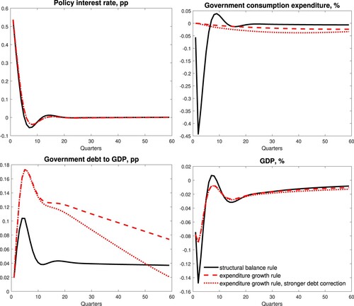
In practice, there are two main channels via which monetary policy affects fiscal positions. First, a higher policy rate raises public debt service payments, thus deteriorating the government budget balance (debt service payments channel). Second, monetary policy tightening weakens aggregate demand, thereby lowering the tax base and tax revenues, and ultimately worsening the government budget balance (revenue shortfall channel). The structural balance rule should, in principle, be unaffected by the revenue shortfall channel, as the structural balance corrects the budget balance for cyclical changes in the output gap. However, in practice, this correction may not fully capture shock-specific revenue elasticities, developments in profit-related taxes due to leads and lags in tax collection, consumption switching over the business cycle, structural changes in the economy, and other factors (see e.g. Morris et al., 2009). Moreover, the estimate of the structural balance rule is subject to measurement errors in the real-time estimate of the output gap. Therefore, fiscal policy would still be (somewhat) sensitive to the revenue windfall channel when the government faces a structural balance rule.

In our model, the revenue shortfall channel is muted, so the structural balance rule reacts to the debt service payments channel. Namely, whenever the structural balance deteriorates with respect to its target due to higher interest payments, the government cuts expenditure on other items. Thus, there is positive comovement between monetary and fiscal policies in the direction from monetary to fiscal policy under the structural balance rule. In contrast, the debt service payments channel is removed from the benchmark expenditure growth rule by removing debt service costs from the modified expenditure definition. Likewise, the expenditure growth rule is muted to the revenue windfall channel by construction in that the expenditure growth does not react to cyclical developments in tax revenues.

As a result, there is almost no endogenous fiscal response to a monetary policy shock under the expenditure growth rule. The deterioration in fiscal positions is thus reflected mostly in a higher government debt level. Note that the build-up of government debt is stronger under the expenditure growth rule than under the structural balance rule in the face of a monetary policy tightening shock. However, the convergence of government debt to its target under the expenditure growth rule can be facilitated by strengthening the role of the debt-correction term inherent in the expenditure growth rule.²⁹ More stable fiscal policy under the expenditure growth rule contributes to the stability of the economy over the business cycle frequency.

It appears a robust feature in our simulations³⁰ that accounting for interest payments in the fiscal rule may add to the volatility of the economy, although it helps stabilizing the trajectory of public debt. As the structural balance rule takes into account debt service payments but the benchmark expenditure growth rule does not, the debt service payments channel explains much of the superiority of the benchmark expenditure growth rule in stabilizing macroeconomic variables in a sovereign monetary policy regime.³¹

A note of caution, however, is that in our model, the government is assumed to only issue short-term government bonds. In reality, governments typically issue bonds with a longer maturity. In that case, the fiscal response to changes in the monetary policy stance under the structural balance rule would be more gradual than is predicted by the model.

7.2. Welfare implications

Similarly to the case of a small country in a monetary union, we do welfare computation also for a sovereign monetary policy case with the same methodology. The aggregate household welfare gain under the expenditure growth rule with sovereign monetary policy is slightly larger and equals 5% (1% in lifetime consumption equivalent units). The details are in Section 5 of the Online Appendix.

7.3. Fiscal dominance vs. monetary dominance

The recent prolonged period of historically low nominal interest rate and relatively large public debt levels has rekindled discussions about the fiscal theory of the price level (Leeper, 1991). According to this theory, when monetary policy is passive (i.e. it does not react strongly to inflation dynamics) and fiscal policy does not stabilize public debt a situation emerges that is called a fiscal dominance regime. Under this regime the price level would adjust to stabilize real outstanding government debt. It is contrary to a monetary dominance regime when monetary policy actively responds to inflation while fiscal policy adjusts public spending (and/or taxes) passively to stabilize the debt to GDP ratio.

In order to study a possible emergence of a fiscal dominance regime in our model we cut the inflation reaction parameter in the interest rate rule $r_{\pi }$ threefold to 0.5 (from the original value of 1.5) as in Hinterlang and Hollmayr (2022), and reduce the tightness of our fiscal rules tenfold, i.e. we set ${\varphi }_{x,\mathrm{sdy}}={\varphi }_{x,\mathrm{ggap}}=-5$ from the original values of $-50$. Note that we are not able to shut down the fiscal rules entirely, as it is incompatible with the model stability. It is an expected behaviour, as our model features several open economy dimensions that weaken the domestic price adjustment.

As a result, although inflation being more than twice as volatile with passive monetary policy, the price adjustment is not enough to stabilize the public debt. Therefore, weak fiscal rules amplify the government debt-to-GDP fluctuations under both fiscal rules. However, given the evidence shown in Figure 3 that the debt volatility under the expenditure growth rule is much more sensitive to the calibration of the fiscal rule tightness parameter compared to the structural balance rule, a much weaker expenditure growth rule amplifies the public debt volatility multiple times stronger than a much weaker structural balance rule (see Table 6.1 in the Online Appendix). This simulation exercise emphasizes once again the crucial role of a proper calibration of the debt correction term in the expenditure growth rule in practice that would be strong enough to ensure the public debt convergence to its target in a timely manner.

8. Conclusion

There has been a discussion about the European Union's fiscal framework with the aim of simplifying it. Although the new fiscal framework that is on the horizon may not turn out to be considerably simpler, it in accordance with the previous discussion it tends to be more flexible and put more weight on the expenditure fiscal rule. Our paper quantitatively compares two benchmark operational fiscal rules that have been discussed in several fora, and are used by the European Commission – the structural balance rule and the expenditure growth rule. The main innovation of this paper is the detail in which we consider the fiscal rules and that we use both stochastic and deterministic simulations of a small open economy DSGE model with a rich fiscal sector to quantitatively evaluate each fiscal rule's performance, including the analysis of expenditure modifications. As such, our study helps understanding the trade-offs and quantitative differences between the alternative fiscal rules. We consider both the case of a small open economy in a monetary union and the case of a small open economy with sovereign monetary policy to study a monetary-fiscal interaction.

The main finding of our study is that the expenditure growth rule tends to yield somewhat more stable macroeconomic outcomes than the structural balance rule at the cost of causing more volatile public debt. The main channel for the discrepancy between the expenditure growth targeting and the public debt-to-GDP ratio stabilization objective is the removal of interest payments from public expenditure in the modified public expenditure definition used in the expenditure growth rule.

Moreover, the expenditure growth rule is more sensitive to the strength of the public debt-to-GDP ratio correction term than the structural balance rule as it is unable to stabilize debt without such a debt anchor. Therefore, more importance to a sufficiently strong debt correction term is advised under the expenditure growth rule to contain public debt volatility, compared to the structural balance rule.

In terms of the timing of fiscal adjustments after a fiscal expansion, the expenditure growth rule tends to postpone fiscal consolidation to future periods, as compared to the structural balance rule, implying that the resulting growth outcomes under the expenditure growth rule are larger in the short run but smaller in the future.

Accounting for interest payments in fiscal rules amplifies the co-movement between monetary and fiscal policies. The reason is that monetary policy stance affects the government debt service payments. Our simulation results, however, reveal that accounting for interest payments in fiscal rules may be detrimental to macroeconomic stability over the business cycle.

The welfare of households is higher with an active expenditure growth rule than with an active structural balance rule. This holds both for a country in a monetary union and for a country with sovereign monetary policy. However, the welfare gain would be lower if the interest payments were taken into account in the expenditure growth rule.

In the Online Appendix, besides various robustness and sensitivity analyzes, we also consider a variant of our benchmark fiscal rules termed the golden rule that excludes public investment from fiscal rules. This helps safeguarding public investment and leads to higher growth outcomes during a period of a considerable and persistent boost in public investment (e.g. the Next Generation EU programme).

Overall, our results indicate that the expenditure growth rule with a sufficiently strong debt correction term may strike the right balance between the short-term economic stabilization and medium-term public debt convergence objectives.

Acknowledgments

We would like to thank anonymous referees, António Afonso, Kea Baret (discussant), the seminar participants at Latvijas Banka, Lietuvos Bankas, the European Commission, the Ministry of Finance of Latvia, the Fiscal Discipline Council of Latvia, the Baltic Central Bank Research Meeting 2021, and the conference participants at the 20th Journées Louis-André Gérard-Varet, the 9th UECE Conference on Economic and Financial Adjustments, the 4th ERMEES Macroeconomics Workshop, the Scottish Economic Society 2022 Annual Conference, the 28th International Conference on Computing in Economics and Finance (CEF 2022), and the 2022 Dynare Conference for their helpful comments and constructive suggestions. The views expressed herein are solely those of the authors and do not necessarily reflect the views of Latvijas Banka or the Eurosystem.

Disclosure statement

No potential conflict of interest was reported by the author(s).

Additional information

Notes on contributors

Ginters Bušs

Ginters Bušs holds a Doctor of Engineering (Dr.sc.ing.) degree in Information Technology from Riga Technical University, a Master of Social Sciences degree in Law with distinction from the University of Latvia and a Master of Economics degree from Central European University in Hungary. He has studied economics also at Duke University in the USA and Ghent University in Belgium. He joined Latvijas Banka in 2011 as a Senior Econometrician in the Monetary Research and Forecasting Division of the Monetary Policy Department, later as Principal Econometrician. Ginters is the author of the Latvian DSGE model, many scientific studies, articles and Macroeconomic Developments Report scenarios. He has also developed the GDP forecasting system at Latvijas Banka and previously - the Central Statistical Bureau of Latvia. He represents Latvijas Banka in the Working Group on Econometric Modelling of the European System of Central Banks.

Patrick Grüning

Patrick Grüning holds a PhD from Goethe University Frankfurt in business administration (2015) and a “Diplom” degree in mathematics (2009). His doctoral dissertation was prepared within the Ph.D. in Finance program at the Graduate School of Economics, Finance, and Management of Goethe University Frankfurt and carries the title “Essays on Asset Pricing with Contagion, Endogenous Growth, and Long-run Risk”. During his studies he visited the Sauder School of Business at the University of British Columbia for 6 months (2011/2012) and spent a semester at the University of Wisconsin-Superior (2006).Patrick Grüning joined the Monetary Policy Department of the Bank of Latvia in October 2021. Before his employment at the Bank of Latvia he worked at the Bank of Lithuania from September 2015 to June 2021 and at the Research Center SAFE of Goethe University Frankfurt (now the Leibniz Institute for Financial Research SAFE) from March 2013 to August 2015. He is engaged in research on climate change economics, fiscal policy, macro-finance, and asset pricing.

Oļegs Tkačevs

Oļegs Tkačevs is a Principal Economist at the Bank of Latvia. His main research activities include fiscal and structural policies, competitiveness and trade. In the past he represented the Bank of Latvia in the ESCB Working Group of Public Finance. During the great recession period he closely cooperated with counterparts from the IMF and EC on fiscal consolidation strategy and recommendations for structural reforms. In 2012 and 2013, he was an NCB expert at the Directorate General Economics of the European Central Bank. He holds a Ph.D. in Economics from the University of Latvia.

Notes

1 Article 126 and Protocol annexed to the TEU.

2 Council Regulation 1467/97.

3 Council Regulation 1466/97.

4 Council Regulation 1055/2005.

5 The Treaty on Stability, Coordination and Governance in the Economic and Monetary Union, signed by all EU countries except Czechia and the UK.

6 Regulation (EU) 1173/2011.

7 Council Directive 2011/85/EU.

8 Regulation (EU) 1177/2011.

9 It is now required that a member state with a debt-to-GDP ratio above 60% reduces the gap to this level annually by 5%.

10 Regulation (EU) 1175/2011.

11 Alternatively, Blanchard et al. (2021) suggest abandoning fiscal rules in favour of country-specific standards.

12 Christofzik et al. (2018) consider annual debt-to-GDP corrections of 1.33% (1/75) and 2% (1/50).

13 In particular, when the excessive deficit procedure is opened on the basis of the deficit criterion, the corrective net expenditure path should be consistent with a minimum annual structural adjustment of at least 0.5% of the GDP. The annual minimum adjustment steps of 0.5% of GDP may exclude interest payments until year 2027.

14 The legislative package consists of three documents: a regulation on the preventive arm https://www.consilium.europa.eu/media/70386/st06645-re01-en24.pdf a directive https://data.consilium.europa.eu/doc/document/ST-15396-2023-REV-4/en/pdf and a regulation on the corrective arm https://data.consilium.europa.eu/doc/document/ST-15876-2023-REV-4/en/pdf.

15 Additionally, there is wasteful spending, which is constant and exogenous, and has the role of a residual in the steady state.

16 They need to pay quadratic adjustment costs for holdings in excess of an amount they can hold for free.

17 However, we keep reporting the annual balance-to-GDP ratio in the tables below for the reader's convenience.

18 The alternative measures we considered were: the employment gap ${\mathrm{ygap}}_t=\ln \left(L_t/L\right)$, where $L_t$ is total labour supply and L its value in the deterministic steady state, a measure based on capital and labour utilization rates ${\mathrm{ygap}}_t=\ln \left[{\left(\frac{u_t}{u}\right)}^{\alpha }{\left(\frac{L_t}{L}\right)}^{1-\alpha }\right]$and their time-varying equilibria specifications where $u_t$ and u is the capital utilization rate at time t and the steady-state capital utilization rate, respectively. However, we found that our benchmark specification matches the data the best, since the capital utilization rate is trending in our data sample. Section 7.2 of the Online Appendix compares empirical estimates of the output gap with those generated with our DSGE model in pseudo real time. Our benchmark output gap measure is a popular one used in practice (also in simpler semi-structural models). An alternative approach in DSGE models is also to use the level of output relative to the flexible price output level as the output gap; however, this is more difficult to use in practice, especially given the size of our model, and since our paper tries to answer the research question from an applied perspective, we keep our simple proxy of the output gap.

19 Note that the debt-correction term depends on the deviation of the annual debt-to-GDP ratio from its target for simplicity. Moreover, we have also experimented with using three-year averages of the debt-to-GDP ratio in these fiscal rules. The results reported below remain basically unaltered. See also Footnote ²² as well as Figure 6.4 and Table 6.1 in the Online Appendix.

20 For the expenditure growth rule, our benchmark calibration implies ${\varphi }_{x,d}=\left(1/100\right)/(4\cdot 0.38)$ where 4 is used to convert to the quarterly expenditure growth rule and 0.38 is our calibrated government expenditure share in GDP.

21 We have not found much sensitivity of our key results to the calibration of this persistence parameter.

22 About up to a 40pp deviation across all calibrations.

23 This non-linear behaviour is robust to an alternative fiscal rule specification with a 3-year average debt-to-GDP targeting (as practised by the European Commission), instead of targeting the particular period's debt-to-GDP deviation; see Figure 6.4 in the Online Appendix. A minor twist in the behaviour is the need for a stronger debt correction with a longer averaging window.

24 Note that in the model and thus also in the results discussed below we always have three fiscal rules active: one for public consumption expenditure, one for public investment expenditure, and one for government transfers. One might suspect that the results can be different if only one of these rules is active at a time. In particular, it might be argued that public investment expenditure should not be touched in order not to harm future growth prospects. Similarly, the amount of government transfers cannot be easily or quickly changed, when a government faces political or economic pressure to reduce total government spending, so that it could only adjust government consumption expenditure effectively. However, it turns out, using unreported results available from the authors upon request, the outcomes we are going to discuss below are qualitatively robust and quantitatively not much different from the number and kind of fiscal rules active in the model (we do not consider public investment as a single rule, as it is unlikely in policy practice). One just has to adjust the fiscal rule parameters (by making them larger in absolute value) in order to keep the volatility of the public debt-to-GDP ratio unchanged, relative to the benchmark calibration with all three fiscal rules.

25 Relative to the estimated shocks, we are downscaling all the estimated shock standard deviations by 20% (or variance by 36%), as the shocks are estimated to Latvian data and Latvia experienced an exceptionally large boom-bust cycle in the first decade of this century so that the simulation results would be more tailored to the post-2009 recession period (and to more stable economies).

26 As a robustness check, Table 6.1 in the Online Appendix reports the results for the alternative specification of fiscal rules, where the government is targeting a 3-year average debt-to-GDP deviation from its target, instead of the particular period's debt-to-GDP targeting. The results are similar.

27 Also, given a roughly symmetric distribution of debt-to-GDP from its target (observed in Figure 3), this measure shows roughly how many times a 90% interval of debt-to-GDP ratio deviations (in both positive and negative direction) from its target is wider under the expenditure growth rule, compared to the structural balance rule.

28 Public investment averaging yields small improvements in public investment stability in stochastic simulations for typical public investment shocks. We return to this topic during the discussion of the golden rule below.

29 In the simulation with faster debt convergence, the debt-correction term is made twice stronger. Absent the expenditure growth targeting, this would imply speeding up the rate of annual debt-to-GDP gap correction from 1/25 to 2/25. Yet, the presence of the expenditure growth target alters the actual rate of debt convergence in a non-linear way.

30 We have experimented with both alternative Taylor rule specifications and alternative macroeconomic shocks, including their assumed persistence parameters.

31 We confirm this result also by excluding interest payments from the structural balance rule and verifying that in this case much of the superiority of the expenditure growth rule in stabilizing macroeconomic outcomes disappears.

References

- Adolfson, M., Laséen, S., Lindé, J., & Villani, M. (2008). Evaluating an estimated new Keynesian small open economy model. Journal of Economic Dynamics and Control, 32(8), 2690–2721. https://doi.org/10.1016/j.jedc.2007.09.012
- Andrle, M., Bluedorn, J. C., Eyraud, L., Kinda, T., Brooks, P. K., Schwartz, G., & Weber, A. (2015). Reforming fiscal governance in the European union (IMF Staff Discussion Notes 15/9). International Monetary Fund.
- Ascari, G., Phaneuf, L., & Sims, E. (2018). On the welfare and cyclical implications of moderate trend inflation. Journal of Monetary Economics, 99, 56–71. https://doi.org/10.1016/j.jmoneco.2018.06.001
- Bayoumi, T., Goldstein, M., & Woglom, G. (1995). Do credit markets discipline sovereign borrowers? Evidence from the U.S. States. Journal of Money, Credit and Banking, 27(4), 1046–1059. https://doi.org/10.2307/2077788
- Benassy-Quere, A., Brunnermeier, M., Enderlein, H., Farhi, E., Fratzscher, M., Fuest, C., Gourinchas, P.-O., Martin, P., Pisani-Ferry, J., Rey, H., Schnabel, I., Veron, N., di Mauro, B. W., & Zettelmeyer, J. (2018). Reconciling risk sharing with market discipline: A constructive approach to euro area reform (CEPR Policy Insight 91).
- Bernanke, B., Gertler, M., & Gilchrist, S. (1999). The financial accelerator in a quantitative business cycle framework. In J. B. Taylor & M. Woodford (Eds.), Handbook of macroeconomics (Vol. 1, 21, pp. 1341–1393). Elsevier Science.
- Blanchard, O., Leandro, A., & Zettelmeyer, J. (2021). Redesigning EU fiscal rules: From rules to standards. Economic Policy, 36(106), 195–236. https://doi.org/10.1093/epolic/eiab003
- Bruck, T., & Zwiener, R. (2006). Fiscal policy rules for stabilisation and growth: A simulation analysis of deficit and expenditure targets in a monetary union. Journal of Policy Modeling, 28(4), 357–369. https://doi.org/10.1016/j.jpolmod.2006.01.004
- Bundesbank (2019). Reforming the stability and growth pact: Striving for sustainability while offering room for manoeuvre (SUERF Policy Note, No. 111).
- Bušs, G. (2017). Wage formation, unemployment and business cycle in Latvia (Latvijas Banka Working Paper No. 1/2017).
- Bušs, G., & Grüning, P. (2023). Fiscal DSGE model for Latvia. Baltic Journal of Economics, 23(1), 1–44. https://doi.org/10.1080/1406099X.2023.2173915
- Carnot, N. (2014). Evaluating fiscal policy: A rule of thumb (European Economy – Economic Papers 2008–2015 526). Directorate General Economic and Financial Affairs (DG ECFIN), European Commission.
- Christiano, L. J., Eichenbaum, M. S., & Evans, C. L. (2005). Nominal rigidities and the dynamic effects of a shock to monetary policy. Journal of Political Economy, 113(1), 1–45. https://doi.org/10.1086/426038
- Christiano, L. J., M. S. Eichenbaum, & Trabandt, M. (2016). Unemployment and business cycles. Econometrica, 84(4), 1523–1569. https://doi.org/10.3982/ECTA11776
- Christiano, L. J., Trabandt, M., & Walentin, K. (2021). Involuntary unemployment and the business cycle. Review of Economic Dynamics, 39, 26–54. https://doi.org/10.1016/j.red.2020.05.003
- Christofzik, D., Feld, L., Reuter, W. H., & Yeter, M. (2018). Uniting European fiscal rules: How to strenghten the fiscal framework (Working Papers 04/2018). German Council of Economic Experts/Sachverständigenrat zur Begutachtung der gesamtwirtschaftlichen Entwicklung.
- Claeys, G., Darvas, Z., & Leandro, A. (2016). A proposal to revive the European fiscal framework (Policy Contribution 2016/07). Bruegel.
- Coibion, O., Gorodnichenko, Y., & Ulate, M. (2018). The cyclical sensitivity in estimates of potential output. Brookings Papers on Economic Activity, 28(4), 343–411. https://doi.org/10.1353/eca.2018.0020
- Cordes, T., Kinda, T., Muthoora, P. S., & Weber, A. (2015). Expenditure rules; effective tools for sound fiscal policy? (IMF Working Papers 15/29). International Monetary Fund.
- Darvas, Z., Martin, P., & Ragot, X. (2018). European fiscal rules require a major overhaul (Bruegel Policy Contribution No. 2018/18).
- Debrun, X., & Jonung, L. (2019). Under threat: Rules-based fiscal policy and how to preserve it. European Journal of Political Economy, 57(C), 142–157. https://doi.org/10.1016/j.ejpoleco.2018.09.001
- Debrun, X., Moulin, L., Turrini, A., Kumar, M. S., Drazen, A., & Fuest, C. (2008). Tied to the mast? National fiscal rules in the European Union [with discussion]. Economic Policy, 23(54), 297–362. https://doi.org/10.1111/j.1468-0327.2008.00199.x
- European Commission (2019). Vade Mecum on the stability & growth pact, 2019 Edition (Institutional Paper 101).
- European Fiscal Board (2019). Assessment of EU fiscal rules with a focus on the six and two-pack legislation.
- Eyraud, L., Debrun, X., Hodge, A., Lledo, V. D., & Pattillo, C. A. (2018). Second-generation fiscal rules; balancing simplicity, flexibility, and enforceability (IMF Staff Discussion Notes 18/04). International Monetary Fund.
- Fatas, A., & Mihov, I. (2003). The case for restricting fiscal policy discretion. The Quarterly Journal of Economics, 118(4), 1419–1447. https://doi.org/10.1162/003355303322552838
- German Council of Economic Experts (2017). Towards a forward-looking economic policy (Annual Report).
- Hall, R. (2005a). Employment efficiency and sticky wages: Evidence from flows in the labor market. Review of Economics and Statistics, 87(3), 397–407. https://doi.org/10.1162/0034653054638346
- Hall, R. (2005b). Employment fluctuations with equilibrium wage stickiness. American Economic Review, 95(1), 50–65. https://doi.org/10.1257/0002828053828482
- Heinemann, F., Moessinger, M.-D., & Yeter, M. (2018). Do fiscal rules constrain fiscal policy? A meta-regression-analysis. European Journal of Political Economy, 51, 69–92. https://doi.org/10.1016/j.ejpoleco.2017.03.008
- Hinterlang, N., & Hollmayr, J. (2022). Classification of monetary and fiscal dominance regimes using machine learning techniques. Journal of Macroeconomics, 74, 103469. https://doi.org/10.1016/j.jmacro.2022.103469
- International Monetary Fund (2014). Public expenditure reform: Making difficult choices (Fiscal Monitor).
- Kamps, C., & Leiner-Killinger, N. (2019). Taking stock of the functioning of the EU fiscal rules and options for reform (Occasional Paper Series 231). European Central Bank.
- Kamps, C., Leiner-Killinger, R. D. S. N., Ruffer, R., & Sondermann, D. (2014). The identification of fiscal and macroeconomic imbalances – unexploited synergies under the strengthened EU governance framework (Occasional Paper Series 157). European Central Bank.
- Kinda, T. (2015). Anchoring sustainable fiscal policy: A new fiscal rule in Canada (Selected Issues Paper, IMF Country Report 15/23). International Monetary Fund, Washington.
- Laxton, D., Mursula, S., Kumhof, M., & Muir, D. V. (2010). The global integrated monetary and fiscal model (GIMF)–theoretical structure (IMF Working Papers, 2010 (034)).
- Leeper, E. M. (1991). Equilibria under ‘active’ and ‘passive’ monetary and fiscal policies. Journal of Monetary Economics, 27(1), 129–147. https://doi.org/10.1016/0304-3932(91)90007-B
- Levin, J. (1983). A model of stabilization policy in a jointly floating currency area. In J. Bhandari & B. Putnam (Eds.), Economic interdependence and flexible exchange rates (pp. 329–349). MIT Press.
- Ljungman, G. (2008). Expenditure ceilings—a survey (IMF Working Papers 08/282). International Monetary Fund.
- Morris, R., Braz, C. R., de Castro, F., Jonk, S., Kremer, J., Linehan, S., Marino, M. R., Schalck, C., & Tkacevs, O. (2009). Explaining government revenue windfalls and shortfalls: An analysis for selected EU countries (European Central Bank Working Paper No. 1114).
- Mortensen, D. T., & Pissarides, C. A. (1994). Job creation and job destruction in the theory of unemployment. The Review of Economic Studies, 61(3), 397–415. https://doi.org/10.2307/2297896
- Schmitt-Grohé, S., & Uribe, M. (2012). What's news in business cycles. Econometrica, 80(6), 2733–2764. https://doi.org/10.3982/ECTA8050
- Shimer, R. (2005). The cyclical behavior of equilibrium unemployment and vacancies. American Economic Review, 95(1), 25–49. https://doi.org/10.1257/0002828053828572
- Shimer, R. (2012). Reassessing the ins and outs of unemployment. Review of Economic Dynamics, 15(2), 127–148. https://doi.org/10.1016/j.red.2012.02.001
- Symansky, S. A., Debrun, X., & Epstein, N. P. (2008). A new fiscal rule; should Israel “Go Swiss” (IMF Working Papers 08/87). International Monetary Fund.
- Tsiaras, S. (2020). Financial crisis, monetary Base expansion and risk (Unpublished Working Paper).
- Wyplosz, C. (2012). Fiscal rules: Theoretical issues and historical experiences. In Fiscal policy after the financial crisis (pp. 495–525). NBER Chapters, National Bureau of Economic Research, Inc.