Predicting the impacts of clearing on vegetation communities: a model-based approach for identifying conservation priorities in Queensland, Australia

ABSTRACT

Predicting outcomes is critical for conservation prioritisation. We predicted the areas that are likely to be impacted using a generalised estimating equation from a logistic regression and intersected our model with vegetation community mapping for Queensland, Australia. Under the assumption that areas with a high probability of clearing would eventually be cleared, we identified vegetation communities at risk of transitioning into a more vulnerable status, addressing a critical knowledge gap. Specifically, we identify: 1) areas within the study region's bioregions face the highest risk of forest cover loss; 2) communities may transition to more vulnerable according to their extent-based vulnerability status. Our analysis determined high-risk areas within the study region and vegetation communities vulnerable to changing status. Three clearing scenarios – low, moderate and high – were evaluated. In the low scenario, 0.3 per cent of vegetation communities experienced clearing, with 26 communities changing their status. The moderate scenario impacted 35 per cent of vegetation communities, with 103 communities at risk. In the high scenario (our most aggressive assumption), 45 per cent of vegetation communities overlapped with areas suitable for clearing, affecting the status of 158 communities. We emphaise the need to protect high-risk communities while implementing effective management strategies in areas where clearing poses minimal threat.

KEYWORDS:

• Habitat loss
• Queensland
• predictive modelling
• risk-based approach
• regional ecosystems
• vegetation

Introduction

Land clearing results from the interconnected dynamics of human populations and their economics, scientific and technological developments, cultural values and policies (Seabrook, McAlpine, and Fensham 2006; 2008). The consequences of land clearing for the environment include: reducing the extent and abundance of species (Haddad et al. 2015), habitat fragmentation (Holland and Bennett 2010) and decreased efficiency and functionality of ecological processes (Cogger et al. 2003). Due to the unprecedented expansion of built infrastructure and agriculture, approximately one quarter of all species from red-list assessed groups are classified as vulnerable to extinction (IPBES 2019), rendering habitat loss by land clearing a critical threatening process to biodiversity (Ceballos and Ehrlich 2002; Tilman et al. 2017). Accordingly, nations around the globe ratified the United Nations Convention on Biological Diversity in 1993, resulting in a cross-jurisdictional enterprise to slow habitat loss. Governments developed environmental programmes and policies to achieve this goal, including protected areas and environmental regulations.

Despite being considered a developed nation, Australia has globally high land-clearing rates (Evans et al., 2011; Carwardine et al., 2012). This threatening process is firmly attributed as the primary cause of biodiversity decline (Woinarski, Burbidge, and Harrison 2015). Most clearing of native vegetation has occurred on arable lands for agricultural and pastoral production (Evans 2016; McAlpine et al. 2009), with the majority of clearing occurring in the State of Queensland (Bradshaw 2012; Heagney, Falster, and Kovač 2021). For example, in the four years between 1991 and 1995, Queensland was responsible for 80 per cent of the 1.2 million ha cleared across Australia (Accad and Neldner 2015; Wilson, Neldner, and Accad 2002). Between 2001 and 2003, the total amount of woody vegetation in cleared in Queensland was 1.04 million ha (0.56 per cent of Queensland's total area) (Queensland Government 2018).

When Australia ratified the Convention on Biological Diversity, jurisdictional governments could access national funding in return for meeting national standards on vegetation cover. As a result, Queensland passed the Vegetation Management Act in 1999 (The Act) to address concerns over the effects of broad-scale clearing of native vegetation, encourage ecologically sustainable land use and maintain regional biodiversity. The primary intent of the Act is to avoid land degradation and maintain biodiversity and ecological processes. Following the prohibition of broad-scale clearing under the Act in 2006, clearing rates per year fell by over 200,000 ha between 2006 and 2010, marking a historic low for clearing rates in Queensland (Government 2015a; 2017). In 2013, however, the Act was amended, allowing for the resumption of broad-scale clearing for high-value dryland and irrigated agriculture as part of a government initiative to expand agricultural development. In the years that followed, Queensland's rate of land clearing soared to over 350,000 ha per year (Government 2015a). Recent statistics now show that Queensland's rate of land clearing is nearly 400,000 ha per year, making the state a global land-clearing hotspot (Hudson 2019). As a result of this extensive and ongoing clearing, many vegetation communities in Queensland are vulnerable to extinction (Tulloch et al. 2015).

Previous studies have commented on the substantial effects of rapid policy change on vegetation management in Queensland. For example, Taylor (2013) estimated that 1.3 million hectares of previously uncleared vegetation would be at risk of future clearing following the 2013 changes to the Act. In addition to the total extent of vegetation at risk, a 2017 study also found that the Act fails to protect the ecosystems experiencing the highest clearing rates (Rhodes et al. 2017). Similar to Taylor's findings, another recent study evaluated the impact of vegetation policy in Queensland and found that the Act was largely ineffective at curbing land clearing (Simmons et al. 2018). These studies demonstrate that existing policies have not had the desired impact of reducing land clearing and that the Act changes to make additional land available for future clearing. The risk of habitat loss and the associated consequences for wildlife is a function of both availability for clearing and the likelihood of clearing. Thus, it is also essential to determine the extent to which those areas not yet cleared and available for clearing under current vegetation management are likely to be cleared.

Strategic planning is critical to planning such programs by proactively identifying communities or ecosystems with the highest risk of loss. Without these forecasting, policies may be insufficient or ineffective in abating biodiversity loss. However, there is limited knowledge of the likelihood or probability of such loss across Australian landscapes. Such a critical knowledge gap fundamentally constricts decision-makers’ capacity to understand the effectiveness of a conservation action relative to inaction (Maron, Rhodes, and Gibbons 2013). Predicting clearing is thus crucial for informed decision-making in designing conservation interventions (Pressey et al. 2021).

Indeed, there is growing research interest in modelling change in land cover; specifically, the probability of natural habitat being converted to modified habitat (Wang et al. 2022). However, for these modelling approaches to be beneficial and integrated within an adaptive management framework, they must be easily accessible, allowing policymakers to rapidly produce and update policies in response to evolving human landscapes and drivers. In this study, our objectives were: 1) to identify areas where clearing is most likely to occur and 2) to identify previously uncleared vegetation communities most susceptible to changes in biodiversity status due to clearing pressure. To achieve this, we developed a predictive spatial model of clearing for the State of Queensland and intersected it with the state's vegetation community mapping. We present three scenarios of potential clearing: high, moderate and low and, for each scenario, tally the total area in each bioregion and the number of vegetation communities likely to be impacted by future clearing.

Methods

Study area

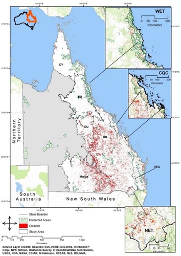
The study area constitutes nine of the thirteen bioregions in Queensland, Australia. Bioregions are areas with similar climate, geology and biota (Thackway and Cresswell 1997) and are Queensland's primary reporting unit for biodiversity conservation. We focused on the nine bioregions dominated by woody vegetation (Figure 1). We excluded four grassland-dominated bioregions (390,000 km² or 22.2 per cent of land area in the state) because such habitats are incompatible with the predictor variable of land clearing (described below). The bioregions in the study area are diverse and consist of extensive areas of savannah, a mosaic of mangroves, pastures and remnant tropical forests. Approximately 19 per cent of the land has been cleared (34,886,294 ha) since European colonisation (Queensland Department of Environment and Science 2018). Significant clearing drivers are urbanisation, cattle ranching, agricultural production and timber harvesting (Bradshaw 2012; Evans 2016; Seabrook, McAlpine, and Fensham 2006). Indeed, Queensland has experienced some of the world’s highest clearing rates for woody vegetation between 2015 and 2018 (Department of Science 1988-2016; Queensland Department of Environment and Science 2018), resulting in the classification of 45 per cent of regional ecosystems listed as ‘of concern’ or ‘endangered’ (n = 603, n = 96).

Figure 1. Map of the bioregions for this analysis. Areas that have been cleared in the last 30 years are shown in red (as defined by the Statewide Land and Trees Study (SLATS, Department of Science 1988-2016)). Protected areas as of 2019 are shown in green.

Data sources and pre-processing

Spatially explicit models of the probability of clearing can function as decision-support tools. However, care must be taken in their design because the factors influencing clearing vary globally and regionally (Simmons et al. 2018). Thus, the first modelling step is correctly identifying the proximate underlying and spatially explicit causes of clearing (the independent variables). We acknowledge that the decision to clear land is complex, driven by various factors, including personal and societal values and attitudes and legal and economic considerations. Although we recognise the importance of these variables, our study focused specifically on biophysical variables and the spatial extent to which possible land clearing could be predicted. From a comprehensive literature search, we concluded that the relevant independent variables in the Queensland context were: distance to markets, distance to major roads, distance to watercourses, grass biomass (cattle grazing capacity), rainfall, slope, and temperature (Table 1). To represent these characteristics, we obtained datasets from the Queensland Government’s publicly available spatial data portal (‘Q-spatial’) (Queensland Government 2018), including layers representing the digital elevation model, grazing capacity, built-up areas, major watercourses, and state-controlled roads. We derived the slope from a digital elevation model in ArcMap. To calculate the distance to built-up areas, distance to major watercourses, and distance to roads, we used the Euclidian distance tool in ArcMap (ESRI 2014). We also created spatial layers for climatic variables (average annual temperature and average annual rainfall) from ANUCLIM using the Dismo package (Hijmans et al. 2017) in RStudio (RStudio Team 2015).

Table 1. Description of each independent predictor variable, the logic behind its inclusion, the data source, year published, and the data type. Datasets by the Queensland Department of Environment and Science, Department of Agriculture and Fisheries, or Department of Natural Resources and Mines were retrieved from http://qldspatial.information.qld.gov.au/catalogue/custom/index.page. We created Rainfall and Temperature data using ANUCLIM http://fennerschool.anu.edu.au/research/products/anuclim-vrsn-61.

Predictor variables	Rationale	Data source	Data year	Data type
Distance to built-up areas	There are higher costs associated with clearing lands that are further from current urban areas (Chomitz and Gray 1999)	Built-up areas: Department of Environment and Science	2014	Continuous
Distance to major roads	Roads facilitate access and are a known correlate to clearing (Chomitz and Gray 1999).	State-controlled roads	2017	Continuous
Distance to watercourses	Increased access to surface water increases the likelihood of land development for agricultural or grazing purposes.	Watercourses: Department of Environment and Science	2014	Continuous
Grass biomass	Lands with higher pasture production are more likely to be cleared for grazing and less likely to be protected due to higher production value.	Agricultural land audit: Department of Agriculture and Fisheries	2014	Continuous
Rainfall	Land arability is a combination of climatic variables which may lead to competition between protection and production (Nori et al. 2013)	ANUCLIM	2017	Continuous
Slope	Flatland (low per cent slope) is easier to clear (Wilson et al. 2005)	Digital elevation model: Department of Natural Resources and Mines	2013	Continuous
Temperature	Land arability is a combination of climatic variables which may lead to competition between protection and production (Nori et al. 2013)	ANUCLIM	2017	Continuous

For our model’s dependent variable (a binary variable of whether the land has been cleared or not), we obtained a clearing footprint (i.e. cleared/not cleared over the period 1988–2018) from the Queensland Government’s ‘State-wide land and trees study.’ (SLATS) (Department of Science 1988-2016). SLATS incorporates remote sensing techniques, such as satellite imagery and aerial photography, to capture data on canopy density. These remote sensing data sources provide high-resolution images that can be processed to derive information about the density and extent of tree canopies across the landscape. These data have a spatial resolution of 30m*30 m (Department of Science 1988-2016). We removed areas attributed as ‘natural tree death’ or ‘natural disaster damage’ from further analysis. Where clearing had occurred, a pixel was given a value of ‘1’, indicating that a pixel contained woody vegetation before 1988 but was cleared at any point between 1988 and 2018. Values of ‘0’ indicated no change in tree cover. Areas cleared before 1988 were also given a value of ‘0.’

We divided the independent and dependent variable datasets into a 250 by 250 m grid cell based on the GCS GDA 1994, Zone 54 coordinate system. We collated the value at the central coordinate of each cell into a single dataset using the data.table package in R (Dowle et al. 2019). We then separated data by bioregion (n = 9) to account for each region’s distinct ecological and biophysical characteristics using the same random sampling approach described above with further (Supplementary Material).

Modelling approach

The desired output of the spatial model is a spatially explicit data layer with pixel values representing the estimated probability that a pixel will be cleared. We modelled per-pixel probability of being cleared using a generalised estimating equation for logistic regression in the Zelig package (Imai, King, and Lau 2009) in R v 3.6.1 and RStudio 1.2.1335 (RStudio Team 2015). This tested the relationship between a dichotomous dependant variable (cleared/not cleared) and continuous independent variables (Table 1). Generalised estimating equations are highly appropriate for spatial data as they account for spatial autocorrelation (Zorn 2001), which can reduce model precision and predictive power (Mets, Armenteras, and Dávalos 2017). Generalised estimating equations are also demonstrably robust for non-Gaussian data and non-linear relationships between variables (Adeboye, Leung, and Wang 2018; Hubbard et al. 2010). In this case, a generalised estimating equation has the same form as a logistic regression commonly used in modelling clearing probability (Aguiar, Câmara, and Escada 2007; Ludeke, Maggio, and Reid 1990). We used this approach because previous studies have shown that such models perform as well as, sometimes better than, more complicated models such as artificial neural networks (Mayfield et al. 2016).

The model requires specifying a working correlation structure to account for possible spatial autocorrelation. The working correlation structure can be independent, exchangeable, autoregressive, stationary, nonstationary, or unstructured (Chen and Lazar 2012). We chose an independent correlation structure because we did not analyze time dependence as an outcome (Gosho 2014; Wang 2014). A schematic representation of this modelling procedure is shown in Figure 2.

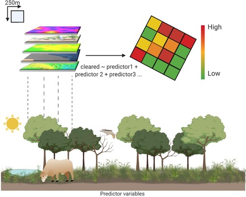
Figure 2. Schematic representation of the modelling procedure. Predictor variables listed in Table 1 were rasterised to a 250*250 m resolution and then stacked into a single dataset per bioregion. We used a generalised estimating equation to predict deforestation probability.

Model calibration

To select the most parsimonious model, we performed a variable selection method that excluded variables with an unacceptably high variance inflation factor (VIF >4) (Hair et al. 2013), highly correlated variables, and variables that were not significant predictors of clearing (p > 0.05). We created a predictive model for each bioregion’s model and ensured that all the variables included in the final model satisfied acceptable thresholds.

Diagnostics for model fit

We tested the model fit in two ways: using Pearson’s Chi-square goodness of fit and by calculating the area under the curve (AUC) (defined below). To calculate the chi-squared goodness of fit, we extracted 2,500 random samples of randomly selected 100,000 observations of the predicted (modelled) and observed (cleared or not cleared) values. For each sample, we calculated Pearson’s chi-square test statistic. We report on the average of these samples and show boxplots and histograms of the imputed p-values in the Supplementary materials. Next, we plotted the receiving operating characteristic curves (ROC) using the pROC package (Robin et al. 2011) in Rstudio (RStudio Team 2015). Sensitivity (or the probability of predicting a true positive) is plotted against 1-specificity (or false-positive probability). Model performance is considered acceptable if the curve is steep, rising steeply with the Y-axis and following the top border. The area under the curve (AUC) measures how closely the model fits the desired curve. An AUC higher than 0.7 is considered acceptable, and a value of 1.0 is considered perfect (Mandrekar 2010).

Model confidence

We calculated confidence intervals per pixel (or row within our datasets) using a nonparametric bootstrapping technique with the Boot package (Canty and Ripley 2019). Bootstrapping produces a frequency distribution by resampling the model’s predicted values 500 times for 100,000 rows of data and then calculating the sample mean per resample (Burbrink and Pyron 2008). Using these imputed means, we then extracted the standard error. The 95 per cent confidence limits were calculated by adding or subtracting the standard error of the bootstrapped mean from the predicted values’ mean and multiplying by 1.96 (Carpenter and Bithell 2000). We summarise by reporting on the 95 per cent intervals in this way: $C{I}_m=\mathrm{Mean}\pm (S{E}_{\mathrm{boot}}\ast 1.96)$Where ‘mean’ is the mean predicted clearing probability values per bioregion and ‘SE_boot’ is the standard error of the bootstrapped simulation.

Combining with vegetation community data

Next, we created spatial models of possible clearing under variable scenarios. These are not time-bound scenarios but instead can be interpreted as terminal clearing scenarios in terms of how much habitat loss might be expected over time depending on landholders’ values (for example, their appetite for agricultural activities on variable quality land) or changes in technology or land uses that facilitate use of land on lower quality areas. Once satisfied that each bioregion’s model was well-calibrated, we combined the predicted probability of clearing values for each bioregion into a single spatial dataset. We then isolated areas with the highest probability for clearing, by reclassifying predicted values for the following three scenarios: i) High amounts of clearing (the most aggressive scenario). In this scenario, values above the mean (i.e. predicted values >7 per cent and including outliers) for the whole study area were reclassified with a value of ‘1’ (i.e. likely to be cleared) and values below the mean as ‘0’ (i.e. not likely to be cleared) ii) Moderate amount of clearing. In this scenario, values above in the upper quartile (i.e. predicted values >11 per cent including outliers) for the whole study area were reclassified with a value of ‘1’ and values below the mean as ‘0’ and iii) Low amount of clearing. In this scenario, predicted probability values above the upper whisker (i.e. outliers only or predicted values >25 per cent) for the whole study area were reclassified with a value of ‘1’ and values below the mean as ‘0’.

Given assumptions around landholder behaviour and land use needs for different land capacities, these scenarios consider the range of the total extent of clearing that might occur over time. This created three binary spatial layers with values of ‘1’ denoting areas most likely to be cleared and ‘0’ denoting areas less likely to be cleared. We then used the Raster package (Hijmans et al. 2015) to create spatial grids (250m*250 m) of these binary classifications and exported them as rasters for further analysis in ArcMap 10.7 (ESRI 2014).

Queensland’s vegetation communities are mapped into ‘regional ecosystems’, constituting a world-class vegetation community dataset and is a valuable proxy for biodiversity. Regional ecosystems (Neldner et al. 2012) are mosaics of geology, landforms, and dominant vegetation. Across most of the state, Regional Ecosystems are mapped at 1:100 000, with finer scale mapping in some coastal regions including the Wet Tropics and South East Queensland (Neldner et al. 2022).

We used the most recent and comprehensive depiction of Queensland’s natural communities: version 11.1, which included mapping 1,542 regional ecosystems (Queensland Herbarium 2019). We used two regional ecosystem datasets: ‘pre-clear’ and ‘remnant.’ The first dataset is the expected distribution of a regional ecosystem in the absence of European settlement and clearing. The second refers to the current extent of the regional ecosystem. Some regional ecosystem polygons are mosaics where a maximum of five regional ecosystems could occur within a single polygon. We assumed that the area of any regional ecosystem is equal to the total polygon area multiplied by the percent of that polygon attributed to that regional ecosystem. Finally, we calculated the total area of overlap of intersecting the remnant regional ecosystem mapping with pixels classified as ‘1’ (likely to be cleared) for each of the three scenarios described above (DeCoster, Gallucci, and Iselin 2011) using the formula described in Equation 2. We also assumed that clearing was uniform in areas classified as likely to be cleared under each scenario. $\text{\%}\mathrm{remaining}={\displaystyle \frac{\mathrm{Are}{a}_{2019}-(\mathrm{Are}{a}_{\mathrm{pot}}-\mathrm{Are}{a}_{\mathrm{pa}})}{\mathrm{Are}{a}_{\mathrm{preclear}}}\ast 100}$Where the percent remaining is the proportion of the regional ecosystem’s pre-cleared (Area_prelear) extent if all potential areas (Area_pot) areas (excluding those currently under protection, Area_pa) are cleared from the current extent, Area₂₀₁₉. In this context, the area of potential clearing (Area_pot) was defined based on the three (high, moderate, and low case) scenarios described above.

Predicting a change in vegetation management status

Queensland regulates its vegetation communities by assigning a status to each regional ecosystem which signifies its vulnerability to extinction (Government 2015b). This status is relative to the amount of the regional ecosystem remaining and includes the following categories: least concern, of concern, and endangered (See supplementary for definitions in Table S1). We calculated the percent of each regional ecosystem remaining and assessed the extent remaining against the benchmarks shown in Table S1. Biodiversity status has two primary considerations: the total amount of a particular regional ecosystem remaining relative to its pre-European settlement (pre-clear) extent, and whether a particular regional ecosystem is naturally rare (i.e. has a pre-clear distribution of less than 10,000 ha). For example, a regional ecosystem is considered least concern if greater than 30 per cent of its pre-clear extent remains. If its remaining extent falls below 30 per cent and its remnant extent is greater than 10,000 ha, then it is classified as of concern.

For each scenario (low, moderate and high), we calculated the total area of overlap between each regional ecosystem and areas with a pixel value of ‘1’ (i.e. the possibility of clearing). We assumed that any pixels with a value of ‘1’ would be cleared at some point in the future. We noted any regional ecosystems that would experience one or more possible status changes. An example of one status change would be transferring from a least concern status to an of concern status. An example of two status changes would be moving from a least concern status to endangered status. In summary, the steps associated with this analysis are:

1. Calculated the total area of future clearing based on the extent to which each vegetation community overlaps with the probability of clearing scenarios described above;

2. Calculated the area likely to remain intact based on each scenario and subtracted that area from the current extent. The remaining area from this subtraction is divided by the total area before European settlement (pre-clearing).;

3. Compare the percent that is derived from step 2 with the appropriate vegetation community status (i.e. endangered if the total extent falls below 10 per cent of pre-European levels);

4. All status changes are recorded, including instances where a vegetation community will make more than one change.

For example, regional ecosystem 11.7.7 is a least concern regional ecosystem, described as a mixture of Eucalyptus and Corymbia woodlands on Cainozoic lateritic duricrust and is currently considered least concern. It has an estimated pre-European extent of 203,764 ha, but as of 2018, it had been reduced to 174,903 ha. A further 169,931 ha of this regional ecosystem occurs in areas that may be cleared according to the high scenario, and none of this regional ecosystem occurs in protected areas. Assuming full clearing with this scenario, only 4,971 ha (2 per cent of its pre-European extent) would remain. It would then be classified as an endangered, constituting two changes in status.

Results

Model fit and confidence

AUC values ranged from 0.623 (New England Tablelands) to 0.836 (Wet Tropics), indicating an acceptable model fit for all bioregions except the New England Tablelands (see ROC curves in Supplementary). We found that the confidence intervals obtained by bootstrapping had a negligible effect on the mean predictions (8.57*10⁻⁶–1.96*10⁻⁴). Considering these three tests, we conclude that our models are well-fitted to the data and that the provided predictions are reliable (Table 2) (Alsadik 2019; Ling, Huang, and Zhang 2003).

Table 2. A description of the variables included in the final model (p < 0.05) for each bioregion. ‘Built’ refers to Euclidean distance to built-up areas, ‘graze’ refers to grass biomass, ‘rain’ refers to average annual rainfall, ‘roads’ refers to Euclidean distance to State-controlled roads, ‘slope’ refers to slope in per cent rise, ‘temp’ refers to yearly average temperature, ‘wc’ refers to Euclidean distance to major watercourses. The third column shows the mean (M) of simulated Pearson’s Chi-Squared goodness-of-fit values. Chi-square tests whether or not the observed data are consistent with the values imputed from the models (Alsadik 2019). ^{^} indicates that there is no significant difference between the predicted and observed clearing data and the models have performed well. The final column is the mean (M) confidence interval (upper and lower 95 per cent of values) for each bioregion (see methods: model confidence).

Bioregion	List of covariates	M.Chi – Square	M.df	M.pvalue	M. Confidence intervals
Brigalow Belt	Built, rain, roads, slope, temp, wc	97855	97853	0.4980^^	0.103 ± 5.27*10^−5
Cape York	Graze, rain, slope, temp wc	96995	96994	0.4919^^	3.40*10^−3 ± 7.35*10^−6
Central Queensland Coast	Graze, rain, roads, slope, temp, wc	78567	78573	0.5083^^	3.697*10^–2± 1.53*10^−4
Desert Uplands	Graze, rain, roads, slope, temp, wc	95021	95017	0.4961^^	0.0910 ± 1.96*10^−4
Einasleigh Uplands	Built, graze, rain, roads, slope, temp, wc	98645	98646	0.4993^^	1.016*10^–2± 8.57*10^−6
Mulga Lands	Graze, rain, slope, temp, wc	98176	98174	0.4976^^	0.0990 ± 1.35*10^−4
New England Tablelands	Built, roads, slope, temp, wc	66508	66498	0.4918^^	0.0714 ± 1.71*10^−4
Southeast Queensland	Built, graze, roads, rain, slope, temp, wc	94595	94586	0.4921^^	0.0512 ± 7.85*10^−5
Wet Tropics	Built, graze, rain, roads, slope, temp, wc	83461	83466	0.5006^^	0.0224 ± 1.21*10^−4

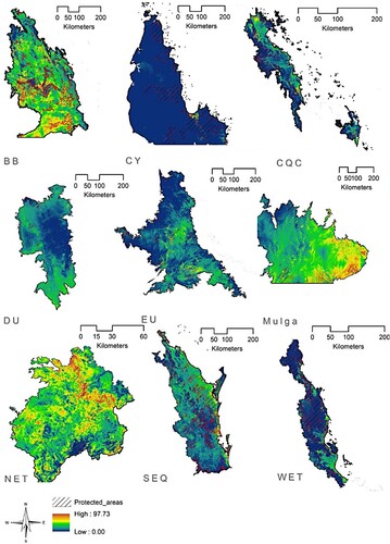
Across the study area, the probability of clearing (predicted values) ranged from 0 to 97.7 per cent, and the estimated probability of clearing in each bioregion was highly variable across regions. Higher probabilities were observed in the Brigalow Belt and Mulga Lands compared to other bioregions (97 per cent and 90 per cent respectively). Lower probabilities were more common in certain bioregions, with mean probabilities less than 1 per cent observed in the Cape York, Central Queensland Coast and Wet Tropics bioregions (Figure 3).

Figure 3. Map of the likelihood that a pixel will be cleared given the relevant biophysical characteristics of the pixel. The predicted values for each bioregion are shown in a combined raster format ‘predicted values.’BB = Brigalow Belt, CY = Cape York, CQC = Central Queensland Coast, DU = Desert Uplands, EU = Einasleigh Uplands, Mulga = Mulga Lands, NET = New England Tablelands, SEQ = Southeast Queensland, WET = Wet Tropics.

Probable clearing and impacted regional ecosystems.

The total area of overlap between the predicted clearing layer and regional ecosystems was variable across the three scenarios (i.e. low, moderate, and high).

Probable clearing: low scenario

We assumed that all areas with a modelled risk of clearing equal to or greater than 25 per cent would be cleared, meaning that clearing is assumed to occur only in highly suitable areas. This equates to 336,323 ha or 0.3 per cent of the study area. Many of these areas are in the Brigalow Belt (122,920 ha, 36.5 per cent), the Desert Uplands (119,933 ha, 35.6 per cent), and the Mulga Lands (88,744 ha, 26 per cent). The smallest areas were in the New England Tablelands (168 ha, < 0.1 per cent) and Southeast Queensland (24 ha, < 0.1 per cent). There were no areas in the Cape York, Central Queensland Coast, or Wet Tropics bioregions with a probability of clearing greater than 25 per cent.

Probable clearing: moderate scenario

We assumed all areas with a modelled risk of clearing equal to or greater than 11 per cent would be cleared. This equates to 9,124,694 ha or 9.3 per cent of the study area. Most of these areas are in the Brigalow Belt (43 per cent, 3,905,097 ha) and Mulga Lands (44 per cent 3,995,525 ha). The smallest areas observed are in the Cape York bioregion (280 ha).

Probable clearing: high scenario

We assume all areas with a modelled risk of clearing equal to or greater than 7 per cent (the most aggressive assumption allowing clearing on land with a clearing probability above the mean). This equates to 19,911,658 ha, or approximately 20 per cent of the study area (Figure 3). The majority of areas (87 per cent) with a possibility of clearing occur in the Mulga Lands (44 per cent of the bioregion, 8,944,000 ha) and Brigalow Belt (43 per cent of the bioregion, 8,307,000 ha) bioregions. The smallest areas predicted are in the Cape York and Einasleigh Uplands bioregions.

Impact of predicted clearing on regional ecosystems: high scenario

Nearly half of the currently mapped regional ecosystems (45 per cent, n = 688) overlap to some extent with the possibility of clearing under the high scenario. However, the extent of overlap in terms of the total current area of a particular regional ecosystem was highly variable, with a minimum of 1 per cent to a maximum of 100 per cent. The average area of overlap was 27 per cent. The number of regional ecosystems with an extent of overlap of less than 1 per cent of their total area was 283. We found that 158 regional ecosystems overlap to such an extent that they are likely to change the vegetation management status at least once. Most of these regional ecosystems are in the Brigalow Belt (n = 74) and Mulga Lands (n = 45), and the fewest came from the New England Tablelands (n = 5) and the Central Queensland Coast (n = 7). Furthermore, 72 regional ecosystems may experience two changes to their vegetation management status. The majority of these regional ecosystems are found in the Brigalow Belt (n = 27) and Mulga Lands (n = 31) (Table 3, Table A2).

Table 3. Summary table of the number of regional ecosystems affected in each bioregion per scenario. Number is the number of regional ecosystems affected under each of the scenarios. 1 status change is the number of regional ecosystems that will change status once and 2 status changes are those that will change status twice (i.e. from Least Concern to to Endangered) under each scenario.

	Low Scenario			Moderate Scenario			High Scenario
Bioregion	Number	1 status change	2 status changes	Number	1 status change	2 status changes	Number	1 status change	2 status changes
Brigalow Belt	114	2	–	157	30	6	166	74	27
Cape York	1	1	–	20	–	–	66	1	–
Central Queensland Coast	8	3	–	41	2	–	65	7	–
Desert Uplands	69	–	–	74	8	–	75	15	3
Einasleigh Uplands	19	1	–	51	–	–	78	–	–
Mulga Lands	40	7	–	64	29	9	64	45	31
New England Tablelands	5	–	–	13	1	–	22	4	2
Southeast Queensland	12	12	2	126	17	4	152	12	9
Total	268	26	2	546	87	19	688	158	72

Impact of overlap on regional ecosystems: moderate scenario

Over a third of Queensland’s regional ecosystems overlap with areas of moderate probability for clearing (n = 546, 35 per cent of the total number of regional ecosystems); however, the total extent of this overlap was highly variable (0 up to 99.72 per cent with an average overlap of 7.3 per cent). There were 103 regional ecosystems where less than 1 per cent of their current extent intersected with the predicted clearing layer. In this scenario, 87 (5 per cent of all regional ecosystems) regional ecosystems overlapped to such an extent that they are likely to change the vegetation management status at least once. Most of these regional ecosystems were from the Brigalow Belt (n = 30) and Mulga Lands (n = 29). The fewest likely regional ecosystem status changes were observed in the New England Tablelands (n = 1). Furthermore, 21 regional ecosystems were predicted to experience two changes in their status, with the majority of these regional ecosystems found in the Mulga Lands (n = 9) and the Brigalow Belt (n = 6) (Table 3, Table A3).

Impact of predicted clearing on regional ecosystems: low scenario

We identified 268 regional ecosystems that overlap with areas that have the potential for clearing (17.3 per cent) according to the low scenario (Table 3). The extent to which the predicted clearing layer intersected with each regional ecosystem was highly variable, ranging from 1 per cent to 26.75 per cent with an average overlap of 1.4 per cent. There were 210 regional ecosystems where less than 1 per cent of their current extent overlapped with potential clearing areas. In this scenario, 26 regional ecosystems overlapped to such an extent that they may change the vegetation management status at least once. Of these, most were from the Southeast Queensland bioregion (n = 12) and Mulga Lands bioregions (n = 7). The fewest regional ecosystems were observed in Cape York (n = 1) and Einasleigh Uplands (n = 1). We identified that two regional ecosystems could change from least concern to endangered status, both in Southeast Queensland (regional ecosystem 12.3.6 and regional ecosystem 12.3.13). Eight regional ecosystems could change from an of concern to endangered status (Table 3, Table A4).

Discussion

Estimating the potential total extent of habitat loss due to clearing is critical for designing targeted native vegetation management policies that prevent future loss (Ward et al. 2019). In Queensland, policies that utilise predictive methods, such as those presented in this study, can be effective in avoiding the loss of native remnant vegetation and preventing the transfer of vegetation communities into higher threat statuses. By predicting future impacts and implementing measures to prevent or mitigate those impacts, these interventions can protect vulnerable ecosystems and promote sustainable land use practices (Evans 2016; Synes et al. 2020).

Our analysis revealed that the number of vegetation communities impacted by future clearing ranged from 17 per cent under the low scenario to 45 per cent under the high scenario. It is important to note that this range of values highlights the need to carefully consider the threshold for reclassifying clearing probability values. In the high scenario, even probability values as low as 7 per cent were included in the binary reclassified layer, which could overestimate the potential future impact of land clearing. However, our low scenario is potentially overly restrictive, with a small area exposed to clearing. While any one scenario may be considered to have unrealistic assumptions, collectively, our three scenarios present a range of possible total areas exposed to clearing. Thus, the scenarios as a bounded range of plausible futures can provide policymakers and decision makers a bounded understanding of how much native vegetation might be exposed to, and lost from, land clearing.

Clearing risk has implications for some vegetation communities in Queensland and should accompany diverse policy interventions to target specific regional issues. The Brigalow Belt and Mulga Lands were the bioregions with the highest predicted probability of clearing (90.5 per cent, 97.7 per cent). High predicted probabilities in these regions are unsurprising because historical and modern clearance rates are high, similar to tropical clearing hotspots in South America and Southeast Asia (Lepers et al. 2005; Queensland Department of Environment and Science 2018). Indeed, since the mid-twentieth Century, mechanised clearing and a government settlement policy (the Brigalow Development Scheme) catalysed clearing for agricultural development (Seabrook, McAlpine, and Fensham 2006). This successfully established large agricultural areas in the Brigalow Belt and, subsequently, the adjacent Mulga Lands. Our results demonstrate that these bioregions may be useful targets for future clearing abatement policy as agricultural practices continue to have significant implications on landscapes within these bioregions. It may be helpful for policies to consider socio-economic drivers of clearance and target the largest farmland parcels as farmlands expand outwardly (Seabrook, McAlpine, and Fensham 2008). Predictive models, such as the one presented here, could be incorporated into risk-based approaches (Stelzenmüller et al. 2018), which combine the probabilistic risk assessment with the characteristics and exposure sequences (these could be socio-economic and policy drivers of clearing) and all factors which reduce risk (this may include regulatory instruments or socio-cultural values (Hauptmanns 2005)).

Large areas in Cape York, Central Queensland Coast and Wet Tropics Bioregions show a low risk of clearing. Concerning Cape York, we suggest that low probabilities result from the bioregions remoteness, while the other two bioregions may result from clearing saturation. Cape York is Queensland’s most remote bioregion with a relatively unmodified landscape; however, this may change if the bioregion becomes more developed and accessible. The Central Queensland Coast is among Queensland’s most heavily fragmented bioregions (Neldner et al. 2017), with historic and modern clearing transforming over 30 per cent of its area. This bioregion, however, remains a stronghold for some threatened species (Garnett, Szabo, and Dutson 2011). Australian expertise in revegetation, restoration and regeneration of landscapes would benefit this bioregion so long as the interventions have firm commitments in resourcing, appropriate scaling and proper management (Campbell, Alexandra, and Curtis 2017). The mountainous regions of the Wet Tropics are difficult and costly to clear, and most of the lowland areas have been cleared to establish sugarcane, bananas, pasture and orchard crops, thus reducing some original vegetation community types to <10 per cent of their original range (Metcalfe and Ford 2009). Our models suggest that future clearing does not directly threaten the mountainous landscapes, corroborating previous work (Queensland Department of Environment and Science 2018). However, the Wet Tropics is subject to various threatening processes, including disease, invasive species and climate change. Three significant diseases impact biodiversity in the Wet Tropics: chytridiomycosis (or chytrid fungus), myrtle rust (Puccinia psidii) and phytophthora root rot (McKnight et al. 2017; Pegg et al. 2018; Worboys 2006). All three diseases heavily impact individual vitality, and, if left uncontrolled, can negatively impact impacted species (Fensham and Radford-Smith 2021). Furthermore, there are over 60 invasive species (such as gamba grass, Andropogon gayanus), and feral cats (Felis catus) (Harrison and Congdon 2002) in the Wet Tropics Bioregion (Poon et al. 2007; Stork, Goosem, and Turton 2011). Each invasive species potentially outcompete or attack native flora and fauna, resulting in the decline of native populations. Lastly, the multiplicative effect of climate change has serious implications for biodiversity in the Wet Tropics with modulations in the climatic factors determining rainforest persistence (Williams, Bolitho, and Fox 2003). Regions highly saturated by clearing may benefit from well-resourced management and ecological restoration.

We have demonstrated that freely available datasets provide valuable insights about the trends and correlation of clearing drivers that might have otherwise been missed, and significant advances have been made in the clearing modelling literature (Wang et al. 2022). The methods applied in this constitute a well-understood and scientifically sound technique and was chosen because the models are easy to implement, and can be updated quickly as freely available datasets are updated. Such models are ideal for understanding the correlations between variables that can provide insights into the clearing drivers. However, additional techniques, including artificial neural networks (Ahmadi 2018) and Bayesian networks (Silva et al. 2019), also warrant evaluation (Mayfield et al. 2016). Tree-based methodologies (Zanella et al. 2017) have also been identified as potentially suitable candidates and have recently started appearing in clearing modelling literature (de Souza and De Marco 2018). Our models have incorporated known drivers of clearing in this context based on a comprehensive literature search. To avoid over-fitting, we have tried to limit our predictor co-variates which directly relate to climate, topography and land productivity concerning cattle grazing. Future models could consider incorporating the Queensland Government’s Agricultural Land Audit Data (2013) which describes land capability for cropping. As land capability is a function of climatic conditions and this dataset is derived using tree canopy (also used in the predictor variable), this dataset was not used. Lastly, distance to currently cleared areas could be investigated as a predictor and cost-distance to roads or markets (rather than Euclidean distance).

Clearing in portions of regional ecosystems has important implications for habitat fragmentation, one of conservation’s most studied threatening processes (Nghiem et al. 2016). Previous studies have suggested habitat fragmentation has negative impacts on biodiversity by catalysing future habitat loss (Collinge 2009), localising extinctions on patches in the presence of pathogens (McCallum and Dobson 2002), introducing edge effects, and altering nutrient cycles to ultimately reduce biodiversity by 13-75 per cent (Haddad et al. 2015). Thus, even moderate amounts of clearing on Queensland’s vegetation communities have important ecological consequences that are not yet understood. Predicting clearing before it occurs provides the opportunity to understand whether or not potential clearing will, in fact, negatively affect vegetation communities. Presently, vegetation management status is classified using the percent remaining and level of degradation (e.g. 30 per cent of historic extent), but there may be limited scientific justification or rationale to support these benchmarks. While our analysis is consistent with the thresholds provided in the regulation, we note that there may be a need to understand the viability of each regional ecosystem in terms of compounding threats (Neely et al. 2001; Pintor et al. 2019).

Furthermore, Simmons et al. (2018) found that remnant vegetation land-clearing rates increased substantially under policy reform with significant implications for biodiversity (Reside et al. 2017). When introduced too quickly, policy reforms may inadvertently drive clearing through a phenomenon termed ‘panic clearing.’(Angelsen 2009). Panic clearing is described as an individual’s response to legislative uncertainty. To prevent ‘panic clearing’ (Bartel 2004) decisions, it may be prudent to consider how clearing could impact these vegetation communities in the future using predictive modelling. (Sutherland and Freckleton 2012; Veldkamp and Lambin 2001). Our study adds to the existing knowledge of the status of biodiversity in Queensland by predicting the probability that currently forested pixels could become cleared and then estimating the risk to the status of regional ecosystems from clearing. The predictions effectively represented potential clearing across Queensland. As expected, the study identified variation in both the predictors of clearing and the maximum potential for clearing between regions.

Land clearing is driven by a variety of factors, including commercial and industrial interests, agricultural expansion, urbanisation, and infrastructure development, as well as (Parker, Hessl, and Davis 2008; Trudgill 2022). Decisions related to land use are notably shaped by these beliefs, with economic considerations playing a crucial role. While our analysis focuses on biophysical predictors of clearing and their implications for the heighted vulnerability of vegetation communities, it is important to note the absence of economic factors, human values and temporal dynamics. This limits our model from capturing the evolving nature of economic and societal influences on land clearing over time. Our estimates reflect patterns in clearing related to biophysical determinants but do not reflect temporal shifts in economic, regulatory and societal factors impacting land clearing patterns. Nevertheless, previous research has determined the strong connection between decisions to clear land and land capability (Adams and Engert 2023) and consequently our approach provides plausible future terminal views. Future research could explore scenarios of land clearing with consideration of changes to clearing rates over time concerning socio-economic and regulatory factors.

In Queensland, land clearing has been identified as a leading cause of habitat loss and biodiversity decline. While policy interventions such as the Vegetation Management Act 1999 can successfully reduce clearing rates, the potential for switft policy changes looms amid economic pressures and changing political priorities (Maron et al. 2015). The identification of vulnerable vegetation communities offers crucial insights to guide policy decisions, especially in devising interventions that protect regional ecosystems from escalated clearing following rapid policy changes. The outcomes of this research can serve as a foundation for supporting policy interventions aimed at preserving ecosystems and promoting sustainable land use practices throughout Queensland. By incorporating these findings into policymaking processes, decision-makers can strategically target interventions to areas where they are most crucial, thereby fostering more effective conservation outcomes.

Acknowledgement

The authors would like to acknowledge the valuable contributions of each team member to the design, analysis, and writing of this manuscript. Vanessa Adams and Stephanie Hernandez conceptualised the study. All authors developed the research questions, and designed the methodology. Stephanie Hernandez completed the data collection, data analysis, and interpretation of the results. Nicholas Murray, Stephanie Duce and Vanessa Adams provided expertise in spatial analysis and policy analysis and contributed to the development and implementation of research. Marcus Sheaves provided supervisory support and contributed to the statistical analysis. All authors contributed to the writing of the manuscript. Stephanie Hernandez conducted extensive literature reviews, coordinated discussions with Queensland’s Department of Environment and Science to ensure the accuracy of the interpretation of regional ecosystem identifications. The Authors acknowledge Peter Johnson who provided critical insights and expertise in the field of vegetation management and contributed to the interpretation of the findings. All authors actively participated in the writing and revision process, providing intellectual input, and approving the final version of the manuscript.

Disclosure statement

No potential conflict of interest was reported by the author(s).

Additional information

Funding

This work was supported by Queensland State Government: [Grant Number 201600768].

References

- Accad, A., and V. J. Neldner. 2015. Queensland Department of Science, Information Technology and Innovation: Brisbane, Qld.
- Adams, Vanessa M, and Jayden E Engert. 2023. “Australian Agricultural Resources: A National Scale Land Capability map.” Data in Brief 46: 108852. https://doi.org/10.1016/j.dib.2022.108852
- Adeboye, Oyelola A, Denis HY Leung, and You-Gan Wang. 2018. “Analysis of Spatial Data with a Nested Correlation Structure: An Estimating Equations Approach.” Journal of the Royal Statistical Society: Series C: Applied Statistics 67 (2): 329–354.
- Aguiar, Ana Paula Dutra, Gilberto Câmara, and Maria Isabel Sobral Escada. 2007. “Spatial Statistical Analysis of Land-use Determinants in the Brazilian Amazonia: Exploring Intra-Regional Heterogeneity.” Ecological Modelling 209 (2–4): 169–188. https://doi.org/10.1016/j.ecolmodel.2007.06.019.
- Ahmadi, Vahid. 2018. “Using GIS and Artificial Neural Network for Deforestation Prediction”.
- Alsadik, Bashar. 2019. “Chapter 12 - Postanalysis in Adjustment Computations.” In Adjustment Models in 3D Geomatics and Computational Geophysics, edited by Bashar Alsadik, 345–385. Amsterdam, Netherlands: Elsevier.
- Angelsen, Arild. 2009. Realising REDD+: National Strategy and Policy Options. Vol. 1, 125–138.
- ESRI. 2014. ArcMap 10.2.1. ESRI (Environmental Systems Resource Institute), Redlands, California.
- Bartel, Robyn L. 2004. “Satellite Imagery and Land Clearance Legislation: A Picture of Regulatory Efficacy?” Australasian Journal of Natural Resources Law and Policy 9 (1): 1.
- Bradshaw, Corey JA. 2012. “Little Left to Lose: Deforestation and Forest Degradation in Australia Since European Colonization.” Journal of Plant Ecology 5 (1): 109–120. https://doi.org/10.1093/jpe/rtr038
- Burbrink, Frank T, and R. Alexander Pyron. 2008. “The Taming of the Skew: Estimating Proper Confidence Intervals for Divergence Dates.” Systematic Biology 57 (2): 317–328. https://doi.org/10.1080/10635150802040605.
- Campbell, Andrew, Jason Alexandra, and David Curtis. 2017. “Reflections on Four Decades of Land Restoration in Australia.” The Rangeland Journal 39 (6): 405–416. https://doi.org/10.1071/RJ17056
- Canty, Angelo, and Brian Ripley. 2019. Package ‘boot’. Version.
- Carpenter, James, and John Bithell. 2000. “Bootstrap Confidence Intervals: When, Which, What? A Practical Guide for Medical Statisticians.” Statistics in Medicine 19 (9): 1141–1164. https://doi.org/10.1002/(SICI)1097-0258(20000515)19:9<1141::AID-SIM479>3.0.CO;2-F
- Carwardine, Josie, Trudy O'Connor, Sarah Legge, Brendan Mackey, Hugh P. Possingham, and Tara G. Martin. 2012. “Prioritizing Threat Management for Biodiversity Conservation.” Conservation Letters 5 (3): 196–204.
- Ceballos, Gerardo, and Paul R Ehrlich. 2002. “Mammal Population Losses and the Extinction Crisis.” Science 296 (5569): 904–907. https://doi.org/10.1126/science.1069349
- Chen, Jien, and Nicole A. Lazar. 2012. “Selection of Working Correlation Structure in Generalized Estimating Equations via Empirical Likelihood.” Journal of Computational and Graphical Statistics 21 (1): 18–41. https://doi.org/10.1198/jcgs.2011.09128.
- Chomitz, Kenneth, and David A Gray. 1999. Roads, Lands, Markets, and Deforestation: A Spatial Model of Land use in Belize. Routledge: The World Bank.
- Cogger, H., H. Ford, C. Johnson, J. Holman, and D. Butler. 2003. “Impacts of Land Clearing on Australian Wildlife in Queensland,.(World Wide Fund for Nature Australia: Sydney)”.
- Collinge, Sharon K. 2009. Ecology of Fragmented Landscapes. Baltimore: JHU Press.
- DeCoster, Jamie, Marcello Gallucci, and Anne-Marie R Iselin. 2011. “Best Practices for Using Median Splits, Artificial Categorization, and Their Continuous Alternatives.” Journal of Experimental Psychopathology 2 (2): 197–209. https://doi.org/10.5127/jep.008310
- Department of Science, Information Technology and Innovation. 1988-2016. State Wide Land And Trees Study (SLATS). Dutton park, Queensland 4102: Queensland Government.
- de Souza, Rodrigo Antônio, and Paulo De Marco. 2018. “Improved Spatial Model for Amazonian Deforestation: An Empirical Assessment and Spatial Bias Analysis.” Ecological Modelling 387: 1–9. https://doi.org/10.1016/j.ecolmodel.2018.08.015.
- Dowle, Matt, Arun Srinivasan, Jan Gorecki, Michael Chirico, Pasha Stetsenko, Tom Short, Steve Lianoglou, Eduard Antonyan, Markus Bonsch, and Hugh Parsonage. 2019. “Package ‘data. table’.” Extension of ‘data. frame. ArcMap 10.2.1. ESRI (Environmental Systems Resource Institute), Redlands, California.
- Evans, Megan C. 2016. “Deforestation in Australia: Drivers, Trends and Policy Responses.” Pacific Conservation Biology 22 (2): 130–150. https://doi.org/10.1071/PC15052
- Evans, Megan C., James E. M. Watson, Richard A. Fuller, Oscar Venter, Simon C. Bennett, Peter R. Marsack, and Hugh P. Possingham. 2011. “The Spatial Distribution of Threats to Species in Australia.” BioScience 61 (4): 281–289.
- Fensham, Roderick J, and Julian Radford-Smith. 2021. “Unprecedented Extinction of Tree Species by Fungal Disease.” Biological Conservation 261: 109276.
- Garnett, Stephen, Judit Szabo, and Guy Dutson. 2011. The Action Plan for Australian Birds 2010. Melbourne: CSIRO publishing.
- Gosho, Masahiko. 2014. “Criteria to Select a Working Correlation Structure for the Generalized Estimating Equations Method in SAS.” Journal of Statistical Software 57 (1): 1–10.
- Haddad, Nick M, Lars A Brudvig, Jean Clobert, Kendi F Davies, Andrew Gonzalez, Robert D Holt, Thomas E Lovejoy, Joseph O Sexton, Mike P Austin, and Cathy D Collins. 2015. “Habitat Fragmentation and its Lasting Impact on Earth’s Ecosystems.” Science Advances 1 (2): e1500052. https://doi.org/10.1126/sciadv.1500052
- Hair, Joseph F, William C Black, Barry J Babin, and Rolph E Anderson. 2013. Multivariate Data Analysis: Pearson new International Edition. 8th ed. Upper Saddle River: Pearson Higher Ed.
- Harrison, Debra A, and Bradley C Congdon. 2002. Wet Tropics Vertebrate Pest Risk Assessment Scheme. Cairns: Cooperative Research Centre for Tropical Rainforest Ecology and Management … .
- Hauptmanns, Ulrich. 2005. “A Risk-Based Approach to Land-use Planning.” Journal of Hazardous Materials 125 (1–3): 1–9. https://doi.org/10.1016/j.jhazmat.2005.05.015.
- Heagney, E. C., Daniel S Falster, and M. Kovač. 2021. “Land Clearing in South-Eastern Australia: Drivers, Policy Effects and Implications for the Future.” Land Use Policy 102: 105243. https://doi.org/10.1016/j.landusepol.2020.105243
- Hijmans, Robert J, Steven Phillips, John Leathwick, Jane Elith, and Maintainer Robert J Hijmans. 2017. “Package ‘Dismo’.” Circles 9 (1): 1–68.
- Hijmans, Robert J, Jacob van Etten, Joe Cheng, Matteo Mattiuzzi, Michael Sumner, Jonathan A Greenberg, Oscar Perpinan Lamigueiro, Andrew Bevan, Etienne B Racine, and Ashton Shortridge. 2015. “Package ‘raster’.” R package.
- Holland, Greg J, and Andrew F Bennett. 2010. “Habitat Fragmentation Disrupts the Demography of a Widespread Native Mammal.” Ecography 33 (5): 841–853. https://doi.org/10.1111/j.1600-0587.2010.06127.x
- Hubbard, Alan E, Jennifer Ahern, Nancy L Fleischer, Mark Van der Laan, Sheri A Satariano, Nicholas Jewell, Tim Bruckner, and William A Satariano. 2010. “To GEE or not to GEE: Comparing Population Average and Mixed Models for Estimating the Associations Between Neighborhood Risk Factors and Health.” Epidemiology, 467–474. https://doi.org/10.1097/EDE.0b013e3181caeb90
- Hudson, Marc. 2019. “‘A Form of Madness’: Australian Climate and Energy Policies 2009–2018.” Environmental Politics 28 (3): 583–589. https://doi.org/10.1080/09644016.2019.1573522
- Imai, Kosuke, Gary King, and Olivia Lau. 2009. Zelig: Everyone’s Statistical Software. R Package Version 3. http://zeligproject.org/
- IPBES. 2019. “Summary for Policymakers of the Global Assessment Report on Biodiversity and Ecosystem Services of the Intergovernmental Science-Policy Platform on Biodiversity and Ecosystem Services.” [WWW Document].
- Lepers, Erika, Eric F Lambin, Anthony C Janetos, Ruth DeFries, Frédéric Achard, Navin Ramankutty, and Robert J Scholes. 2005. “A Synthesis of Information on Rapid Land-Cover Change for the Period 1981–2000.” BioScience 55 (2): 115–124. https://doi.org/10.1641/0006-3568(2005)055[0115:ASOIOR]2.0.CO;2
- Ling, Charles X, Jin Huang, and Harry Zhang. 2003. “AUC: A Statistically Consistent and More Discriminating Measure Than Accuracy.” Ijcai 3: 519–524.
- Ludeke, Aaron Kim, Robert C. Maggio, and Leslie M. Reid. 1990. “An Analysis of Anthropogenic Deforestation Using Logistic Regression and GIS.” Journal of Environmental Management 31 (3): 247–259. https://doi.org/10.1016/S0301-4797(05)80038-6.
- Mandrekar, Jayawant N. 2010. “Receiver Operating Characteristic Curve in Diagnostic Test Assessment.” Journal of Thoracic Oncology 5 (9): 1315–1316. https://doi.org/10.1097/JTO.0b013e3181ec173d.
- Maron, Martine, W. Laurance, R. Pressey, Carla P Catterall, James Watson, and Jonathan Rhodes. 2015. “Land clearing in Queensland triples after policy ping pong.” Retrieved from The Conversation: http://theconversation. com/land-clearing-in-queensland-triples-after-policy-ping-pong-38279.
- Maron, Martine, Jonathan R Rhodes, and Philip Gibbons. 2013. “Calculating the Benefit of Conservation Actions.” Conservation Letters 6 (5): 359–367. https://doi.org/10.1111/conl.12007
- Mayfield, Helen, Carl Smith, Marcus Gallagher, Lauren Coad, and Marc Hockings. 2016. “Using Machine Learning to Make the Most out of Free Data: A Deforestation Case Study”.
- McAlpine, Clive A, A. Etter, Philip M Fearnside, Leonie Seabrook, and William F Laurance. 2009. “Increasing World Consumption of Beef as a Driver of Regional and Global Change: A Call for Policy Action Based on Evidence from Queensland (Australia), Colombia and Brazil.” Global Environmental Change 19 (1): 21–33. https://doi.org/10.1016/j.gloenvcha.2008.10.008
- McCallum, Hamish, and Andy Dobson. 2002. “Disease, Habitat Fragmentation and Conservation.” Proceedings of the Royal Society of London. Series B: Biological Sciences 269 (1504): 2041–2049. https://doi.org/10.1098/rspb.2002.2079
- McKnight, Donald T, Ross A Alford, Conrad J Hoskin, Lin Schwarzkopf, Sasha E Greenspan, Kyall R Zenger, and Deborah S Bower. 2017. “Fighting an Uphill Battle: The Recovery of Frogs in Australia’s Wet Tropics.” Ecology 98 (12): 3221–3223. https://doi.org/10.1002/ecy.2019
- Metcalfe, Daniel J, and Andrew J Ford. 2009. Living in a Dynamic Tropical Forest Landscape, 123–132. Malden: Blackwell Publishing.
- Mets, Kristjan D, Dolors Armenteras, and Liliana M Dávalos. 2017. “Spatial Autocorrelation Reduces Model Precision and Predictive Power in Deforestation Analyses.” Ecosphere (Washington, D C) 8 (5): e01824.
- Neely, B., P. Comer, C. Moritz, M. Lammert, R. Rondeau, C. Pague, G. Bell, H. Copeland, J. Humke, and S. Spackman. 2001. “Southern Rocky Mountains: An ecoregional assessment and conservation blueprint.” Prepared by the Nature Conservancy with support from the USDA Forest Service, Rocky Mountain Region, Colorado Division of Wildlife, and Bureau of Land Management.
- Neldner, V. J., Melinda Laidlaw, Keith R. McDonald, Michael T. Mathieson, Rhonda Melzer, W. J. F. McDonald, C. J. Limpus, Rod Hobson, and Richard Seaton. 2017. Scientific Review of the Impacts of Land Clearing on Threatened Species in Queensland. Brisbane: Department of Science, Information Technology and Innovation.
- Neldner, V. J., B. A. Wilson, H. A. Dillewaard, T. S. Ryan, D. W. Butler, W. J. F. McDonald, D. Richter, E. P. Addicott, and C. N. Appelman. 2022. Methodology for surveying and mapping regional ecosystems and vegetation communities in Queensland Version 6.0. edited by Science and Technology Division Queensland Herbarium. Department of Environment and Science PO Box 5078 Brisbane QLD 4001: The State of Queensland (Department of Environment and Science).
- Neldner, V. J., B. A. Wilson, E. J. Thompson, and H. A. Dillewaard. 2012. Methodology for Survey and Mapping of Regional Ecosystems and Vegetation Communities in Queensland, Version 3.2 August 2012. Brisbane: Queensland Herbarium, Department of Science, Information Technology, Innovation and the Arts.
- Nghiem, Le T. P., Sarah K. Papworth, Felix K. S. Lim, and Luis R. Carrasco. 2016. “Analysis of the Capacity of Google Trends to Measure Interest in Conservation Topics and the Role of Online News.” PLoS One 11 (3): e0152802.
- Nori, Javier, Julián N. Lescano, Patricia Illoldi-Rangel, Nicolás Frutos, Mario R. Cabrera, and Gerardo C. Leynaud. 2013. “The Conflict Between Agricultural Expansion and Priority Conservation Areas: Making the Right Decisions Before it is Too Late.” Biological Conservation 159: 507–513. https://doi.org/10.1016/j.biocon.2012.11.020.
- Parker, Dawn C, Amy Hessl, and Sarah C Davis. 2008. “Complexity, Land-use Modeling, and the Human Dimension: Fundamental Challenges for Mapping Unknown Outcome Spaces.” Geoforum; Journal of Physical, Human, and Regional Geosciences 39 (2): 789–804. https://doi.org/10.1016/j.geoforum.2007.05.005
- Pegg, Geoff, Angus Carnegie, Fiona Giblin, and Suzy Perry. 2018. Managing Myrtle Rust in Australia. Brisbane: Plant Biosecurity Cooperative Research Centre.
- Pintor, Anna, Mark Kennard, Jorge Álvarez-Romero, and Stephanie Hernandez. 2019. “Prioritising Threatened Species and Threatening Processes across Northern Australia: User Guide for Data”.
- Poon, E., D. A. Westcott, D. Burrows, and A. Webb. 2007. “Assessment of research needs for the management of invasive species in the terrestrial and aquatic ecosystems of the Wet Tropics.” Report to the Marine and Tropical Sciences Research Facility. Reef and Rainforest Research Centre Limited. Cairns.
- Pressey, Robert L, Piero Visconti, Madeleine C McKinnon, Georgina G Gurney, Megan D Barnes, Louise Glew, and Martine Maron. 2021. “The Mismeasure of Conservation.” Trends in Ecology & Evolution 36 (9): 808–821. https://doi.org/10.1016/j.tree.2021.06.008
- Queensland Department of Environment and Science. 2018. Land Cover Change in Queensland Statewide Landcover and Trees Study Summary Report: 2016–17 and 2017–18. In SLATS, edited by Department of Environment and Science. Brisbane, Queensland.
- Queensland Government. 2013. Queensland Agriculture Land Audit edited by Fisheries Department of Agriculture, and Forestsry. Brisbane Queensland: Queensland Government.
- Queensland Government. 2015a. Land Cover Change in Queensland 2014–15: a Statewide Landcover and Trees Study (SLATS) report. edited by Information Technology and Innovation Department of Science. Brisbane, Queensland.
- Queensland Government. 2015b. Vegetation Management Act 1999. edited by Queensland Parliamentarty Counsel. Brisbane.
- Queensland Government. 2017. Biodiversity Status of Pre-clearing and 2015 Remnant Regional Ecosystems - version 10.0. edited by Department of Science Information Technology and Innovation. Queensland Spatial Catalogue.
- Queensland Government. 2018. Data Summaries 1988–2018 edited by Department of Environment and Science. Open Data Portal.
- Queensland Government. 2018. Queensland Spatial Catalogue—QSpatial. Brisbane: Queensland State Government. Retrieved from: https://qldspatial.information.qld.gov.au/catalogue/custom/index.page.
- Queensland Herbarium. 2019. Regional Ecosystem Description Database (REDD). Version 11.1. edited by DES: Brisbane.
- Reside, April E, Jutta Beher, Anita J Cosgrove, Megan C Evans, Leonie Seabrook, Jennifer L Silcock, Amelia S Wenger, and Martine Maron. 2017. “Ecological Consequences of Land Clearing and Policy Reform in Queensland.” Pacific Conservation Biology 23 (3): 219–230. https://doi.org/10.1071/PC17001
- Rhodes, Jonathan R, Lorenzo Cattarino, Leonie Seabrook, and Martine Maron. 2017. “Assessing the Effectiveness of Regulation to Protect Threatened Forests.” Biological Conservation 216: 33–42. https://doi.org/10.1016/j.biocon.2017.09.020
- Robin, Xavier, Natacha Turck, Alexandre Hainard, Natalia Tiberti, Frédérique Lisacek, Jean-Charles Sanchez, and Markus Müller. 2011. “pROC: An Open-Source Package for R and S+ to Analyze and Compare ROC Curves.” BMC Bioinformatics 12 (1): 77. https://doi.org/10.1186/1471-2105-12-77
- RStudio Team. 2015. RStudio: Integrated Development for R. Boston, MA: RStudio, Inc. http://www. rstudio. com 42:14.
- Seabrook, Leonie, Clive McAlpine, and Rod Fensham. 2006. “Cattle, Crops and Clearing: Regional Drivers of Landscape Change in the Brigalow Belt, Queensland, Australia, 1840–2004.” Landscape and Urban Planning 78 (4): 373–385. https://doi.org/10.1016/j.landurbplan.2005.11.007
- Seabrook, Leonie, Clive McAlpine, and Rod Fensham. 2008. “What Influences Farmers to Keep Trees?: A Case Study from the Brigalow Belt, Queensland, Australia.” Landscape and Urban Planning 84 (3-4): 266–281. https://doi.org/10.1016/j.landurbplan.2007.08.006
- Silva, Alexsandro C. O., Leila M. G. Fonseca, Thales S. Körting, and Maria Isabel S. Escada. 2019. “A Spatio-Temporal Bayesian Network Approach for Deforestation Prediction in an Amazon Rainforest Expansion Frontier.” Spatial Statistics 35: 100393.
- Simmons, B. Alexander, Elizabeth A. Law, Raymundo Marcos-Martinez, Brett A. Bryan, Clive McAlpine, and Kerrie A. Wilson. 2018. “Spatial and Temporal Patterns of Land Clearing During Policy Change.” Land use Policy 75: 399–410. https://doi.org/10.1016/j.landusepol.2018.03.049
- Stelzenmüller, Vanessa, Marta Coll, Antonios D. Mazaris, Sylvaine Giakoumi, Stelios Katsanevakis, Michelle E Portman, Renate Degen, Peter Mackelworth, Antje Gimpel, and Paolo G Albano. 2018. “A Risk-Based Approach to Cumulative Effect Assessments for Marine Management.” Science of the Total Environment 612: 1132–1140. https://doi.org/10.1016/j.scitotenv.2017.08.289
- Stork, Nigel E., Steve Goosem, and Stephen M. Turton. 2011. “Status and Threats in the Dynamic Landscapes of Northern Australia’s Tropical Rainforest Biodiversity Hotspot: The Wet Tropics.” In Biodiversity Hotspots, edited by Frank E. Zachos and Hanbel Jan Christian, 311–332. Berlin: Springer.
- Sutherland, William J., and Robert P. Freckleton. 2012. “Making Predictive Ecology More Relevant to Policy Makers and Practitioners.” Philosophical Transactions of the Royal Society B: Biological Sciences 367 (1586): 322–330. 10.1098rstb.2011.0181.
- Synes, Nicholas W, Aurore Ponchon, Stephen CF Palmer, Patrick E Osborne, Greta Bocedi, Justin MJ Travis, and Kevin Watts. 2020. “Prioritising Conservation Actions for Biodiversity: Lessening the Impact from Habitat Fragmentation and Climate Change.” Biological Conservation 252: 108819. https://doi.org/10.1016/j.biocon.2020.108819
- Taylor, Martin Francis James. 2013. Bushland at Risk of Renewed Clearing in Queensland. Brisbane: World Wildlife Fund Australia.
- Thackway, Richard, and Ian D Cresswell. 1997. “A Bioregional Framework for Planning the National System of Protected Areas in Australia.” Natural Areas Journal 17 (3): 241–247.
- Tilman, David, Michael Clark, David R. Williams, Kaitlin Kimmel, Stephen Polasky, and Craig Packer. 2017. “Future Threats to Biodiversity and Pathways to Their Prevention.” Nature 546 (7656): 73. https://www.nature.com/articles/nature22900#supplementary-information.
- Trudgill, Stephen. 2022. Why Conserve Nature?: Perspectives on Meanings and Motivations. Cambridge: Cambridge University Press.
- Tulloch, Ayesha I. T., Megan D. Barnes, Jeremy Ringma, Richard A. Fuller, and James E. M. Watson. 2015. “Understanding the Importance of Small Patches of Habitat for Conservation.” Journal of Applied Ecology 53 (2): 418–429.
- Veldkamp, Antonie, and Eric F. Lambin. 2001. Predicting Land-use Change 85 (3): 1–6.
- Wang, Ming. 2014. “Generalized Estimating Equations in Longitudinal Data Analysis: A Review and Recent Developments.” Advances in Statistics 2014: 1–11.
- Wang, Junye, Michael Bretz, M Ali Akber Dewan, and Mojtaba Aghajani Delavar. 2022. “Machine Learning in Modelling Land-use and Land Cover-Change (LULCC): Current Status, Challenges and Prospects.” Science of The Total Environment 822: 153559.
- Ward, Michelle S, Jeremy S Simmonds, April E Reside, James EM Watson, Jonathan R Rhodes, Hugh P Possingham, James Trezise, Rachel Fletcher, Lindsey File, and Martin Taylor. 2019. “Lots of Loss with Little Scrutiny: The Attrition of Habitat Critical for Threatened Species in Australia.” Conservation Science and Practice 1 (11): e117. https://doi.org/10.1111/csp2.117
- Williams, Stephen E, Elizabeth E Bolitho, and Samantha Fox. 2003. “Climate Change in Australian Tropical Rainforests: An Impending Environmental Catastrophe.” Proceedings of the Royal Society of London. Series B: Biological Sciences 270 (1527): 1887–1892. https://doi.org/10.1098/rspb.2003.2464
- Wilson, B. A., V. J. Neldner, and A. Accad. 2002. “The Extent and Status of Remnant Vegetation in Queensland and its Implications for Statewide Vegetation Management and Legislation.” The Rangeland Journal 24 (1): 6–35. https://doi.org/10.1071/RJ02001
- Wilson, Kerrie, Robert L Pressey, Adrian Newton, Mark Burgman, Hugh Possingham, and Chris Weston. 2005. “Measuring and Incorporating Vulnerability Into Conservation Planning.” Environmental Management 35 (5): 527–543. https://doi.org/10.1007/s00267-004-0095-9
- Woinarski, John C. Z., Andrew A. Burbidge, and Peter L. Harrison. 2015. “Ongoing Unraveling of a Continental Fauna: Decline and Extinction of Australian Mammals Since European Settlement.” Proceedings of the National Academy of Sciences 112 (15): 4531–4540. https://doi.org/10.1073/pnas.1417301112.
- Worboys, Stuart. 2006. Guide to Monitoring Phytophthora-Related Dieback in the Wet Tropics of North Queensland. Cairns: Cooperative Research Centre for Tropical Rainforest Ecology and Management.
- Zanella, Lisiane, Andrew M. Folkard, George Alan Blackburn, and Luis MT Carvalho. 2017. “How Well Does Random Forest Analysis Model Deforestation and Forest Fragmentation in the Brazilian Atlantic Forest?” Environmental and Ecological Statistics 24 (4): 529–549. https://doi.org/10.1007/s10651-017-0389-8
- Zorn, Christopher JW. 2001. “Generalized Estimating Equation Models for Correlated Data: A Review with Applications.” American Journal of Political Science, 470–490. https://doi.org/10.2307/2669353