Co-occurrence and abundance of pollinators and pests in horticultural systems in Africa using an integrated Earth observation-based approach

ABSTRACT

Flower-visiting insects that are pollinators play a critical role in promoting biodiversity in agroecosystems and agricultural food production through their pollination ecosystem service. However, several factors affect the survival of these pollinators and flower visitors, including the heavy and indiscriminate application of agrochemicals to control crop insect pests, which is impacted by various cropping patterns in a landscape and by shifting environmental conditions. Thus, this study focused on investigating the influence of cropping patterns on the spatial distribution of pollinators (Apis mellifera, Hymenoptera other than A. mellifera, and Syrphidae), flower visitors (Calliphoridae), and pests, i.e. fruit fly (Bactrocera dorsalis) and false codling moth (Thaumatotibia leucotreta) of the avocado, a pollinator-dependent crop. Cropping patterns, earth observation data and relevant environmental variables were used as the predictor variables for modeling the potential distribution and abundance of avocado pollinators, flower visitors and pests in one of the leading regions in avocado production in Kandara, Maragua, and Gatanga sub-Counties in Murang’a County, Kenya. In specific, species distribution modeling (SDM) and species abundance modeling (SAM) techniques, i.e. the maximum entropy (MaxEnt) model (presence-only data) and negative binomial (NB) distribution in a generalized linear model (GLM) (abundance data) were used, respectively. Additionally, the spatial distribution probability of the co-occurrence of the pollinators, flower visitors and pests was also analyzed. This study revealed that cropping patterns was the most consistent influential predictor variables for the distribution of avocado pollinators, flower visitors and pests. A large area of Kandara and some parts of Maragua and Gatanga sub-Counties showed a high spatial distribution probability of the studied avocado pollinators, flower visitors and pests. However, only the majority of Kandara sub-County had a high spatial distribution probability score of the potential co-occurrence of the avocado pollinators, flower visitors and pests. Further, A. mellifera was the most abundant flower-visiting pollinator compared with the other studied pollinators, while B. dorsalis was the most abundant avocado pest compared with T. leucotreta. In addition, GLM analysis indicated that no environmental variable was significant in explaining the abundance of the studied avocado pollinators, whereas precipitation and elevation derivatives of aspect and hillshade were statistically significant (p ≤ 0.05) in explaining the abundance of B. dorsalis. Solar radiation was significant in explaining only the abundance of T. leucotreta. Our study revealed that SDM and SAM modeling outputs can be used to inform decision-making for the implementation of sustainable management efforts regarding pollinators, flower visitors, and insect pests.

KEYWORDS:

• Avocado
• Kenya
• flower visitors
• species distribution modeling

1. Introduction

Biotic and abiotic pollination is an essential ecosystem service that accounts for 9.5% of the value of all food produced globally (Potts et al. 2010). Recent studies on the economic value of pollination provided by biotic pollinators estimated its worldwide value to be USD 195 billion to ~USD 387 billion yearly (modified for inflation in March 2020) (Porto et al. 2020). Moreover, of the 115 most important global food crops, 87 depend on insects and other animal pollinators for the production of fruits, vegetables or seeds (Klein et al. 2007).

Some studies have referred to a possible decline of these pollinators in various geographical setups (Novais et al. 2016; Rhodes 2018), while other studies have shown that managed bees are on the increase in different set-ups, as estimated from Food and Agriculture Organization (FAO) of the United Nations datasets from 1961 to 2017 (Phiri, Fèvre, and Hidano 2022). However, these insect pollinators are still endangered by factors such as landscape simplification, increasingly influenced by monoculture cropping systems; intensive use of agrochemicals such as synthetic pesticides; climate variability; and increased occurrence of pollinator pests and diseases (Moreaux et al. 2022).

Flower-visiting insects have been used to serve as an indication of pollination services in several crops, including avocado (Persea americana) (Garibaldi et al. 2020). Various insects visit the avocado flower; however, the insect flower visitors that have been known to be the most efficient pollinators for avocado are the Western honeybee Apis mellifera (Dymond et al. 2021). Consequently, distinguishing pollinators from other generic flower visitors is important in avocado production for the successful management of key pollinator species (Sagwe et al. 2022).

Avocado, a highly pollinator-dependent crop, is a vital horticultural commodity in Kenya and is largely cultivated by small-scale farmers. Eighty percent of avocado produced in Kenya is consumed in the domestic market, while the rest is exported as fresh or processed fruits/oils (Kathula 2021). However, the presence of insect pests like the false codling moth (Thaumatotibia leucotreta) and the oriental fruit fly Bactrocera dorsalis has a severe impact on the production of avocado in Kenya (Toukem et al. 2020). Integrated pest management (IPM) has been implemented in avocado production systems to combat these pests while limiting the use of chemical pesticides (Onsomu 2019), but excluding pollinator management strategies. Nevertheless, the inclusion of pollinator management strategies through integrated pest and pollinator management (IPPM) would improve yields of pollinator-dependent crops, while sustaining biodiversity (Biddinger and Rajotte 2015).

Spatial characterization of pollinators, flower visitors and pests is an essential cornerstone of IPPM. Currently, up-to-date spatial prediction of fruit crop pollinators, flower visitors and pests is scarce in agriculture-promising countries like Kenya. To the best of our knowledge, only a few studies have assessed the spatial pattern of fruit crop insect pollinators, flower visitors and pests at a localized scale. For instance, Makori et al. (2022) used multisource spatial data to understand the spatial distribution and change patterns of stingless bees in Kenya and revealed a higher probability of their decline than of their proliferation. In another study, Mandela et al. (2018) analyzed the diversity and abundance of camphor basil (Ocimum kilimandscharicum) flower visitors in Kakamega forest in Kenya and reported that species diversity of the flower visitors increased with closeness to the forest edge.

Additionally, Zingore et al. (2020) predicted the potential expansion of the peach fruit fly Bactrocera zonata and found that, under changing climatic conditions, the pest could invade wider regions in Africa and South America. Furthermore, Mahmoud et al. (2020) determined the habitat suitability of two fruit fly species (i.e. B. zonata and B. dorsalis) and their suitable co-occurrence range in Sudan, and found that the two pests were spread across a wide area in the country. Furthermore, Stotter (2009) assessed the spatial-temporal distribution of the T. leucotreta in South Africa in the citrus crop and found that male T. leucotreta were mostly confined to citrus orchards, thus providing insights into the local distribution of the T. leucotreta across the agricultural landscape. Statistical models have also been employed to estimate B. dorsalis and T. leucotreta abundance in avocado orchards by using climatic variables (Odanga et al. 2018) and a landscape productivity indicator (i.e. normalized difference vegetation index: NDVI) (Toukem et al. 2020). Both studies demonstrated the importance of climatic and NDVI variables in estimating B. dorsalis and T. leucotreta abundance, respectively. The spatial distribution of pollinators, flower visitors, and pests is also influenced by the landscape structure, which could be tailored in terms of land use land cover (LULC) or cropping patterns (Mudereri et al. 2020; Ochungo et al. 2019).

Although various milestones have been achieved by earlier studies, most have not predicted spatial distribution probability for the avocado pollinators, flower visitors, and pests in a localized avocado production system such as Murang’a County. Furthermore, few studies have assessed the use of geospatial modeling approaches for determining the suitable sites for the co-occurrence of two or more pollinators, flower visitors, or pest species (Mahmoud et al. 2020). Moreover, studies have not looked at the role or effect of remotely sensed cropping patterns and environmental variables in estimating pollinator, flower visitor and pest distribution, co-occurrence and/or abundance.

Therefore, this study sought to illustrate the synergy provided by remotely sensed outputs, e.g. cropping patterns in applications such as insect studies. Specifically, the aim of this study was twofold: (1) to predict the spatial distribution probability of avocado pollinators, flower visitors, and pests using cropping patterns, and environmental and topographic variables, together with an ecological niche modeling approach (maximum entropy: MaxEnt), and to determine the suitable co-occurrence range of the avocado pollinators, flower visitors and pests; and (2) to estimate and analyze the abundance of avocado pollinators, flower visitors and pests using environmental variables and generalized linear models (GLMs).

2. Material and methods

2.1. Study area

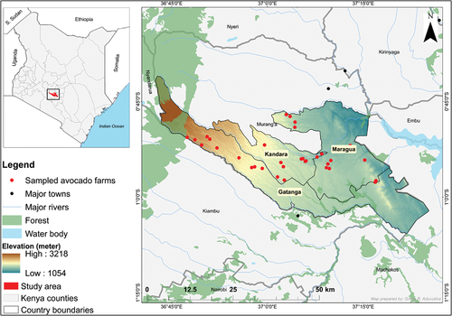
The study was conducted in the County of Murang’a in Kenya (Figure 1). The County lies between latitudes 0° 34’ 00’’ S and 1° 07’ 00’’ S, and longitudes 36° 00’ 00’’ E and 37° 27’ 00’’E. There are two distinct rainfall patterns in the area: long rains from March to May and short rains from October to November every year. The annual temperature ranges from 12°C to 20°C, while the annual rainfall ranges from 800 to 2600 mm (Ovuka and Lindqvist 2000). Murang’a County has a complex heterogeneous landscape, translating into heterogeneous cultivation of crops like avocado, common bean (Phaseolus vulgaris), sweet potato (Ipomoea batatas), mango (Mangifera indica), maize (Zea mays), macadamia (Macadamia integrifolia), arrowroot (Maranta arundinacea), pineapple (Ananas comosus), banana (Musa spp), coffee (Coffea arabica) and tea (Camellia sinensis). Horticultural crops, e.g. avocado, depend on pollinators such as Hymenoptera Apis mellifera. The peak avocado flowering season begins in August (Sagwe et al. 2022), while the fruiting period occurs in February (Toukem et al. 2020). Gatanga, Kandara and Maragua sub-Counties in Murang’a County were selected, since they are critical for avocado farming in Kenya. Further information regarding the study area has been described in Aduvukha et al. (2021).

Figure 1. Map of the study area comprising Gatanga, Kandara and Maragua sub-Counties in Murang’a County, Kenya, with overlaid sampled avocado farms, elevation and other surface features.

2.2 Methodology

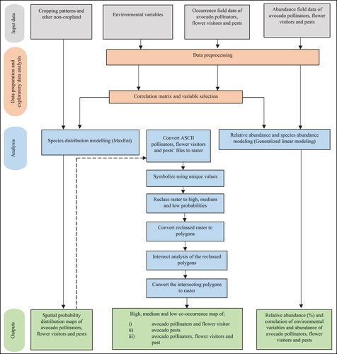
Figure 2 demonstrates the methodology used for species distribution modeling (SDM), co-occurrence analysis, and species abundance modeling (SAM). In summary: i) SDM involved using the MaxEnt model while integrating remotely sensed data of cropping patterns and non-croplands variables mapped in Aduvukha et al., (2021), avocado pollinators, flower visitors and pests occurrences sampled in NDVI informed avocado farms (Adan et al. 2021; Sagwe et al. 2021; Toukem et al. 2020) and environmental variables; ii) co-occurrence analysis involved intersection analysis of the outputs from the MaxEnt model; and iii) SAM involved utilizing the GLM, i.e. negative binomial distribution, to analyze the effect of the environmental variables on the abundance of the avocado pollinators, flower visitors, and pests. A detailed description of the datasets and analysis is presented herein.

Figure 2. Flow diagram of the approach adopted for the species distribution modelling, co-occurrence analysis, and species abundance modelling of avocado pollinators, flower visitors and pests. ASCII = American Standard Code for Information Interchange; MaxEnt = maximum entropy.

2.2.1. Earth observation remote-sensing data description and processing

2.2.1.1. Remote sensing datasets and field data collection

Remote sensing datasets of Sentinel-1 and Sentinel-2, as well as derived spectral indices and vegetation phenology and field data, were used in the mapping of cropping patterns and non-croplands, as described below (Aduvukha et al. 2021).

2.2.1.1.1. Sentinel-1 radar data

A total of 30 Sentinel-1 images were obtained from the European Space Agency (ESA) Copernicus data hub (ESA 2019) for all four seasons, i.e. hot dry (season 1, n = 5), long rainy (season 2, n = 9), cool dry (season 3, n = 8), and short rainy (season 4, n = 8) (Aduvukha et al. 2021). Sentinel-1 is a synthetic aperture radar sensor, providing images in the C-band frequencies continuously in all weather conditions, both day and night with a revisit period of 12 days (ESA 2019). The Sentinel-1 sensor acquires images in four modes, i.e.: stripmap (SM) (images small islands); interferometric wide swath (IW) (main acquisition over land); extra-wide swath (EW) (utilizes TOPSAR: Terrain Observation with Progressive Scans to acquire wider area data compared to IW); and wave (uses “leap frog” acquisition mode). Processing levels of the modes include Level-0, Level-1 (Single Look Complex-(SLC), ground range detected-(GRD)), and Level-2. In detail, Level-0 contains noise, orbit and altitude information, internal calibration and echo source packets; Level-1 SLC products are processed at natural pixel spacing and they preserve the phase information, while Level-1 GRD products are generated with less speckle and increased image quality, as well as containing the detected amplitude; and Level-2 contains geolocated geophysical products derived from Level-1 (ESA 2019). This study utilized the IW and Level 1 GRD products. Vertical transmit and vertical receive (VV) and vertical transmit and horizontal receive (VH) modes of dual polarization were utilized in Sentinel-1 images. The sensor image pre-processing was carried out using the Sentinel application platform (SNAP) toolbox and they included the application of the precise orbit file, thermal noise and image border, radiometric calibration, and speckle filtering (Filipponi 2019). In addition, the 90 m shuttle radar topography was bilinearly resampled to 10 m for terrain correction of the Sentinel-1 data. A subset composite image VV and VH image of each season was then obtained after stacking the individual processed images (Aduvukha et al. 2021).

2.2.1.1.2. Sentinel-2

Time-series (10 December 2017 to 15 December 2018) multi-sensor datasets from the freely available Sentinel-2 sensor and Sentinel-1 sensor were utilized in this study. Sentinel-2 comprises optical imagery of 13 multiple spectral bands, spanning across the visible, near-infrared, and short-wave infrared part of the spectrum, with resolutions ranging between 10 m, 20 m, and 60 m. It covers a horizontal distance of 290 km as it captures the Earth’s surface images (ESA 2019). A total of 128 images across four seasons were used, i.e. hot dry (season 1, n = 42), long rainy (season 2, n = 24), cool dry (season 3, n = 22) and short rainy (season 4, n = 40) (Aduvukha et al. 2021). Atmospheric correction (reducing the atmosphere’s effects of scattering and absorption on the reflectance values of images captured by satellite or aerial sensors) was carried out using the Sen2cor module in the SNAP toolbox (ESA 2019). Other preprocessing procedures performed in SNAP included cloud masking, resampling (20 m Sentinel-2 bands to 10 m, using the nearest-neighbor technique), layer stacking, mosaicking, and computation of the median pixel image for each season. The Sentinel-2 spectral bands used were bands 2, 3, 4, 5, 6, 7, 8a, 11, and 12 (Aduvukha et al. 2021).

2.2.1.1.3. Vegetation indices

Vegetation indices are used to describe various aspects of vegetation, including vegetation cover, vegetation health, and vegetation water content features, through using a combination of the spectral characteristics of more than one wavelength (Xue and Su 2017). Eight indices (Table 1) were derived from the composite seasonal images of Sentinel-2 imagery and used in this study (Aduvukha et al. 2021).

Table 1. Summary of the vegetation indices used in the mapping of cropping patterns and non-croplands, as adopted from Aduvukha et al. (2021).

No.	Index	Formula	Reference
1	Atmospherically resistant vegetation index-2 (ARVI2)	$-0.18+1.17\ast \left(\frac{\mathit{NIR}-\mathit{Red}}{\mathit{NIR}+\mathit{Red}}\right)$	(Kaufman and Tanre 1992)
2	Enhanced vegetation index (EVI)	$2.5\ast \frac{\mathit{NIR}-\mathit{Red}}{\mathit{NIR}+6\ast \mathit{Red}-7.5\ast \mathit{Blue}+1}$	(Ahamed et al. 2011)
3	Green normalized difference vegetation index (GNDVI)	$\frac{\mathit{NIR}-\mathit{Green}}{\mathit{NIR}+\mathit{Green}}$	(Gitelson, Kaufman, and Merzlyak 1996)
4	Modified soil adjusted vegetation index (MSAVI)	$\frac{\left(\mathit{NIR}-\mathit{Red}\right)\left(1+\mathit{L}\right)}{\mathit{NIR}+\mathit{Red}+\mathit{L}}$	(Qi et al. 1994)
5	Normalized difference vegetation index (NDVI)	$\frac{\mathit{NIR}-\mathit{Red}}{\mathit{NIR}+\mathit{Red}}$	(Tucker et al. 1979)
6	Normalized difference water index (NDWI)	$\frac{\mathit{NIR}-\mathit{SWIR}3}{\mathit{NIR}+\mathit{SWIR}3}$	(Gao 1996)
7	Soil adjusted vegetation index (SAVI)	$\left(\frac{\mathit{NIR}-\mathit{Red}}{\mathit{NIR}+\mathit{Red}+0.5}\right)\ast \left(1+0.5\right)$	(Huete 1988)
8	Two-band enhanced vegetation index (EVI2)	$2.5\ast \frac{\mathit{NIR}-\mathit{Red}}{\mathit{NIR}+2.4\ast \mathit{Red}+1}$	(Jiang et al. 2007)

Note: NIR= near-infrared band; L= 2*s*(NIR-Red) *(NIR-s* Red)/(NIR+Red), where s is the slope of the soil line from a plot of red versus near-infrared brightness values.

2.2.1.1.4. Phenological variable

Vegetation phenological variables were incorporated in this study, since they target the growth cycle of the vegetative components of the landscape (Kimball 2014). These variables (Araya 2017) (Table 2) were simulated from the multi-season NDVI images of Sentinel-2 using TIMESAT software (Jönsson and Eklundh 2004). Local functions were fit to the data points in the time-series NDVI curve data to analyze the phenological signals, which were then combined into a global model. Consequently, a smooth model function was employed to extract phenological variables for each season. A thresholding method, with a relative threshold of 0.3, was used to define the timings of the phenological events (Table 2) (Landman et al., unpublished work). A composite image for the vegetation phenological variables (n = 15) from each of the four seasons was created and used in the cropping pattern classification analysis (Table 2).

Table 2. Vegetation phenological variables that were used in mapping of cropping patterns and non-croplands, as adopted from Araya (2017) and Aduvukha et al. (2021).

No.	Phenological variable	Definition of the NDVI curve and physiological description
1	Onset_value	The NDVI value at the start of the growth (seedling growth stage)
2	Onset_time	The time when the growth onset is achieved
3	Max_value	The maximum NDVI value in the season
4	Max_time	The time when the Max_value is attained (anthesis growth stage)
5	Offset_value	The NDVI value at the end of the season
6	Offset_time	The time when growth offset is attained (senescence growth stage)
7	LengthGS	The length of the growing season
8	BeforeMaxT	The length of time between onset and Max_value
9	AfterMaxT	The length of time between Max_value and offset
10	GreenUpSlope	The rate of increase in NDVI value between onset and offset
11	BrownDownSlope	The rate of decrease in NDVI value between Max_value and offset
12	TINDVI	The area under the NDVI curve between onset and offset
13	TINDVIBeforeMax	The area under the NDVI curve between onset and Max_value
14	TINDVIAfterMax	The area under the NDVI curve between Max_value and offset
15	TINDVIAsymmetry	The difference between TINDVIBeforeMax and TINDVIAfterMax

2.2.1.1.5. Cropping pattern and non-croplands field data collection

Field data for cropping pattern and non-croplands were sampled from 12 December 2018 to 19 December 2018 (Aduvukha et al. 2021). The cropping patterns included monocrop maize, mixed crop maize, monocrop avocado, mixed crop avocado, monocrop coffee, monocrop tea and monocrop pineapple, while the non-croplands included areas of water, forest, shrubland, and built-up areas (Aduvukha et al. 2021). A stratified random sampling method was used to collect the ground truth field data as points (i.e. pixels) by using a mobile-based global positioning system (GPS), and GPS Essentials (GPS Essentials 2020) with a maximum allowable error of ±3 m. Furthermore, the collected field data points were set at a sampling distance of ≥20 m each to avoid spatial autocorrelation instances with respect to the 10 m resolution of Sentinel-2 imagery bands used. On-screen digitizing on high-resolution imagery provided by Google Earth imagery (Google Earth 2020) was then employed to convert the pixels of reference data to homogenous units (i.e. polygons) to be used for classification. Studies have shown that polygon-based training areas perform better than pixel-based training areas do (King’ori et al. 2023). A summary of the number of points and their corresponding pixels within the polygons of each class is shown in Aduvukha et al. (2021).

2.2.1.2 Cropping pattern and non-croplands classification

This included selecting the most important variables among the remote sensing dataset combinations (Table 3) and thereafter using a machine-learning algorithm for classification. Specifically, a guided regularized random forest (GRRF) algorithm was used to select important variables in each of the eight remotely sensed data combination scenarios (Table 3) (Aduvukha et al. 2021). The GRRF for selecting most important variables has been found to perform better than other methods, such as regularized random forest (RRF) and random forest (RF) algorithms, do (Deng and Runger 2013). The limitation of RF in selecting the most important variables lies in its susceptibility to select highly correlated variables, while RRF may select variables that are not robustly relevant (Deng and Runger 2013). On the other hand, the strength of GRRF in selecting the most robust variables lies in its facility to subject each feature to a penalty coefficient by altering the coefficient of importance of gamma (γ) value of 0 to 1, while maintaining the base coefficient of lambda (λ) value of 1 (Deng and Runger 2013). The importance of the variables was assessed using the mean decrease accuracy ranking method (Han, Guo, and Yu 2016). Further explanation of GRRF, RF and RRF in variable selection can be found in Deng and Runger (2013).

Table 3. The remote sensing datasets combination scenarios and number of variables for the classification of cropping patterns and non-croplands, as highlighted in Aduvukha et al. (2021).

Variable combination	Number of variables
Sentinel-2 bands only	40
Sentinel-2 bands and Sentinel-1	48
Sentinel-2 bands and vegetation indices	48
Sentinel-2 bands and vegetation phenology	55
Sentinel-2 bands, vegetation indices and Sentinel-1	56
Sentinel-2, vegetation indices and vegetation phenology	63
Sentinel-2, vegetation phenology and Sentinel-1	63
Sentinel-2, vegetation indices, vegetation phenology and Sentinel-1	71

Thereafter, a RF classification algorithm was used to delineate the different cropping patterns and non-croplands (Aduvukha et al. 2021). The RF algorithm was preferred to other supervised classification methods, such as maximum likelihood. This is because RF is non-parametric, i.e. it does not assume the data distribution but it learns first from the “seen” data and predicts the pattern of the “unseen” data (Breiman 2001; Wiener and Liaw 2002), thus reducing chances of overfitting. On the other hand, maximum likelihood assumes a normal distribution of the training data, hence high chances of overfitting the predictions (Sisodia, Tiwari, and Kumar 2014). Data were partitioned as 70% for training and 30% for testing (Aduvukha et al. 2021). The variable selection and cropping patterns and non-croplands classification were implemented in R software using the caret package (R Core Team 2019).

Consequently, the area under class method (Olofsson et al. 2013) was used to construct the confusion matrix for accuracy assessment to estimate the user’s accuracy (UA), producer’s accuracy (PA), overall accuracy (OA), and kappa coefficient (Aduvukha et al. 2021).

2.2.2. Pollinators, flower visitors, and pests field data collection

2.2.2.1. NDVI field characterization for sampling avocado farms

Time-series Sentinel-2 images of both dry and wet seasons accessed from the Google Earth Engine cloud computing platform were used (Gorelick et al. 2017). The seasons were determined from Climate Hazards Group InfraRed Precipitation with Station Data (CHIRPS) rainfall data (Adan et al. 2021). Ninety images for the dry season were obtained from 1 January 2018 to 28 February 2018, while 50 images for the wet season were obtained from 1 March 2018 to 31 March 2018. One hundred random points were generated within the study area, and a K-means clustering technique was used to categorize the extracted NDVI values into three levels, i.e. high, medium, and low (Table 4) (Adan et al. 2021).

Table 4. Normalized difference vegetation index (NDVI) of dry and wet seasons description and range, as described in Adan et al. (2021).

	NDVI range
NDVI intensity description	Dry season	Wet season
High	0.537–0.853	0.559–0.865
Medium	0.318–0.537	0.345–0.559
Low	<0.318	<0.345

The dry and wet season NDVI images were combined to provide a composite NDVI image (Adan et al. 2021). Using expert knowledge (observing texture, pattern, shade, tone, and color hue) (Li et al. 2020), the classification accuracy of the composite NDVI was assessed. An overall accuracy of 86.2% was attained, as detailed in Adan et al. (2021).

2.2.2.2. Sampling protocol for farms

The vegetation intensity classes of low, medium, and high obtained from NDVI as described in Section 2.2.2.1 were used as sampling strata, in which pollinator, flower visitor and pest data were collected in the study area. The sampling was carried out during the avocado peak flowering (26 August 2019–4 September 2019) and peak fruiting (27 January 2020–13 February 2020) seasons, respectively, in farm sizes of approximately 0.2–0.4 ha (Sagwe et al. 2021). Thirty-five farms were selected across the low, medium, and high NDVI regions, using a multi-stage sampling protocol, as detailed in Adan et al. (2021). In summary, the avocado farms selection protocol in each stratum included: (1) minimal number of avocado trees per farm at seven; (2) socio-economic data on farmers’ willingness-to-pay for IPPM technologies (IPM only where biological treatment of pests was introduced, pollinators only (P) where managed bees were introduced, IPPM where both managed bees and biological treatment of pests were introduced, and control where neither treatments of pests nor managed bees were introduced); and (3) setting specific distances among avocado farms with the different IPPM technologies. The specific distances between farms with the different technologies were as follows (i) IPPM and P were at least 1.5–3.0 km separate from each other, (ii) IPM and control were at least 0.5 km away from each other, and (iii) IPPM or P were at least 3.5 km away from either IPM or control sites (Adan et al. 2021). The implementation of the different IPPM technologies was assessed in a separate study by Toukem et al. (2022) to establish the effect of the inclusion of pollinators in pest management of crops such as avocado.

2.2.2.3. Avocado pollinator, flower visitor, and pest occurrence and abundance data

For purposes of this study, flower-visiting insects that are good at pollinating avocado crops were defined as “pollinators,” while those flower-visiting insects that are poor at pollinating avocado crops were called “flower visitors” (Sagwe et al. 2022). Furthermore, in this study, “occurrences” were defined as geolocated instances of the observed pollinator, flower visitor, or pest, while “abundance” was defined as the relative number (count) of a pollinator, flower visitor, or pest trapped per unit area of the farm size. Therefore, for avocado pollinators and flower visitors, three avocado trees, spaced 20 m apart within each of the selected farms, were randomly selected, and each of the three avocado trees was observed for 5 min from 0800 to 1700 h (Greenwich Mean Time: GMT + 3). The pollinators and/or flower visitors were captured using sweep nets (white in color) and were forthwith preserved in 70% ethanol (Sagwe et al. 2022). The sampled pollinators and flower visitors were identified by Robert Copeland, icipe, Nairobi, Kenya, and categorized into four groups: (1) A. mellifera (order Hymenoptera), (2) Hymenoptera excluding A. mellifera (order Hymenoptera), (3) Syrphidae (order Diptera) and (4) Calliphoridae (order Diptera). Other categories of pollinators or flower visitors were also sampled, but were of very low count, and thus were not included in this study.

Regarding avocado pests, traps for the specific pests were set on two separate avocado trees at a distance of ≥20 m apart in each of the selected farms (Toukem et al. 2020). Lynfield traps (icipe, Nairobi, Kenya) with para-pheromone methyl eugenol (River Bioscience, Addo, South Africa) were used to trap B. dorsalis, while T. leucotreta were trapped using white delta-shaped traps, lured with the relevant sex pheromone (Kenya Biologics, Nairobi, Kenya). Insects from the Lynfield traps were kept in 70% ethanol for preservation, while sheets with trapped insects from the white delta-shaped traps were enclosed in a polythene sheet before analysis in the laboratory, as detailed in Toukem et al. (2020). The pests were subsequently identified by Robert Copeland, icipe, Nairobi, Kenya. On the other hand, the abundance of the avocado pests was collected after 2 weeks within the sampling period only on 17 farms that were set as control treatments out of the total 35 selected farms, since the other 18 farms were put on other IPPM treatments before sampling the abundance of pests.

A mobile-based GPS application, i.e. GPS Essentials (Schollmeyer Software Engineering, Munich, Germany), was used to geolocate the specific trees within each avocado farm where pollinators, flower visitors, and pests were sampled.

2.2.3. Predictor variables

2.2.3.1. Environmental predictor variables and preprocessing

The most influential environmental variables that affect the distribution and abundance of avocado pollinators, flower visitors, and pests were used as predictor variables in the modeling experiments (Kjøhl, Nielsen, and Stenseth 2011; Odanga et al. 2018). These were average temperature, precipitation, solar radiation, wind speed, morning relative humidity, afternoon relative humidity, and elevation (Table 5). Slope, hillshade, and aspect were derived from elevation. In addition, the variable “cropping patterns,” which were derived from Aduvukha et al. (2021), were also included as comprising a predictor variable. These cropping patterns were monocrop tea, mixed crop avocado, mixed crop maize, monocrop avocado, monocrop coffee, monocrop maize, and monocrop pineapple and non-croplands. For the environmental variables, long-term mean average values of July, August, September, and October, estimated from 1961 to 1990 and 1970 to 2000 (Kriticos et al. 2012; Fick and Hijmans 2017), were used in predicting pollinator and flower visitor spatial distribution probability, as they coincide with the pre-peak, during and post-peak flowering seasons of avocado in the study area. This period also coincided with the pollinator and flower visitor field data collection. For pest spatial distribution probability modeling, long-term mean average values of the environmental variables, estimated from 1961 to 1990 and 1970 to 2000 for December, January, February, and March, were used. This matched with the avocado pre-peak, during and post-peak fruiting season in Kenya, during which the pests were sampled.

Table 5. Predictor variables used in spatial distribution and abundance analysis of avocado pollinators, flower visitors, and pests.

Variable	Unit	Resolution	Year	Source
Average temperature	°C	1 km	1970–2000	(Fick and Hijmans 2017)
Precipitation	mm	1 km	1970–2000	(Fick and Hijmans 2017)
Solar radiation	kJ m^−2 day^−1	1 km	1970–2000	(Fick and Hijmans 2017)
Wind speed	m s^−1	1 km	1970–2000	(Fick and Hijmans 2017)
Relative humidity (morning)	%	1 km	1961 - 1990	(Kriticos et al. 2012)
Relative humidity (afternoon)	%	1 km	1961-1990	(Kriticos et al. 2012)
Elevation	m	1 km		(Fick and Hijmans 2017)
Slope	%rise	30 m	n/a	Derived from elevation
Hillshade	n/a	30 m	n/a	Derived from elevation
Aspect	degrees	30 m	n/a	Derived from elevation
Cropping pattern	n/a	10 m	2018	Aduvukha et al. (2021)

n/a=not applicable.

The bilinear interpolation method was used to resample the environmental predictor variables to 10 m × 10 m pixel size and then clipped to the size of the study area to be harmonized with the cropping pattern predictor variable that was developed by Aduvukha et al. (2021).

2.2.3.2. Predictor variable selection

The variance inflation factor (VIF) was used to determine the most uncorrelated predictor variables to reduce multicollinearity (Robinson and Schumacker 2009). A VIF threshold of ≥10 was set as an indicator of multicollinearity and redundancy in the predictor variables (Pradhan 2016) (Table 6). The total number of predictor variables subjected to VIF were n = 11 (Table 1) for the pollinators, flower visitors, and pests, with seven predictor variables being retained for pollinators and flower visitors, while eight predictor variables were retained for the pests (Table 6). However, some of the key predictor variables, such as temperature that is known to influence the distribution of pollinators, flower visitors, and pests, were suggested for exclusion by the VIF test. However, some of these predictor variables were retained, for instance, average temperature, based on their biological relevance to avocado pollinators and flower visitors (average temperature with VIF of 135.99) and pests (average temperature with VIF of 70.71) distribution and abundance (EFSA 2011; Pradhan 2016).

Table 6. Variables selected after performing multicollinearity analysis using the variance inflation factor (VIF) of a minimum of 10 for avocado pollinators, flower visitors, and pests.

	Variable	VIF <10
Avocado pollinators/Flower visitors	aspect	1.11
	cropping pattern	1.01
	hillshade	1.18
	precipitation	7.53
	morning relative humidity	5.52
	slope	1.34
	wind speed	3.43
Avocado pest	aspect	1.10
	cropping pattern	1.12
	hillshade	1.16
	precipitation	4.07
	afternoon relative humidity	2.72
	slope	1.24
	solar radiation	8.69
	wind speed	4.14

2.2.4. Species distribution modelling

2.2.4.1. Model settings

Before applying the SDMs to predict the spatial distribution probability of avocado pollinators, flower visitors, and pests, the geolocations of avocado pollinators, flower visitors, and pest observations were reprojected to the Universal Transverse Mercator (UTM) coordinate system, zone 37 south (Snyder 1987). This was done to ensure compatibility with the coordinate system of the predictor environmental variables.

The MaxEnt model, Version 3.4.1 (Phillips and Dudík 2008), was used to predict potentially suitable areas of avocado pollinators, flower visitors, and pest distributions. The model settings of the MaxEnt were majorly influenced by the number of occurrence points for each of the avocado pollinators, flower visitors, and pests (Phillips and Dudík 2008). Consequently, this influenced the MaxEnt feature types in modeling the avocado pollinators, flower visitors, and pests (Table S1 in Supplementary). Outliers were eliminated using a “ten percentile” training presence criterion, which declares the 10% most extreme presence observation as absent (Cord et al. 2014). Additionally, a regularization multiplier of two was employed to ensure a less localized prediction (Radosavljevic, Anderson, and Araújo 2014). Moreover, to ascertain a robust MaxEnt model, the replicate runs were set to 10 (Makori et al. 2017). Cross-validation replication type was used for A. mellifera, Syrphidae, Calliphoridae, B. dorsalis and T. leucotreta because of its robustness (Kohavi 1995), while a bootstrap replication type for Hymenoptera excluding A. mellifera was used because of the small sample size (Merow, Smith, and Silander 2013). A sensitivity analysis of the variable contribution to the model was conducted using a jackknife test. The jackknife test assesses how each variable affects the performance of the model by determining changes in the accuracy of the model as it systematically eliminates one variable at a time. The critical variables for predictions are identified by comparing how the model performs, with and without each variable (Phillips and Dudík 2008).

2.2.4.2. Model performance assessment

Model performance of the prediction of spatial distribution probability for the occurrence of avocado pollinators, flower visitors, and pests was assessed using the receiver operating characteristic (ROC)‘s threshold-independent area under the curve (AUC) (Merow, Smith, and Silander 2013). The AUC informs the probability of whether presence (sensitivity) in comparison to absence (specificity) was ordered correctly by the model. The values of AUC range from 0 (no possibility of occurrence) to 1 (highest possibility of occurrence), with values greater than 0.7 being regarded as acceptable for predicting spatial distribution probability for the species (Araújo et al. 2005).

2.2.4.3. Co-occurrence spatial distribution of avocado pollinators, flower visitors, and pests

Potential co-occurrence analysis of the sampled pollinators, flower visitors, and pests was carried out using the spatial distribution probability outputs generated from MaxEnt. The MaxEnt outputs were in the American Standard Code for Information Interchange (ASCII) file format, which were first converted to the raster image file format (tiff) and assigned three unique values: low, medium, or high. The tiff files were reclassified to low (0.01–0.35), medium (0.36–0.69), and high (0.70–0.99) classes. These classes represented the cluster thresholds of co-occurrence spatial distribution probability of the pollinators, flower visitors, and pests, from the co-occurrence analysis. Each of the tiff files was converted to a vector polygon file to perform an intersect analysis among the respective classes represented by the respective polygons. This was done to assess areas of similarity between the pollinators and flower visitors (only pollinators and flower visitors) and pests (only pests) and also to compare the co-occurrence with the occurrence of all pollinators, flower visitors, and pests. Intersecting polygons were converted to raster data, resulting in the delineation of co-occurrence spatial distribution probabilities of all the pollinators and flower visitors, all the pests, and all the combined pollinators, flower visitors, and pests.

2.2.5. Species abundance modelling

A generalized linear model (GLM) was implemented in R software, Version 3.6.1 (R Core Team 2019) to infer the relationship between the abundance of the avocado pollinators, flower visitors, and pests, and the selected environmental predictor variables. Specifically, the negative binomial distribution in GLM, which accommodates overdispersion of integer counts data, was used (Lindén and Mäntyniemi 2011). The coefficient estimates of all the environmental predictor variables and their significance level (p ≤ 0.05) were analyzed to assess their relationships with the abundance of avocado pollinators, flower visitors, and pests. Hymenoptera species excluding A. mellifera pollinators were not included in this analysis because of their very low counts (n = 8).

3. Results

3.1. Cropping pattern and non-croplands

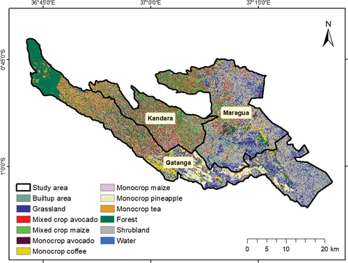
The best-performing classification scenario (OA = 94.33% and kappa = 0.93) (Table S2 in Supplementary), i.e. Sentinel-2 bands, vegetation indices and Sentinel-1 combination, was used in the spatial modeling of the avocado pollinators, flower visitors and pests (Aduvukha et al. 2021). The mapped cropping patterns were monocrop avocado, mixed crop avocado, monocrop maize, mixed crop maize, monocrop coffee, monocrop tea, and monocrop pineapple while the non-croplands were comprised of built-up area, grassland, forest, shrubland, and water (Figure 3).

Figure 3. Map of cropping pattern and non-croplands in Kandara, Maragua and Gatanga sub-Counties, Murang’a County, Kenya (Aduvukha et al. 2021).

3.2. Species distribution modelling

3.2.1. Maximum entropy (MaxEnt) model performance

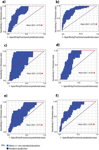
All the MaxEnt models used for predicting the spatial distribution probability of all the studied avocado pollinators (A. mellifera, Hymenoptera excluding A. mellifera and Syrphidae), flower visitors (Calliphoridae) and pests (B. dorsalis and T. leucotreta) demonstrated a good prediction performance within an AUC of 0.70–0.83 (Figure 4).

Figure 4. Mean area under the curve (AUC) to two decimal places for predicting spatial distribution probability of (a) Apis mellifera, (b) Hymenoptera excluding A. mellifera, (c) Syrphidae (d) Calliphoridae (e) Bactrocera dorsalis, and (f) Thaumatotibia leucotreta.

3.2.2. Predictor variable contribution

The first three ranked variables for the prediction of pollinator distribution were wind speed (38.10%), precipitation (28.60%) and cropping patterns (26.60%) for A. mellifera; cropping pattern (39.40%), aspect (25.00%), and wind speed (18.70%) for Hymenoptera excluding A. mellifera; cropping pattern (57.80%), precipitation (33.70%), and wind speed (8.00%) for Syrphidae; and precipitation (45.50%), wind speed (41.70%), and cropping pattern (9.5%) for Calliphoridae (Table 7). The first three ranked variables for avocado pest distribution were cropping pattern (47.00%), average temperature (42.90%) and wind speed (2.60%) for B. dorsalis; and cropping pattern (44.30%), slope (28.50%) and average temperature (19.80%) for T. leucotreta (Table 8). Based on the jackknife tests performed on the MaxEnt model, the relative variable importance of the cropping pattern and environmental variables showed varied contributions on the ecological niche (EN) models (Figure S1 in Supplementary).

Table 7. Contribution (%) of predictor variables to Apis mellifera, Hymenoptera excluding A. mellifera, Syrphidae, and Calliphoridae spatial distribution probability from maximum entropy (MaxEnt) models using the jackknife test.

Variable	Apis mellifera	Hymenoptera excluding A. mellifera	Syrphidae	Calliphoridae
Cropping pattern	26.60	39.40	57.80	9.50
Aspect	1.60	25.00	0.30	1.80
Hillshade	0.20	6.10	0.00	0.10
Precipitation	28.60	7.20	33.70	45.50
Morning relative humidity	4.40	0.10	0.10	0.30
Slope	0.50	1.40	0.00	1.10
Average temperature	0.00	2.00	0.00	0.00
Wind speed	38.10	18.70	8.00	41.70

Table 8. Contribution (%) of predictor variables to Bactrocera dorsalis and Thaumatotibia leucotreta spatial distribution probability from maximum entropy (MaxEnt) models using the jackknife test.

Variable	Bactrocera dorsalis	Thaumatotibia leucotreta
Cropping pattern	47.00	44.30
Aspect	1.50	0.70
Hillshade	0.00	1.10
Precipitation	1.90	3.80
Afternoon relative humidity	1.50	0.30
Slope	1.10	28.50
Solar radiation	1.60	0.40
Average temperature	42.90	19.80
Wind speed	2.60	1.00

3.2.3. Spatial distribution probability of avocado pollinators, flower visitors, and pests

The MaxEnt model for avocado pollinators (A. mellifera and Syrphidae) and avocado flower visitors (Calliphoridae) predicted a medium to a high spatial probability distribution in Kandara sub-County, and a low to a high spatial probability distribution in Maragua and Gatanga sub-Counties (Figure 5a–c and d). The majority of Kandara and portions of Maragua and Gatanga sub-Counties experienced the highest spatial distribution probability score of >0.9 for the presence of A. mellifera and Syrphidae pollinators, and Calliphoridae flower visitors. The MaxEnt model for Hymenoptera excluding A. mellifera pollinators (Figure 5b) also showed a low to a high spatial probability distribution score in the three sub-Counties.

Figure 5. Spatial distribution probability of avocado pollinators (a) Apis mellifera, (b) hymenoptera excluding Apis mellifera, and (c) Syrphidae; avocado flower visitors (d) Calliphoridae and avocado pests (e) Bactrocera dorsalis (f) Thaumatotibia leucotreta predicted using the maximum entropy (MaxEnt) model. The dark blue color indicates a low spatial distribution probability, while the red color represents a high spatial distribution probability. The resolution of the maps is 10 m in relation to spatial resolution of the cropping pattern variable.

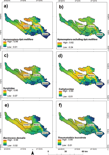
The MaxEnt model predicted high avocado pest spatial probability distribution scores (≥0.9) in the central and western sides of Maragua and Kandara sub-Counties, and low to high scores in Gatanga sub-County. A low distribution score was observed in the eastern side of Maragua and Gatanga sub-Counties for B. dorsalis and T. leucotreta (Figure 5e, f respectively).

3.2.4. Co-occurrence spatial distribution probability of avocado pollinators, flower visitors, and pests

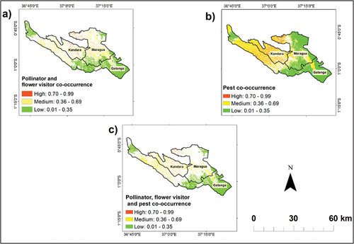
The avocado pollinator and flower visitor co-occurrence analysis showed a low to high probability of co-occurrence in the three studied sub-Counties, with the majority of Kandara showing a medium to high probability of pollinator and flower visitor co-occurrence (Figure 6a). Further, avocado pest co-occurrence analysis showed a medium to high probability of co-occurrence in Kandara, while a low to a high probability of co-occurrence was present in Gatanga and Maragua (Figure 6b). On the other hand, the combined co-occurrence analysis of avocado pollinators, flower visitors, and pests showed a medium to a high probability of co-occurrence in Kandara and a low to a high probability of co-occurrence in Maragua and Gatanga. (Figure 6c). The accuracy of the co-occurrence analysis (Figure 6) is taken to be similar to those of Figure 5 (SDM) since the inputs used are derived from Figure 5.

Figure 6. Spatial distribution probability of co-occurrence of (a) avocado pollinators and flower visitors (b) avocado pests and (c) avocado pollinators, flower visitors and pests. The light green color indicates a low probability of co-occurrence spatial distribution, while the yellow and the red colors represent a medium and a high probability of co-occurrence, respectively. The resolution of the maps is 10 m in relation to spatial resolution of the cropping pattern variable.

3.3. Species abundance modelling

3.3.1. Avocado pollinator, flower visitor, and pest abundance

The relative abundance of the avocado pollinators and flower visitors showed that A. mellifera was relatively more abundant (80.84%) than Calliphoridae (10.05%) and Syrphidae (9.11%). Among the avocado pests, the relative abundance of B. dorsalis (96.62%) was higher than that of T. leucotreta (3.38%) (Table 9). Distribution of the abundance avocado pollinators, flower visitors, and pests per their respective farms are summarized in Table S3 in Supplementary.

Table 9. The abundance (n) and relative abundance (%) of avocado pollinators, flower visitors, and pests.

Avocado pollinators, flower visitors and pests	Abundance (n)	Relative abundance (%)
Apis mellifera	503	80.48
Syrphidae	58	9.28
Calliphoridae	64	10.24
Total	625	–
Bactrocera dorsalis	25,433	96.62
Thaumatotibia leucotreta	889	3.38
Total	26,322	–

3.3.2. Generalized linear model

Abundance of A. mellifera had a positive relationship with precipitation, slope, and wind speed, but a negative relationship with aspect, hillshade, morning relative humidity, and average temperature (Table 10). Furthermore, the results showed that the abundance of Syrphidae pollinators had a positive relationship with aspect, precipitation, morning relative humidity, slope, average temperature, and wind speed, but a negative relationship with hillshade, while the abundance of Calliphoridae flower visitors had a positive relationship with aspect, hillshade, and wind speed, but a negative relationship with precipitation, morning relative humidity, slope, and average temperature. No variable was significant (p ≤ 0.05) for pollinators and flower visitors.

Table 10. Summary of the relationship between the environmental variables and the abundance of avocado pollinators, flower visitors, and pests depicting the regression coefficient estimates and p-value (p ≤ 0.05).

Avocado pollinators, flower visitors and pests	Environmental variables	Estimate	p-value
Apis mellifera	(Intercept)	8.53	0.69
	aspect	−0.00	0.34
	hillshade	−0.01	0.24
	slope	0.03	0.19
	precipitation	0.01	0.60
	average temperature	−0.23	0.61
	morning relative humidity	−0.14	0.58
	wind speed	3.74	0.17
Syrphidae	(Intercept)	−32.40	0.33
	aspect	0.00	0.27
	hillshade	−0.00	0.71
	slope	0.02	0.49
	precipitation	0.02	0.92
	average temperature	0.48	0.49
	morning relative humidity	0.22	0.56
	wind speed	4.46	0.13
Calliphoridae	(Intercept)	5.31	0.80
	aspect	0.00	0.75
	hillshade	0.01	0.18
	slope	−0.24	0.40
	precipitation	−0.01	0.76
	average temperature	−0.32	0.53
	morning relative humidity	−0.13	0.59
	wind speed	3.66	0.31
Bactrocera dorsalis	(Intercept)	73.56	0.025*
	aspect	−0.00	0.00*
	precipitation	−0.38	<0.001*
	hillshade	0.04	4.15e-08*
	slope	0.04	0.12
	afternoon relative humidity	0.08	0.48
	average temperature	1.16	0.19
	wind speed	−1.99	0.20
	solar radiation	−0.00	0.22
Thaumatotibia leucotreta	(Intercept)	127	0.00**
	aspect	5.47e-04	0.62
	precipitation	−8.11e-02	0.43
	hillshade	−5.97e-04	0.95
	slope	−5.07e-02	0.13
	afternoon relative humidity	3.48e-02	0.83
	average temperature	1.29e+00	0.24
	wind speed	1.74e+00	0.34
	solar radiation	−7.68e-03	0.03*

*Significant variables (p ≤ 0.05).

Regarding the avocado pests, the abundance of B. dorsalis had a positive relationship with hillshade, slope, average temperature, and afternoon relative humidity, but a negative relationship with aspect, precipitation, wind speed, and solar radiation (Table 10). However, only the relationship between the abundance of B. dorsalis with aspect, precipitation, and hillshade was statistically significant (p ≤ 0.05). Thaumatotibia leucotreta abundance showed a positive relationship with aspect, afternoon relative humidity, average temperature and wind speed, but a negative relationship with precipitation, hillshade, slope and solar radiation, with only solar radiation being statistically significant (p ≤ 0.05).

4. Discussion

This study predicted the spatial distribution of avocado pollinators, flower visitors, and pests in Murang’a County, Kenya using accurate remotely sensed cropping patterns (OA 94.33% and kappa 0.83), environmental factors as predictor variables, and the MaxEnt ecological niche modeling approach. In addition, the study revealed the co-occurrence spatial distribution probability of the studied avocado pollinators, flower visitors, and pests. Furthermore, the study also examined the relationship between the abundance of avocado pollinators, flower visitors, and pests with environmental variables by using a GLM model.

4.1. Species distribution modelling

The study identified highly suitable habitats for each of the avocado pollinators, flower visitors, and pests in the northern and central parts of Kandara, the north-western part of Gatanga, and the south-eastern part of Maragua. These regions are characterized by conducive climatic conditions for avocado farming and thus demonstrated the importance of the LULC variable in predicting pollinator, flower visitor, and pest habitats or invasive plant species (Sittaro, Hutengs, and Vohland 2023; Tonnang et al. 2017). In terms of the influence of environmental variables on the distribution of the avocado pollinators and flower visitors, the present study suggests that the distribution of the pollinators and flower visitors had a negative correlation with high wind speed (>2.5 ms⁻¹, Figure S2 in Supplementary). There is a likelihood of increased resistance of the flight of A. mellifera and Syrphidae pollinators with high wind speed, especially in the opposite direction (not measured in this study). This may cause a reduced flower visitation rate, consequently reducing their distribution (Hennessy et al. 2020). Wind speed has also been observed to contribute to an increased rate of cooling of some Diptera pollinators (Inouye et al. 2015). The high precipitation (>40 mm, Figure S2 in Supplementary) reported in this study area may be unsuitable for the distribution of A. mellifera and Syrphidae pollinators, and Calliphoridae flower visitors. Previous studies have highlighted how high rainfall negatively affects the foraging and flight activities of A. mellifera pollinators, which may have resulted in their lower occurrence (González et al. 2009).

Average temperature can positively affect the survival, development, and reproduction of crop insect pests, thus affecting their distribution (Zingore et al. 2020). Studies have indicated that T. leucotreta survives and propagates successfully in a temperature range between 16°C and 30°C (Jager and Marthalise 2013). Likewise, Choi et al. (2020) reported that the same temperature range positively influenced the fertility of B. dorsalis in the laying of eggs. Moreover, slope (>0%, <10%, Figure S2 in Supplementary), which is a derivative of elevation, positively influenced the spatial distribution probability of both B. dorsalis and T. leucotreta. This result corroborates Odanga et al. (2018) who found that B. dorsalis distribution increased as elevation decreased, since B. dorsalis is a lowland pest. On the other hand, this study demonstrated that wind speed negatively affected the distribution of B. dorsalis, which implies that regions with high wind speed (≥3.2 ms⁻¹, Figure S2 in Supplementary) would, for instance, negatively affect the flight of B. dorsalis, hence affecting their distribution (Susanto et al. 2022).

Co-occurrence analysis revealed that a large area of Kandara exhibited medium to high-probability co-occurrence of the studied pollinators, flower visitors, and pests individually and combined. Sharing of the ecological niches between the studied pollinators, flower visitors, and pests may cause the competition for resources, especially by the dominant pollinator and pest thus affecting the populations of other pollinators, flower visitors, and pests (Mahmoud et al. 2020). Nonetheless, there is a possibility of “minor” pollinators, flower visitors and pests to adapt to new ecological niches for their survival (Hassani et al. 2022).

4.2. Species abundance and generalized linear modelling

In this study, A. mellifera (order Hymenoptera) was more abundant, compared with Syrphidae (order Diptera) pollinators and Calliphoridae flower visitors (order Diptera). Earlier studies have shown that A. mellifera has been observed to be the most abundant pollinator in fruit crop systems including avocado (Kjøhl, Nielsen, and Stenseth 2011), although A. mellifera is often a managed species. The B. dorsalis avocado pest was more abundant than T. leucotreta, presumably owing to the presence of other suitable host plants, e.g. mangos, which were also in their fruiting season during the time of the field data collection.

The relationship between average temperature and morning relative humidity was negative to the abundance of A. mellifera since these pollinators prefer to start most of their activity at lower temperatures (12°C to 13°C) and because moderate morning relative humidity provides warm and cooler conditions that also increase their activity (Nikolova et al. 2016). On the other hand, wind speed showed a positive relationship with the abundance of A. mellifera in this present study, but Hennessy et al. (2020) have reported that an increase in wind speed increased the resistance of the flight of bees, thereby causing fewer flowers to be visited. The negative relationship of abundance of A. mellifera with the aspect and hillshade, which are both derivatives of elevation, can be explained by the species-area relationship, whereby an increase in elevation may also affect the air temperature, which tends to be cooler than the minimum temperature for A. mellifera activity (Lefebvre et al. 2018). On the other hand, precipitation showed a positive relationship with the abundance of A. mellifera, although high precipitation may cause mechanical difficulty in the flight of A. mellifera, thereby affecting the visitation of these pollinators – hence lower count observations (Lawson and Rands 2019). Surprisingly, no environmental variable was significant to the abundance of A. mellifera supposedly because of the near indistinctive differences in the abundance counts among the different observed farms.

The positive relationship between the abundance of B. dorsalis and T. leucotreta and average temperature and afternoon relative humidity can be explained by the importance of temperature and moisture in improving pest egg formation (Potting and van der Straten 2010; Rashmi et al. 2020). Interestingly in this study, the abundance of B. dorsalis is shown to be positively correlated with hillshade and aspect, which are derivatives of elevation. This is contrary to Odanga et al. (2018), who found that B. dorsalis populations are negatively correlated with an increase in elevation. On the other hand, slope, and hillshade, which are derivatives of elevation, showed a negative relationship with the abundance of T. leucotreta. Odanga et al. (2018) demonstrated the fact that these pests exhibited no distinguishing characteristics across different altitudinal ranges owing to their wider tolerance to temperature ranges, which are also affected by altitude.

The negative relationship between the abundance of B. dorsalis and T. leucotreta and precipitation is presumably caused by the inhibition of survival of the larva-pupal stage of the pest, which is inhibited when soil moisture is beyond the field capacity, while T. leucotreta is more present in warmer humid areas (Montoya, Flores, and Toledo 2008; Potting and van der Straten 2010). Wind speed had a negative relationship with the abundance of B. dorsalis in the present study, in that an increase in the speed of wind, especially in the opposing direction, can cause flight resistance of the pest, thus affecting their flight to the targeted area (Susanto et al. 2022). On the contrary, Verghese et al. (2006) found that wind speed had a positive relationship with the abundance of B. dorsalis, as the wind can also be a medium of dispersing the metathyl food lure for B. dorsalis, hence attracting them, and subsequently increasing the abundance of B. dorsalis catches. An increase in solar radiation causes an increase in temperature, whereby extremely high temperatures negatively affect B. dorsalis (Shrestha, Thapa, and Gautam 2019). The relationship between the abundance of B. dorsalis and precipitation, aspect and hillshade was significant (p ≤ 0.05), supposedly because of the contribution of these variables to temperature variations.

The positive relationship between wind speed and the abundance of T. leucotreta could have influenced more numbers of T. leucotreta to be trapped, since the wind may aid the swinging of the traps for an increased number of T. leucotreta captures (Moore 2019). Presumably, the significance (p ≤ 0.05) of the relationship of the abundance of T. leucotreta with solar radiation demonstrated in the results was caused by the direct temperature effect on the degree of moisture, i.e. relative humidity, thus directly affecting the abundance of T. leucotreta (Potting and van der Straten 2010).

The relationships between the abundance of Syrphidae and Calliphoridae and the environmental variables observed in this study may be inconclusive. This is because their observed counts in the sampled farms did not exhibit population densities that varied significantly for proper interpretation. A longer sampling period could provide an opportunity to sample increased species abundance (Mandela et al. 2018).

This study summarized Hymenoptera excluding A. mellifera, Syrphidae and Calliphoridae into larger groups such as families to increase the sample size suitable for the spatial distribution modeling. This may result in broadening the ecological niches of species in the specific orders and families, and so fail to account for species-specific ecological niches. However, the findings can be useful in deducing the general behavior of the respective pollinators and flower visitors, in comparison with other pollinators, such as A. mellifera of the Apidae family.

5. Conclusions

This study revealed the possibility of combining accurate remotely sensed variables of cropping patterns and environmental variables in investigating the spatial distribution and abundance of the avocado pollinators, flower visitors, and pests (AUC > 0.70). Specifically, this study revealed that the studied pollinators, flower visitors, and pests had a medium to high probability of occurrence in Kandara and some parts of Maragua. Gatanga had a varied probability of their occurrence, from low to high. This study also highlighted the dominance of A. mellifera avocado pollinators and B. dorsalis as avocado pests. Moreover, the co-occurrence analysis of the avocado pollinators, flower visitors and pests also demonstrated the potential regions of their high, medium, and low simultaneous occurrences. This is crucial in providing key information necessary for the decision-makers and farmers in the implementation of IPPM techniques at a landscape scale. Future studies could look into the spatial modeling of these insects, during off-peak and peak flowering and fruiting seasons, in regions of similar agroecological zone settings. This would help to capture the diversity of the avocado insects and compare the most influential variables in the abundance of these insects in the different seasons. Consequently, this would further aid in the development of recommender systems for intelligent implementation of sustainable development efforts, such as IPPM.

Acknowledgments

We thank Rose Sagwe and Toukem Nadia for their assistance in collecting the occurrence and abundance data of avocado pollinators, flower visitors, and pests. Much appreciation also goes to the avocado farmers in Murang’a County Kenya, for their cooperation and for providing us with the information needed for this project.

Disclosure statement

No potential conflict of interest was reported by the author(s).

Supplementary material

Supplemental data for this article can be accessed online at https://doi.org/10.1080/15481603.2024.2347068

Data availability statement

All datasets presented in this study are included in the article and can be made available by the authors upon request.

Additional information

Funding

This work received financial support from the German Federal Ministry for Economic Cooperation and Development (BMZ), commissioned and administered through the Deutsche Gesellschaft für Internationale Zusammenarbeit (GIZ) Fund for International Agricultural Research (FIA), grant number 17.7860.4–001; the Norwegian Agency for Development Cooperation, the Section for Research, Innovation, and Higher Education, grant number RAF-3058 KEN-18/0005; the Swedish International Development Cooperation Agency (Sida); the Swiss Agency for Development and Cooperation (SDC); the Australian Centre for International Agricultural Research (ACIAR); the Norwegian Agency for Development Cooperation (Norad); the German Federal Ministry for Economic Cooperation and Development (BMZ); and the Government of the Republic of Kenya. The views expressed herein do not necessarily reflect the official opinion of the donors.

References

- Adan, M., E. M. Abdel-Rahman, S. Gachoki, B. W. Muriithi, H. M. G. Lattorff, V. Kerubo, T. Landmann, S. A. Mohamed, H. E. Z. Tonnang, and T. Dubois. 2021. “Use of Earth Observation Satellite Data to Guide the Implementation of Integrated Pest and Pollinator Management (IPPM) Technologies in an Avocado Production System.” Remote Sensing Applications: Society & Environment 23:100566. https://doi.org/10.1016/j.rsase.2021.100566.
- Aduvukha, G. R., E. M. Abdel-Rahman, A. W. Sichangi, G. O. Makokha, T. Landmann, B. T. Mudereri, H. E. Z. Tonnang, and T. Dubois. 2021. “Cropping Pattern Mapping in an Agro-Natural Heterogeneous Landscape Using Sentinel-2 and Sentinel-1 Satellite Datasets.” Agriculture 11 (6): 530–22. https://doi.org/10.3390/agriculture11060530.
- Ahamed, T., L. Tian, Y. Zhang, and K. C. Ting. 2011. “A Review of Remote Sensing Methods for Biomass Feedstock Production.” Biomass and Bioenergy 35 (7): 2455–2469. https://doi.org/10.1016/j.biombioe.2011.02.028.
- Araújo, M. B., R. G. Pearson, W. Thuiller, and M. Erhard. 2005. “Validation of Species–Climate Impact Models Under Climate Change.” Global Change Biology 11 (9): 1504–1513. https://doi.org/10.1111/j.1365-2486.2005.01000.x.
- Araya, S. 2017. Multi-Temporal Remote Sensing for the Estimation of Plant Available Water-Holding Capacity of Soil. Phd Thesis, University of Adelaide, Adelaide, Australia.
- Biddinger, D., and E. Rajotte. 2015. “Integrated Pest and Pollinator Management – Adding a New Dimension to an Accepted Paradigm.” Current Opinion in Insect Science 10:204–209. https://doi.org/10.1016/j.cois.2015.05.012.
- Breiman, L. 2001. “Random Forests.” Machine Learning 45 (1): 5–32. https://doi.org/10.1023/A:1010933404324.
- Choi, K. S., A. C. Samayoa, S.-Y. Hwang, Y.-B. Huang, J. J. Ahn, and J. J. Hull. 2020. “Thermal Effect on the Fecundity and Longevity of Bactrocera Dorsalis Adults and Their Improved Oviposition Model.” Public Library of Science ONE 15 (7): e0235910. https://doi.org/10.1371/journal.pone.0235910.
- Cord, A. F., D. Klein, D. S. Gernandt, J. A. P. la Rosa, S. Dech, M. McGeoch, and M. McGeoch. 2014. “Remote Sensing Data Can Improve Predictions of Species Richness by Stacked Species Distribution Models: A Case Study for Mexican Pines.” Journal of Biogeography 41 (4): 736–748. https://doi.org/10.1111/jbi.12225.
- Deng, H., and G. Runger. 2013. “Gene Selection with Guided Regularized Random Forest.” Pattern Recognition 46 (12): 3483–3489. https://doi.org/10.1016/j.patcog.2013.05.018.
- Dymond, K., J. L. Celis-Diez, S. G. Potts, B. G. Howlett, B. K. Willcox, and M. P. D. Garratt. 2021. “The Role of Insect Pollinators in Avocado Production: A Global Review.” Journal of Applied Entomology 145 (5): 369–383. https://doi.org/10.1111/jen.12869.
- EFSA (European Food Safety Authority). 2011. “Statistical Significance and Biological Relevance.” EFSA Journal 9 (9): 2372. https://doi.org/10.2903/j.efsa.2011.2372.
- ESA (European Space Agency). Accessed June 20, 2019, from https://www.esa.int/ESA.
- Fick, S. E., and R. J. Hijmans. 2017.“WorldClim 2: new 1‐km spatial resolution climate surfaces for global land areas.” International Journal of Climatology 37 (12): 4302–4315. https://doi.org/10.1002/joc.5086.
- Filipponi, F. 2019. “Sentinel-1 GRD Preprocessing Workflow.” Proceedings 18 (1): Article 1. https://doi.org/10.3390/ECRS-3-06201.
- Gao, B. 1996. “NDWI—A Normalized Difference Water Index for Remote Sensing of Vegetation Liquid Water from Space.” Remote Sensing of Environment 58 (3): 257–266. https://doi.org/10.1016/S0034-4257(96)00067-3.
- Garibaldi, L. A., A. Sáez, M. A. Aizen, T. Fijen, I. Bartomeus, and S. Diamond. 2020. “Crop Pollination Management Needs Flower-Visitor Monitoring and Target Values.” Journal of Applied Ecology 57 (4): 664–670. https://doi.org/10.1111/1365-2664.13574.
- Gitelson, A. A., Y. J. Kaufman, and M. N. Merzlyak. 1996. “Use of a Green Channel in Remote Sensing of Global Vegetation from EOS-MODIS.” Remote Sensing of Environment 58 (3): 289–298. https://doi.org/10.1016/S0034-4257(96)00072-7.
- González, A. M. M., B. Dalsgaard, J. Ollerton, A. Timmermann, J. M. Olesen, L. Andersen, and A. G. Tossas. 2009. “Effects of Climate on Pollination Networks in the West Indies.” Journal of Tropical Ecology 25 (5): 493–506. https://doi.org/10.1017/S0266467409990034.
- Google Earth. Accessed June 26, 2020, from https://earth.google.com/web/.
- Gorelick, N., M. Hancher, M. Dixon, S. Ilyushchenko, D. Thau, and R. Moore. 2017. “Google Earth Engine: Planetary-Scale Geospatial Analysis for Everyone.” Remote Sensing of Environment 202:18–27. https://doi.org/10.1016/j.rse.2017.06.031.
- GPS Essentials. Accessed June 14, 2020, from http://www.gpsessentials.com/.
- Han, H.; X. Guo; H. Yu Variable Selection Using Mean Decrease Accuracy and Mean Decrease Gini Based on Random Forest. In Proceedings of the 7th IEEE International Conference on Software Engineering and Service Science, Beijing, China, 26–28 August 2016; pp. 219–224.
- Hassani, I. M., H. Delatte, L. H. R. Ravaomanarivo, S. Nouhou, and P.-F. Duyck. 2022. “Niche Partitioning via Host Plants and Altitude Among Fruit Flies Following the Invasion of Bactrocera Dorsalis.” Agricultural and Forest Entomology 24 (4): 575–585. https://doi.org/10.1111/afe.12522.
- Hennessy, G., C. Harris, C. Eaton, P. Wright, E. Jackson, D. Goulson, and F. F. L. W. Ratnieks. 2020. “Gone with the Wind: Effects of Wind on Honey Bee Visit Rate and Foraging Behaviour.” Animal Behaviour 161:23–31. https://doi.org/10.1016/j.anbehav.2019.12.018.
- Huete, A. R. 1988. “A soil-adjusted vegetation index (SAVI).” Remote Sensing of Environment 25 (3): 295–309. https://doi.org/10.1016/0034-4257(88)90106-X.
- Inouye, D. W., B. M. H. Larson, A. Ssymank, and P. G. Kevan. 2015. “Flies and Flowers III: Ecology of Foraging and Pollination.” Journal of Pollination Ecology 16:115–133. https://doi.org/10.26786/1920-7603(2015)15.
- Jager, D., & Z. Marthalise 2013. Biology and Ecology of the False Codling Moth, Thaumatotibia Leucotreta (Meyrick). Master’s Thesis, Stellenbosch University, Stellenbosch, South Africa. https://scholar.sun.ac.za:443/handle/10019.1/9545374.
- Jiang, Z., A. R. Huete, Y. Kim, and K. Didan. 2007. 2-Band Enhanced Vegetation Index without a Blue Band and Its Application to AVHRR Data. W. Gao & S. L. Ustin edited by. 667905. https://doi.org/10.1117/12.734933
- Jönsson, P., and L. Eklundh. 2004. “TIMESAT—A Program for Analyzing Time-Series of Satellite Sensor Data.” Computers & Geosciences 30 (8): 833–845. https://doi.org/10.1016/j.cageo.2004.05.006.
- Kathula, D.N. 2021.“Avocado varieties and export markets for sustainable agriculture and afforestation in Kenya.” Journal of Agriculture 5 (1). https://stratfordjournals.org/journals/index.php/journal-of-agriculture/article/view/739.
- Kaufman, Y. J., and D. Tanre. 1992. “Atmospherically Resistant Vegetation Index (ARVI) for EOS-MODIS.” IEEE Transactions on Geoscience and Remote Sensing 30 (2): 261–270. https://doi.org/10.1109/36.134076.
- Kimball, J. 2014. “Vegetation Phenology.” In Encyclopedia of Remote Sensing, edited by E. G. Njoku, 886–890. Springer. https://doi.org/10.1007/978-0-387-36699-9_188.
- King’ori, E. W., E. M. Abdel-Rahman, P. Obade, B. T. Mudereri, M. Adan, T. Landmann, H. E. Z. Tonnang, and T. Dubois. 2023. “Integrating Sentinel-2 Derivatives to Map Land Use/Land Cover in an Avocado Agro-Ecological System in Kenya. Remote Sensing in Earth Systems Sciences.” Remote Sensing in Earth Systems Sciences 6 (3–4): 224–238. https://doi.org/10.1007/s41976-023-00090-z.
- Kjøhl, M., A. Nielsen, and N. C. Stenseth. 2011. Potential Effects of Climate Change on Crop Pollination: Extension of Knowledge Base, Adaptive Management, Capacity Building, Mainstreaming. Italy: Food and Agriculture Organization of the United Nations.
- Klein, A., B. E. Vaissière, J. H. Cane, I. Steffan-Dewenter, S. A. Cunningham, C. Kremen, and T. Tscharntke. 2007. Importance of pollinators in changing landscapes for world crops. Proc. R. Soc. B. 274 (1608): 303–313. https://doi.org/10.1098/rspb.2006.3721.
- Kohavi, R. 1995. A Study of Cross-Validation and Bootstrap for Accuracy Estimation and Model Selection. Proceedings of the 14th International Joint Conference on Artificial Intelligence -, Montreal, Quebec, Canada, Volume 2: 1137–1143.
- Kriticos, D. J., B. L. Webber, A. Leriche, N. Ota, I. Macadam, J. Bathols and J. K. Scott. 2012. CliMond: global high‐resolution historical and future scenario climate surfaces for bioclimatic modelling. Methods in Ecology and Evolution 3 (1): 53–64. https://doi.org/10.1111/j.2041-210X.2011.00134.x.
- Lawson, D. A., and S. A. Rands. 2019. “The Effects of Rainfall on Plant–Pollinator Interactions.” Arthropod-Plant Interactions 13 (4): 561–569. https://doi.org/10.1007/s11829-019-09686-z.
- Lefebvre, V., C. Villemant, C. Fontaine, and C. Daugeron. 2018. “Altitudinal, Temporal and Trophic Partitioning of Flower-Visitors in Alpine Communities.” Scientific Reports 8 (1). https://doi.org/10.1038/s41598-018-23210-y.
- Li, W., R. Dong, H. Fu, J. Wang, L. Yu, and P. Gong. 2020. “Integrating Google Earth Imagery with Landsat Data to Improve 30-M Resolution Land Cover Mapping.” Remote Sensing of Environment 237:111563. https://doi.org/10.1016/j.rse.2019.111563.
- Lindén, A., and S. Mäntyniemi. 2011. “Using the negative binomial distribution to model overdispersion in ecological count data.” Ecology 92 (7): 1414–1421. https://doi.org/10.1890/10-1831.1.
- Mahmoud M. E. E., S. A. Mohamed, S. Ndlela, A. G. A. Azrag, F. M. Khamis, M. A. E.Bashir, S. Ekesi 2020. “Distribution, Relative Abundance, and Level of Infestation of the Invasive Peach Fruit Fly Bactrocera Zonata (Saunders) (Diptera: Tephritidae) and Its Associated Natural Enemies in Sudan.” Phytoparasitica 48 (4): 589–605. https://doi.org/10.1007/s12600-020-00829-0.
- Makori, D. M., E. M. Abdel-Rahman, N. Ndungu, J. Odindi, O. Mutanga, T. Landmann, H. E. Z. Tonnang, and N. Kiatoko. 2022. “The Use of Multisource Spatial Data for Determining the Proliferation of Stingless Bees in Kenya.” GIScience & Remote Sensing 59 (1): 648–669. https://doi.org/10.1080/15481603.2022.2049536.
- Makori, D. M., A. T. Fombong, E. M. Abdel-Rahman, K. Nkoba, J. Ongus, J. Irungu, G. Mosomtai, et al. 2017. “Predicting Spatial Distribution of Key Honeybee Pests in Kenya Using Remotely Sensed and Bioclimatic Variables: Key Honeybee Pests Distribution Models.” ISPRS International Journal of Geo-Information 6 (3): 66. https://doi.org/10.3390/ijgi6030066.
- Mandela, H. K., M. H. Tsingalia, M. Gikungu, and W. M. Lwande. 2018. “Distance Effects on Diversity and Abundance of the Flower Visitors of Ocimum Kilimandscharicum in the Kakamega Forest Ecosystem.” International Journal of Biodiversity 2018:1–7. https://doi.org/10.1155/2018/7635631.
- Merow, C., M. J. Smith, and J. A. Silander. 2013. “A Practical Guide to MaxEnt for Modeling species’ Distributions: What it Does, and Why Inputs and Settings Matter.” Holarctic Ecology 36 (10): 1058–1069. https://doi.org/10.1111/j.1600-0587.2013.07872.x.
- Montoya, P., S. Flores, and J. Toledo. 2008. “Effect of Rainfall and Soil Moisture on Survival of Adults and Immature Stages of Anastrepha Ludens and A. Obliqua (Diptera: Tephritidae) Under Semi-Field Conditions.” Florida Entomologist 91 (4): 643–650. https://doi.org/10.1653/0015-4040-91.4.643.
- Moore, S. D. 2019. Moths and Butterflies. South Africa: Citrus Research International.
- Moreaux, C., D. A. L. Meireles, J. Sonne, E. I. Badano, A. Classen, A. González-Chaves, J. Hipólito, et al. 2022. “The Value of Biotic Pollination and Dense Forest for Fruit Set of Arabica Coffee: A Global Assessment.” Agriculture, Ecosystems & Environment 323:107680. https://doi.org/10.1016/j.agee.2021.107680.
- Mudereri, B. T., E. M. Abdel-Rahman, T. Dube, T. Landmann, Z. Khan, E. Kimathi, R. Owino, and S. Niassy. 2020. “Multi-Source Spatial Data-Based Invasion Risk Modeling of Striga (Striga Asiatica) in Zimbabwe.” GIScience & Remote Sensing 57 (4): 553–571. https://doi.org/10.1080/15481603.2020.1744250.
- Nikolova, I., N. Georgieva, A. Kirilov, R. Mladenova. 2016.“Dynamics of dominant bees - Pollinators and influence of Temperature, relative humidity and time of day on their abundance in forage crops in Pleven region, Bulgaria.” Journal of Global Agriculture and Ecology 5 (4): .
- Novais, S. M. A., C. A. Nunes, N. B. Santos, A. R. D`amico, G. W. Fernandes, M. Quesada, R. F. Braga, and A. C. O. Neves. 2016. “Effects of a Possible Pollinator Crisis on Food Crop Production in Brazil.” Public Library of Science ONE 11 (11): e0167292. https://doi.org/10.1371/journal.pone.0167292.
- Ochungo, P., R. Veldtman, E. M. Abdel-Rahman, S. Raina, E. Muli, and T. Landmann. 2019. “Multi-Sensor Mapping of Honey Bee Habitats and Fragmentation in Agro-Ecological Landscapes in Eastern Kenya.” Geocarto International 36 (8): 839–860. https://doi.org/10.1080/10106049.2019.1629645.
- Odanga, J. J., S. Mohamed, S. Mwalusepo, F. Olubayo, R. Nyankanga, F. Khamis, I. Rwomushana, T. Johansson, and S. Ekesi. 2018. “Spatial Distribution of Bactrocera Dorsalis and Thaumatotibia Leucotreta in Smallholder Avocado Orchards Along Altitudinal Gradient of Taita Hills and Mount Kilimanjaro.” Insects 9 (2): 71. https://doi.org/10.3390/insects9020071.
- Olofsson, P., G. M. Foody, S. V. Stehman, and C. E. Woodcock. 2013. “Making Better Use of Accuracy Data in Land Change Studies: Estimating Accuracy and Area and Quantifying Uncertainty Using Stratified Estimation.” Remote Sensing of Environment 129:122–131. https://doi.org/10.1016/j.rse.2012.10.031.
- Onsomu, C. B. 2019. Knowledge, Attitude, Practice and Ex-Ante Adoption of Intergrated Pest and Pollination Management (Ippm) Innovation Among Avocado Growers in Kenya. Master’s Thesis, University of Nairobi, Nairobi, Kenya
- Ovuka, M., and S. Lindqvist. 2000. “Rainfall Variability in Murang’a District, Kenya: Meteorological Data and Farmers’ Perception.” Geografiska Annaler, Series A: Physical Geography 82 (1): 107–119. JSTOR. https://doi.org/10.1111/j.0435-3676.2000.00116.x.
- Phillips, S. J., and M. Dudík. 2008. “Modeling of Species Distributions with Maxent: New Extensions and a Comprehensive Evaluation.” Holarctic Ecology 31 (2): 161–175. https://doi.org/10.1111/j.0906-7590.2008.5203.x.
- Phiri, B. J., D. Fèvre, and A. Hidano. 2022. “Uptrend in Global Managed Honey Bee Colonies and Production Based on a Six-Decade Viewpoint, 1961–2017.” Scientific Reports 12 (1): Article 1. https://doi.org/10.1038/s41598-022-25290-3.
- Porto, R. G., R. F. de Almeida, O. Cruz-Neto, M. Tabarelli, B. F. Viana, C. A. Peres, and A. V. Lopes. 2020. “Pollination Ecosystem Services: A Comprehensive Review of Economic Values, Research Funding and Policy Actions.” Food Seurity 12 (6): 1425–1442. https://doi.org/10.1007/s12571-020-01043-w.
- Potting, R., and M. van der Straten. 2010. “Pest Risk Assessment Thaumatotibia leucotreta.” https://doi.org/10.13140/RG.2.1.2042.6409.
- Potts, S. G., J. C. Biesmeijer, C. Kremen, P. Neumann, O. Schweiger, and W. E. Kunin. 2010. “Global Pollinator Declines: Trends, Impacts and Drivers.” Trends in Ecology & Evolution 25 (6): 345–353. https://doi.org/10.1016/j.tree.2010.01.007.
- Pradhan, P. 2016. “Strengthening MaxEnt Modelling Through Screening of Redundant Explanatory Bioclimatic Variables with Variance Inflation Factor Analysis.” The Researcher 8 (5): 29–34. 10.7537/marsrsj08051605.
- Qi, J., A. Chehbouni, A. R. Huete, Y. H. Kerr, and S. Sorooshian. 1994. “A Modified Soil Adjusted Vegetation Index.” Remote Sensing of Environment 48 (2): 119–126. https://doi.org/10.1016/0034-4257(94)90134-1.
- Radosavljevic, A., R. P. Anderson, and M. Araújo. 2014. “Making Better Maxent Models of Species Distributions: Complexity, Overfitting and Evaluation.” Journal of Biogeography 41 (4): 629–643. https://doi.org/10.1111/jbi.12227.
- Rashmi, M. A., A. Verghese, P. Rami, S. Kandakoor, and A. Chakravarthy. 2020. “Effect of Climate Change on Biology of Oriental Fruit Fly, Bactrocera Dorsalis Hendel (Diptera: Tephritidae).” Journal of Entomology and Zoology Studies 8 (3): 935–940.
- R Core Team. 2019. R: A Language and Environment for Statistical Computing. Vienna, Australia: R Foundation for Statistical Computing.
- Rhodes, C. J. 2018. “Pollinator Decline – an Ecological Calamity in the Making?” Science Progress 101 (2): 121–160. https://doi.org/10.3184/003685018X15202512854527.
- Robinson, C., R. Schumacker. 2009. “Interaction Effects: Centering, Variance Inflation Factor, and Interpretation Issues.” Multiple Linear Regression Viewpoints 35.
- Sagwe, R. N., M. K. Peters, T. Dubois, I. Steffan-Dewenter, and H. M. G. Lattorff. 2021. “Pollinator Supplementation Mitigates Pollination Deficits in Smallholder Avocado (Persea Americana Mill.) Production Systems in Kenya.” Basic and Applied Ecology 56:392–400. https://doi.org/10.1016/j.baae.2021.08.013.
- Sagwe, R. N., M. K. Peters, T. Dubois, I. Steffan-Dewenter, and H. M. G. Lattorff. 2022. “Pollinator Efficiency of Avocado (Persea americana) Flower Insect Visitors.” Ecological Solutions and Evidence 3 (4). https://doi.org/10.1002/2688-8319.12178.
- Shrestha, A. K., A. Thapa, and H. Gautam. 2019. “Solar Radiation, Air Temperature, Relative Humidity, and Dew Point Study: Damak, Jhapa, Nepal.” International Journal of Photoenergy 2019:e8369231. https://doi.org/10.1155/2019/8369231.
- Sisodia, P., V. Tiwari, & A. Kumar 2014. Analysis of Supervised Maximum Likelihood Classification for Remote Sensing Image. International Conference on Recent Advances and Innovations in Engineering, ICRAIE 2014. https://doi.org/10.1109/ICRAIE.2014.6909319
- Sittaro, F., C. Hutengs, and M. Vohland. 2023. “Which Factors Determine the Invasion of Plant Species? Machine Learning Based Habitat Modelling Integrating Environmental Factors and Climate Scenarios.” International Journal of Applied Earth Observation and Geoinformation 116:103158. https://doi.org/10.1016/j.jag.2022.103158.
- Snyder, J. P. 1987. Map Projections – a Working Manual. U.S. Geological Survey Professional Paper 1395. United States Government Printing Office, Washington, D.C.
- Stotter, R. L. 2009. Spatial and Temporal Distribution of False Codling Moth Across Landscapes in the Citrusdal Area. Masters thesis. Western Cape Province, South Africa
- Susanto, A., A. D. Permana, T. S. Subahar, R. C. H. Soesilohadi, A. S. Leksono, and A. A. R. Fernandes. 2022. “Population Dynamics and Projections of Fruit Flies Bactrocera Dorsalis and Bactrocera Carambolae in Indonesian Mango Plantation”. Agriculture and Natural Resources 56(1). Article 1. https://doi.org/10.34044/j.anres.2021.56.1.16.
- Tonnang, H. E. Z., B. D. B. Hervé, L. Biber-Freudenberger, D. Salifu, S. Subramanian, V. B. Ngowi, R. Y. A. Guimapi, et al. 2017. “Advances in Crop Insect Modelling Methods—Towards a Whole System Approach.” Ecological Modelling 354:88–103. https://doi.org/10.1016/j.ecolmodel.2017.03.015.
- Toukem, N. K., S. A. Mohamed, A. A. Yusuf, H. M. G. Lattorff, R. S. Copeland, and T. Dubois. 2022. “Interactions Between Integrated Pest Management, Pollinator Introduction, and Landscape Context on Avocado Persea Americana Productivity.” Entomologia Generalis 42 (4): 579–587. https://doi.org/10.1127/entomologia/2022/1365.
- Toukem, N. K., A. A. Yusuf, T. Dubois, E. M. Abdel-Rahman, M. S. Adan, and S. A. Mohamed. 2020. “Landscape Vegetation Productivity Influences Population Dynamics of Key Pests in Small Avocado Farms in Kenya.” Insects 11 (7): 424. Article 7. https://doi.org/10.3390/insects11070424.
- Tucker, C. J., J. H. Elgin, J. E. McMurtrey, and C. J. Fan. 1979. “Monitoring Corn and Soybean Crop Development with Hand-Held Radiometer Spectral Data.” Remote Sensing of Environment 8 (3): 237–248. https://doi.org/10.1016/0034-4257(79)90004-X.
- Verghese, A., N. Dk, M. Siddappaji, P. D. Kamala Jayanthi, and K. Sreedevi. 2006. “Wind Speed As an Independent Variable to Forecast the Trap Catch of the Fruit Fly (Bactrocera Dorsalis).” Indian Journal of Agricultural Sciences 76(3): 172–175.
- Wiener, A., and M. Liaw. 2002. “Classification and Regression by randomForest.” Journal of Experimental Therapeutics & Oncology 2 (5): 286–297. https://doi.org/10.1046/j.1359-4117.2002.01053.x.
- Xue, J., and B. Su. 2017. “Significant Remote Sensing Vegetation Indices: A Review of Developments and Applications.” Journal of Sensors 2017:1–17. https://doi.org/10.1155/2017/1353691.
- Zingore, K. M., G. Sithole, E. M. Abdel-Rahman, S. A. Mohamed, S. Ekesi, C. M. Tanga, and M. E. E. Mahmoud. 2020. “Global Risk of Invasion by Bactrocera Zonata: Implications on Horticultural Crop Production Under Changing Climatic Conditions.” Public Library of Science ONE 15 (12): e0243047. https://doi.org/10.1371/journal.pone.0243047.