Global de-trending significantly improves the accuracy of XGBoost-based county-level maize and soybean yield prediction in the Midwestern United States

ABSTRACT

The application of machine learning in crop yield prediction has gained considerable traction, yet uncertainties persist regarding the impact of the yield trends on these predictions and the differences between the detrending methods. In our study, we utilized extreme gradient boosting (XGBoost) to scrutinize the effects of no trend processing (NTP), input year as a feature (IYF), input average yield as a feature (IAYF), input linear yield as a feature (ILYF), and the global detrending method (GDT) on the yield prediction of maize and soybean in the Midwestern United States. Based on our findings, compared with that of NTP, the incorporation of the yield trend as a predictor in XGBoost significantly improved the accuracy and reduced the uncertainty of the yield prediction. Notably, GDT emerged as a standout performer, significantly reducing the average yield prediction error by 0.091 t/ha for soybean and 0.158 t/ha for maize with respect to NTP, and concurrently improving the determination coefficient (R²) by 20.6% and 19.6% for soybean and maize, respectively. Compared with IYF, IAYF, and ILYF, GDT showed substantial improvements ranging from 3.8% to 12.7% in R² for soybean and 3.6% to 12.7% for maize. The SHapley Additive ExPlanations (SHAP) framework showed that the enhanced vegetation index (EVI), particularly during the soybean podding and maize dough formation stages, played a crucial role in understanding the variations in interannual yield variability. These findings confirmed the importance of GDT in crop yield prediction via machine learning and could be used to facilitate future advancements in machine learning applications for yield forecasting.

KEYWORDS:

• Maize and soybean
• Yield detrending
• Yield prediction
• Xgboost
• SHAP
• US midwest

1. Introduction

Soybean has a paramount position as the primary global source of feed protein and ranks as the second largest provider of vegetable oil feedstock (Song et al. 2021). Maize is the most extensively cultivated cereal crop globally and serves as a staple food in many developing countries (Erenstein et al. 2022), resulting in persistent food security concerns. The accurate and timely prediction of soybean and maize yields on a large scale is critical to early warning information, import and export trade, and policy development (Horie, Yajima, and Nakagawa 1992).

Machine learning and deep learning models have gained popularity for crop yield prediction (van Klompenburg, Kassahun, and Catal 2020). One significant advantage of these models is their ability to integrate multiple potentially correlated predictors, efficiently addressing nonlinear problems (Chlingaryan, Sukkarieh, and Whelan 2018). Recent studies have concentrated on leveraging new algorithms to improve the accuracy of crop yield prediction. Approaches have ranged from employing convolutional neural networks (CNNs) (Nevavuori et al. 2019) and recurrent neural networks (RNNs) (Jiang et al. 2020) to combining CNNs with RNNs for crop yield prediction (Gavahi, Abbaszadeh, and Moradkhani 2021; Khaki, Wang, and Archontoulis 2020). These novel algorithms have attempted to dig deep into the spatial and temporal features of remotely sensed data with yield while increasing prediction accuracy; however, they have significantly increased the model complexity. Improving the accuracy of crop yield prediction depends not only on the algorithm but also on the reasonable predictor selection and feature engineering. For example, in our previous study (Li et al. 2023) on soybean prediction in the US Midwest, the extreme gradient boosting (XGBoost) algorithm (Chen and Guestrin 2016) and multidimensional features were incorporated, resulting in the superior performance of four machine learning, long short-term memory (LSTM), and deep neural network (DNN) algorithms. Some studies have also indicated that the refinement of input data, such as yield detrending, can help to improve crop yield accuracy. For example, Wang et al. (2020b) showed that machine learning models incorporating detrended yield data achieved better prediction results than models without detrending processing; the models without detrending tended to overestimate in early years and underestimate in recent years.

Nevertheless, the treatment of the yield trends in the context of machine learning for agricultural yield prediction has received limited attention. Furthermore, an increasing trend in crop yields has been widely observed across different crop types due to technological advances in agriculture, fertilizers, soil management, genetic improvement, and other factors (Bailey-Serres et al. 2019; Fuglie 2007; Shahhosseini, Hu, and Archontoulis 2020). Hafner (2003) examined the yield growth for maize, rice, and wheat across 188 countries over 40 years and found a linear trend in more than half of these regions. Ray et al. (2013) modeled global soybean and maize yields for 13,500 political units worldwide from 1989–2008 and found an average annual increase of 1.3% for soybean and 1.6% for maize. Grassini et al. (2013) reasoned that linear models with breakpoints and plateaus could adequately describe past yield trends due to the adoption of modern crop management practices and biophysical upper limits. Arata et al. (2020) assessed the trend in 8,088 Food and Agriculture Organization of the United Nations (FAO) yield time series and highlighted the prevalence of linear trends in North America. In limiting studies, detrending yield data in machine learning-based yield prediction primarily involves two main approaches: (1) incorporating predictors with indirect or direct trend information or (2) applying global detrending to the yield data. The former involves adding new predictors that could either directly or indirectly signify yield trends, while the latter involves removing a global trend from the yield dataset with the aim of analyzing the remaining variations or fluctuations that are not part of the global trend.

The adoption of the first strategy has improved prediction accuracy by integrating specific predictors, such as historical average yield and year. Historical average yield is a commonly used predictor that emerges as a commonly utilized factor due to its ability to provide prior information on yield. For instance, Kang et al. (2020) integrated the five-year historical average yield into their maize yield estimation for the Midwestern U.S. and identified the historical average yield as the most critical feature in maize yield prediction. Wang et al. (2020c) directly incorporated the previous two years’ yields as one of the predictors in their county-level winter wheat yield prediction in the U.S., and its incorporation significantly contributed to the improved prediction accuracy. Similarly, Medina et al. (2021) utilized the average county yield as a predictor of the maize yield in Illinois, Indiana, Iowa, Nebraska, and Ohio. Moreover, Shahhosseini et al. (2021) incorporated the variable “year” to predict crop yield in the target year and assumed a linear relationship between the trend yield and the year. Ma et al. (2021) incorporated the previous five-year average yield and prediction year in their county-level maize yield prediction. They demonstrated that the historical average yield was the most important feature in the prediction, as it improved the R² of the Bayesian neural network (BNN) model from 0.73 to 0.77.

The utilization of the global detrending approach in machine-learned crop yield prediction is less common than in mechanistic crop models. For example, the European MARS Crop Yield Forecasting System (MCYFS) subtracts the linear trend yield derived from the historical yield records of the past 10 years prior to prediction (van der Velde and Nisini 2019). Regression models are commonly employed to incorporate yield trends into crop model simulations (Chipanshi et al. 2015; Nain, Dadhwal, and Singh 2002; Nain, Dadhwal, and Singh 2004; Supit 1997). In machine learning models, trend information is often included as a feature rather than globally detrending the yield data, as researchers believe that the model can learn these temporal trends more effectively. However, some studies have revealed that global detrending can also improve the prediction accuracy. For example, Wang et al. (2020b) globally detrended yields in the winter wheat yield prediction using an ML model and found that although some new noise was introduced when using global detrending, it significantly improved the prediction accuracy compared to models without detrending. However, this approach may result in greater uncertainty due to the noise introduced during the labeling process by global detrending rather than the trends specific to individual counties.

The application of machine learning to agricultural yield forecasting raises critical questions on the impact of yield trends on the yield prediction and the differences among various detrending methods. In this study, we conducted a comparative experiment in the Midwestern U.S. using publicly available multiyear soybean and maize yield datasets to address these questions in terms of accuracy, uncertainty and model interpretability using SHapley Additive exPlanations (SHAP) (Lundberg and Lee 2017). As mentioned, several ML and deep learning models have been employed in crop yield prediction. Based on our previous comparison of model performance in soybean yield prediction in the U.S. Midwest Region (Li et al. 2023), XGBoost was selected as the benchmark algorithm for these experiments. XGBoost excels in handling sparse data, has a better processing speed, and is more resilient to multicollinearity (Chen and Guestrin 2016). This superior performance of XGBoost is also evident in the prediction of maize yield and nitrate loss estimation in the Midwestern U.S (Shahhosseini et al. 2019). To the best of our knowledge, this study represents the first evaluation and comparison of various yield detrending processing methods in machine learning-based yield prediction. The objectives of our study are as follows:

1. Investigate the influence of the yield trends on XGBoost-based yield forecasting.

2. Assess and compare the accuracy and uncertainty of the yield predictions using different detrending processing methods.

3. Examine the contributions of different features in machine learning-based yield prediction.

2. Materials and methods

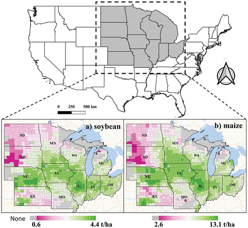
This study focuses on the Midwestern United States (Figure 1), which comprises 959 counties across 12 states. The US Midwest Region is known as the primary producer of soybeans and maize in the United States, contributing a substantial 83.5% and 85.9% of the national total soybean and maize production in 2021, respectively. This region exhibits diverse soil compositions, climatic variations (Shahhosseini et al. 2019), varying irrigation intensities, and a wide range of agricultural practices. These diverse conditions have led to considerable variation in the average soybean yields (ranging from 0.6–4.4 t/ha) and maize yields (ranging from 2.6 to 13.1 t/ha) across counties from 2004 to 2021 (Figure 1). The central part of the study area typically has higher soybean and maize yields, while the northern Great Plains have lower regional average yields. Crucially, the Midwestern United States has consistent and reliable statistical data concerning maize and soybean yields. This robust dataset serves as a cornerstone in advancing the development of predictive models for both maize and soybean yields. As a result, trials in this area can deliver compelling results.

Figure 1. Average yields of (a) soybean and (b) maize in the Midwestern United States, 2004–2021.

2.1. Data

2.1.1. Historical yield records

To ensure consistency and completeness, historical yield records of soybean and maize from 2004–2021 in the Midwestern U.S. were obtained from the Quick Stats Database of the United States Department of Agriculture (USDA), National Agricultural Statistics Service (NASS). Notably, an upward trend was observed in both crop yields from 2004–2021 (Figure 2). The significant fluctuations in crop yields across years were primarily due to varying weather conditions and other contributing factors.

Figure 2. Historical yield records of a) soybean and b) maize in the Midwestern U.S., 2004–2021.

Crop yield anomalies occurred in 2008, 2012, 2016, and 2019. Specifically, the droughts that occurred in 2008 and 2012 significantly reduced soybean yields. The impact of the 2012 drought on corn yields was more pronounced due to the relatively weaker drought tolerance of corn than that of soybeans (Rippey 2015). Conversely, the weather conditions in 2016 were favorable for soybean, resulting in a record high soybean yield. In 2019, heavy spring rains and flooding in the Midwest caused delays in the planting of soybean and maize (Shahhosseini et al. 2019), resulting in reduced yields of soybean and maize.

To establish a more comprehensive trend analysis, we extended our examination to include a wider historical yield range spanning from 1980–2021. By employing a linear model, y = α×year+β, where y represents the soybean or corn yield for a specific county in a given year, “year” denotes the harvest year, and α and β are parameters specific to the scale and crop, respectively, we assessed the overall fit quality and significance level of the model through an F test, R² and p values. Our findings indicated a notable and significant increase in both soybean and maize yields across the Midwest during this extended timeframe. The linear rate of increase was calculated to be 0.036 t/ha per year for soybean (N = 33309, R² = 0.344, p < 0.001) and 0.135 t/(ha•year) for maize (N = 36193, R² = 0.404, p < 0.001).

2.1.2. Crop layers

In this study, the cropland data layer (CDL) data from 2008 onward was used to differentiate maize (code = 1) and soybean (code = 5) pixels within each county (Boryan et al. 2011). Prior to 2008, the maize-soy data layer (CSDL) data were employed, as detailed in (S. Wang et al. 2020). The CSDL dataset was generated using machine learning techniques, leveraging training samples from the CDL to address missing maps of CDL for specific states in the Midwestern region before 2008.

2.1.3. Satellite and climate data

The satellite data used in this study include three main datasets: MOD09A1 (Vermote 2015), MOD11A2 (Wan, Hook, and Hulley 2015), and MOD16A2 (Running, Mu, and Zhao 2017). The seven surface reflectance and spectral indices provided comprehensive insights into the conditions of the soybean and maize crops. The dynamic climate data from the GRIDMET DROUGHT (Abatzoglou 2013) and NLDAS-2 (Cosgrove et al. 2003) datasets are used to measure the environmental stresses during soybean and maize growth. These datasets are extensive and openly available and have been preprocessed to extract the county-level and time-based features using the Google Earth Engine (GEE) (Gorelick et al. 2017). The specifics of the satellite and climate data are outlined in Table 1.

Table 1. Summary of bands from the satellite and climate datasets.

Data sources	Bands	Formulation/Wavelength/Description	Frequency	Resolution
MOD09A1	Red	620–670 nm	8-day	500 m
	Nir	841–876 nm
	Blue	459–479 nm
	Green	545–565 nm
	Nir_1	1230–1250 nm
	Swir1	1628–1652 nm
	Swir2	2105–2155 nm
	LSWI	Land surface water index, (Nir-Swir1)/(Nir+Swir1)
	NDVI	Normalized difference vegetation index, (Nir-Red)/(Nir + Red)
	EVI	Enhanced Vegetation Index, 2.5× (Nir-Red)/(Nir+6*Red-7.5*Blue+1)
	GCVI	Green chlorophyll vegetation index, Nir/Green − 1
	SAVI	Soil adjusted vegetation index, 1.5×(Nir-Red)/(Nir+Red+0.5)
MOD11A2	LSTDay	Day land surface temperature	8-day	1000 m
	LSTNight	Night land surface temperature
MOD16A2	ET	Evapotranspiration	8-day	500 m
GRIDMET DROUGHT	SPI	standardized precipitation index was aggregated for the last 14days	daily	4638.3 m
	EDDI	Evaporative demand drought was aggregated for the last 14 days
	SPEI	Standardized precipitation evapotranspiration index was aggregated for the last 14 days
	PDSI	Palmer Drought Severity Index
	Palmer_Z	Palmer Z Index
NLDAS-2	Precipitation	Hourly total precipitation	hourly	13915 m
	Temp	Air temperature at 2 meters above the surface
	Humidity	Specific humidity at 2 meters above the surface
	Pressure	Surface pressure
	Longwave	Surface downward longwave radiation

The preprocessing of surface reflectance and spectral indices from the remote sensing data involved several steps. These steps included quality assessment, pixel masking for non-soybean or non-maize areas, 10-day compositing, temporal reconstruction, and county aggregation. The following steps were carried out to ensure the highest quality:

1. Cloud-contaminated pixels were initially masked using the quality band. Subsequently, the pixels lacking soybean or maize coverage were masked using the CDL and CSDL datasets.

2. Band information within the datasets was composited for each pixel using a 10-day average approach.

3. Linear moving interpolation (Griffiths, Nendel, and Hostert 2019) was applied to fill missing values attributed to cloud interference for each pixel.

4. Ultimately, the data were aggregated at the county level, generating time-based features for all countries cultivating soybean or maize.

2.1.4. Phenology information

The phenology-based features were derived from the time-based features by segmenting the growth cycles of soybeans and maize into distinct phenological stages. Soybeans have six stages: planting, emerging, blooming, podding, leaf dropping, and harvesting. Maize, on the other hand, has seven phases: planting, emergence, silk production, kernel development, denting, maturity, and harvest (source: https://usda.library.cornell.edu/). Weekly phenology data were sourced from crop progress reports across various states. These reports assess the percentage of land in different phenological stages and contain contributions from approximately 3600 investigators.

To obtain more granular data, weekly phenology records were transformed into daily phenology data using cubic polynomial interpolation. The resulting data were more detailed and could provide a better understanding of crop growth patterns. This process involved resampling the originally recorded weekly crop progress. The phenological period in each state was defined as the period between 25% and 75% phenological progress. During this period, time-based features were aggregated, either by averaging or summing, to generate new phenology-based features. This approach ensured that the data cover key growth stages, thereby improving the understanding of crop development and performance.

2.1.5. Auxiliary data

The auxiliary data used in this study included irrigation percentage and geo-location information; these were assumed to be constant over time or to change infrequently. The USDA compiled data on irrigated and non-irrigated cropland for the years 2002, 2007, 2012, and 2017; these data were collected every five years as part of the census. Due to substantial missing data at the county level for non-census years, the closest five-year values of the percentage of irrigated cropland (PIC) were assigned as an explanatory variable. The PIC is defined as the ratio of irrigated cropland area to total cropland area, and the PIC serves as an indicator of a county’s irrigation level. PIC values for specific years were sourced from corresponding census years: 2003 and 2004 from the 2002 census; 2005, 2006, 2008, and 2009 from the 2007 census; 2010, 2011, 2013, and 2014 from the 2012 census; and 2015, 2016, 2018, 2019, 2020, and 2021 from the 2017 census. The spatial distribution of soybean and maize yields was analyzed using the shapefile data, which included each county’s centroid latitude and longitude along with its state, to elucidate the spatial distribution of soybean and maize yields.

To prepare the input for the model, both dynamic and static features were merged into a large matrix. In this study, a normalization technique was employed to mitigate the variations in the feature magnitudes and to optimize the model performance. Specifically, the Z score method (Jain et al. 2005) was utilized to transform numerical features into a standard normal distribution, aligning with the typical requirements of machine learning algorithms for optimal performance (Raju et al. 2020). In addition, we chose to use a string-based state feature as a predictor to reflect the differences in the agricultural technology between states and to better capture the substantial spatial variation in the maize and soybean yields. This string feature was transformed into 12 binary features through one-hot encoding. To improve the interpretability of the results, 200 influential features (excluding the trend features) were selected based on the feature importance of the XGBoost algorithm.

2.2. Methodology

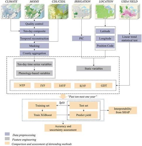
In our previous study (Li et al. 2023), we extensively compared the performance of various machine learning and deep learning models for soybean yield prediction within the U.S. Midwest region. Based on this analysis, the XGBoost algorithm was selected to construct a soybean yield prediction framework. Expanding on this framework, our current study aims to examine the impact of yield detrending on the prediction accuracy, broadening our predictive scope to encompass both soybean and maize crops. Figure 3 shows the flowchart with an overview of our methodology. Section 2.1 describes the intricate process of data preprocessing and feature engineering this process is crucial for generating the dynamic and static variables essential for the yield prediction. Additionally, different detrending methods are comprehensively compared and evaluated, with an interpretability analysis of the machine learning models using SHAP.

Figure 3. Flowchart of the soybean and maize yield prediction at the county level under the five detrending scenarios employing an XGBoost-based model.

2.2.1. Detrend processing methods

We categorized detrending methods into five groups:

(1) No trend processing (NTP): This group retains the interannual trend without removal. The mathematical representation is as follows:-

(1) ${\hat{y}}_{\mathit{i}}=\mathit{f}\left({\mathit{x}}_i\right)$(1)

where ${\mathit{x}}_i$ denotes the vector input corresponding to the $i^{\mathit{th}}$ sample. $\mathit{f}$ is defined as the function of the XGBoost algorithm. The output$\mathit{\hspace{0.17em}}{\hat{y}}_{\mathit{i}}$ symbolizes the predicted yield value for the $i^{\mathit{th}}$ sample.

(2) Input year as a feature (IYF): The mathematical representation is as follows:-

(2) ${\hat{y}}_{\mathit{i}}=\mathit{f}\left([{\mathit{x}}_i,\mathit{yea}{r}_i]\right)$(2)

where $\mathit{yea}{r}_i$ represents the harvest year of the $i^{\mathit{th}}$ sample, acting as a new dimension in the input vector ${\mathit{x}}_i$. For the whole input matrix, $\mathit{x}$ is equivalent to effectively adding a new column to represent the year.

(3) Input average yield as a feature (IAYF): The mathematical representation is as follows:-

(3) ${\hat{y}}_{\mathit{i}}=\mathit{f}\left([{\mathit{x}}_i,\mathit{av}{e}_{\mathit{i},\mathit{j}}]\right)$(3)

where $\mathit{av}{e}_{\mathit{i},\mathit{j}}$ is the average historical yield from the previous $\mathit{j}$ years before the test year of the $i^{\mathit{th}}$ sample, and $\mathit{j}=5$.

(4) Input linear yield as a feature (ILYF) (Medina, Tian, and Abebe 2021; Shahhosseini et al. 2021). The mathematical representation is as follows:-

(4) ${\hat{y}}_{\mathit{i}}=\mathit{f}\left([{\mathit{x}}_i,\mathit{ln}{r}_{\mathit{i},\mathit{j}}]\right)$(4)

where $\mathit{ln}{r}_{\mathit{i},\mathit{j}}$ represents the linear trend yield in the test year calculated for the $i^{\mathit{th}}$ sample based on the previous $\mathit{j}$ years, and $\mathit{j}=30$.

(5) Global detrending (GDT): The mathematical representation is as follows:-

(5) ${\hat{y}}_{\mathit{i}}=\mathit{f}\left({\mathit{x}}_i\right)-{\alpha }_j\mathit{year}-{\beta }_j$(5)

where ${\alpha }_j$ is the slope obtained by fitting a linear model to the historical yields for $\mathit{j}=30$ years before the test year, and ${\beta }_j$ is a constant term. ${\alpha }_j$ and ${\beta }_j$ will be slightly different for each test year.

2.2.2. Algorithm: XGBoost

XGBoost is an innovative tree-based ensemble algorithm pioneered by Chen and Guestrin (2016). XGBoost is characterized by high-speed parallel computational capabilities and a robust design that mitigates overfitting through features such as early stopping, L1 and L2 regularization terms of the loss function, and tree pruning (Chen and Guestrin 2016). It has emerged as an exceptionally effective solution for tabular data, consistently outperforming various machine learning and even cutting-edge deep learning models in recent reviews (Borisov et al. 2022; Grinsztajn, Oyallon, and Varoquaux 2022). Moreover, XGBoost is resilient to multicollinearity among highly correlated features (Chen and Guestrin 2016). Notably, XGBoost has outperformed popular algorithms such as random forest (RF), long short-term memory (LSTM), and deep neural network (DNN) algorithms in numerous yield studies (Li et al. 2023).

The model employed in this study was XGBRegressor. Certain hyperparameters were empirically set to ensure a more conservative model. These included the following: max_depth of 7, defining the maximum depth of a tree; min_child_weight of 3, used as the stopping criterion for splitting nodes; learning_rate of 0.09, employed as a shrinkage step size to prevent overfitting; n_estimators of 700, signifying the number of trees; objective = “reg:gamma,” serving as the objective function for “reg:gamma;” colsample_bytree of 0.7, determining the subsample ratio of columns when building each tree; reg_alpha of 0.1, employed as the L1 regularization term on weights; and subsample = 0.8, defining the subsample ratio of the training instances. Default values were retained for the remaining hyperparameters.

2.2.3. Performance assessment

To assess prediction uncertainty, 10 training and testing cycles were used, each with unique random seed parameters (9, 19, 29, 39, 49, 59, 69, 79, 89, and 99). Since the yield prediction accuracy and uncertainty significantly vary each year, relying on a single year’s yield as a test set can introduce bias. Hence, the training and test sets were divided based on an “N + 1” strategy and N was fixed to 10. The “N + 1” strategy is where the upcoming year’s yields and features were the test set and data from the previous ten years served for training, and this strategy was chosen to minimize bias (Paudel et al. 2021). This approach, unlike the “leave-one-year-out” strategy (Sakamoto 2020), avoided temporal irreversibility by using future data to predict past yields.

The evaluation metrics for model performance included R² and the root-mean-square error (RMSE); these metrics were calculated for the test years. R² is the percentage of variability in the statistical yields explained by the predicted yields, with a value closer to 1 indicating better performance. The RMSE reflects the average prediction error, with a smaller value indicating better performance, and is generally larger than the mean absolute error (MAE). The results are presented as the mean ± standard deviation, which reflects both the accuracy and uncertainty of the model’s predictions. Each training and test iteration was repeated ten times with different random seed parameters to ensure robustness and reliability in the evaluation process.

2.2.4. Interpretability of SHAP

SHAP (Lundberg and Lee 2017) is an approach that aims to explain the output of machine learning models by assigning each feature an importance value for a particular prediction. It is rooted in game theory and calculates the contribution of each feature to the prediction, allowing for a more granular understanding of how the individual features impact the model’s output. SHAP values provide insights into why a model makes a specific prediction, enhancing interpretability and transparency, especially in complex models such as deep learning and ensemble methods.

One innovation of SHAP is that it represents the Shapley value explanation as an additive feature attribution method similar to a linear model. It quantifies the contribution of each feature to the model’s prediction by considering all potential combinations of the feature values and weighting them accordingly, as demonstrated in Eq.(6)(6) ${\varphi }_j\left(\mathit{val}\right)=\sum _{\mathit{S}\subseteq \left\{1,\dots ,\mathit{p}\right\}\setminus \left\{j\right\}}\frac{\left|\mathit{S}\right|!\left(\mathit{p}-\left|\mathit{S}\right|-1\right)!}{\mathit{p}!}\left(\mathit{val}\left(\mathit{S}\cup \left\{\mathit{j}\right\}\right)-\mathit{val}\left(\mathit{S}\right)\right)$(6) (Štrumbelj and Kononenko 2013):-

(6) ${\varphi }_j\left(\mathit{val}\right)=\sum _{\mathit{S}\subseteq \left\{1,\dots ,\mathit{p}\right\}\setminus \left\{j\right\}}\frac{\left|\mathit{S}\right|!\left(\mathit{p}-\left|\mathit{S}\right|-1\right)!}{\mathit{p}!}\left(\mathit{val}\left(\mathit{S}\cup \left\{\mathit{j}\right\}\right)-\mathit{val}\left(\mathit{S}\right)\right)$(6)

where ${\varphi }_j\left(\mathit{val}\right)$ is the contribution of feature $\mathit{j}$ via a value function $\mathit{val}$, $\mathit{S}$ is the subset of the features incorporated into the model, and $\mathit{x}$ represents the feature vector of the instance being explained. Additionally, $\mathit{p}$ represents the total number of features. $\mathit{va}{l}_x\left(\mathit{S}\right)$ represents the prediction for the feature values within set $\mathit{S}$, factoring in the marginalization over features not encompassed in set $\mathit{S}$:-

(7) $\mathit{va}{l}_x\left(\mathit{S}\right)=\int \hat{f}\left(x_1,\dots ,x_p\right)\mathit{d}{P}_{\mathit{x}\notin \mathit{S}}-E_X\left(\hat{f}\left(\mathit{X}\right)\right)$(7)

where $\hat{f}\left(\mathit{x}\right)$ represents the prediction for feature vector $\mathit{x}$, and $E_X\left(\hat{f}\left(\mathit{X}\right)\right)$represents the mean prediction.

The Shapley value for a specific feature quantifies the average change in predictions made by existing features in the room when that feature is included. Specifically, when the $\mathit{j}$-th feature enters the room, the features already in the room have $\left|\mathit{S}\right|!$ possible orders, while the features that are not yet in the room have $\left(\mathit{p}-\left|\mathit{S}\right|-1\right)!$ possible orders. The weight of the $\mathit{j}$-th feature when it enters the room is given by $\frac{\left|\mathit{S}\right|!\left(\mathit{p}-\left|\mathit{S}\right|-1\right)!}{\mathit{p}!}$.

3. Results

3.1. Performance of the yield prediction with different detrend processing methods

A comparison of the performances of the five detrending methods is provided in Table 2. The application of detrending to historical yield records significantly improved the accuracy and reduced the uncertainty in predicting soybean and maize yields; this is indicated by both the RMSE and R² values. Table 2 shows that the NTP method resulted in the poorest yield prediction, with an average prediction error of 0.396 t/ha for soybean and 1.175 t/ha for maize, explaining only 53.4% and 53.5% of the statistical yield variability, respectively. On the other hand, the prediction accuracy for the other four detrending groups (IYF, IAYF, ILYF, and GDT) notably improved in comparison to that of the NTP group. The ranking order of the four detrending groups by performance was as follows: GDT > ILYF > IAYF > IYF. The IYF method showed the poorest performance among the four detrending groups. However, compared with the NTP method, this method improved the R² by 0.079 for soybean and 0.069 for maize and reduced the average RMSE by 0.035 t/ha for soybean and 0.08 t/ha for maize. The GDT group exhibited the best performance, with the predicted result closer to the statistical yield for soybean (3.378 t/ha vs. 3.441 t/ha) and maize (10.869 t/ha vs. 10.834 t/ha). In terms of R² and RMSE, GDT improved the R² by 0.206 and 0.196 for soybean and maize, respectively, and reduced the average yield prediction error by 0.091 t/ha and 0.158 t/ha for soybean and maize, respectively.

Table 2. Average prediction accuracy for the soybean and maize yield of five groups from 2014 to 2021.

Detrending	Soybean			Maize
	Prediction(t/ha)	RMSE(t/ha)	R^2	Prediction(t/ha)	RMSE(t/ha)	R^2
NTP	3.180	0.396±0.055	0.534±0.229	10.103	1.175±0.125	0.535±0.172
IYF	3.238	0.361±0.051	0.613±0.199	10.225	1.095±0.080	0.604±0.121
IAYF	3.289	0.319±0.052	0.690±0.188	10.378	1.015±0.075	0.661±0.090
ILYF	3.290	0.314±0.047	0.702±0.163	10.441	0.964±0.053	0.695±0.077
GDT	3.378	0.305±0.035	0.740±0.080	10.869	0.917±0.070	0.731±0.045
Statistical	3.441	–	–	10.834	–	–

The ranking of the standard deviation of the RMSE concerning uncertainty followed the sequence NTP > IYF > IAYF > ILYF > GDT. Despite the slight discrepancy between the RMSE and R² accuracy rankings, this sequence remained consistent. The NTP method exhibited the greatest deviation in yield prediction, with standard deviations in RMSEs of 0.055 t/ha and 0.125 t/ha for soybean and maize, respectively. The R² values for the soybean and maize yield predictions also fluctuated, with standard deviations of 0.229 and 0.172, respectively, indicating a high level of uncertainty. In contrast, the GDT method was found to be the most stable method, significantly reducing the standard deviation of the RMSE to 0.035 t/ha for soybean and 0.070 t/ha for maize. Furthermore, compared to NTP, GDT minimized the standard deviation of R² to 0.08 for soybean and 0.045 for maize These results indicated that the GDT method was better suited for yield prediction, as it produced more accurate and stable results than the other methods.

3.2. Yield prediction accuracy across years

3.2.1. Interannual variation in prediction accuracy

Figure 4 illustrates the performance of the five groups from 2014 to 2021 in predicting soybean and maize yields (Figure 4a–d). The results indicate substantial variations across different years. In 2016, all five groups displayed relatively poor performance in predicting soybean yield, achieving an average R2 of only 0.243. Similarly, the year 2019 had the lowest predictive accuracy for maize yield among the five groups, and the groups achieved an average R2 of 0.50. Conversely, the model exhibited remarkable accuracy and consistency in predicting both soybean and maize yields in 2021, with all five groups yielding average R2 values of 0.850 for soybean and 0.825 for maize. A method capable of capturing the variability in interannual yield predictions is highly important to ensure accurate and reliable predictions.

Figure 4. Performance comparison of the yield prediction by the 5 detrending methods (NTP, IYF, IAYF, ILYF, and GDT) from 2014–2021. A) R² of the soybean yield predictions, b) RMSE of the soybean yield predictions, c) R² of the maize yield predictions, and d) RMSE of the maize yield predictions.

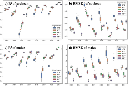
Despite considerable interannual variation, the prediction accuracy generally followed a consistent ranking across most years: NTP <IYF<IAYF<ILYF<GDT. During the periods of soybean yield prediction from 2014 to 2016 and maize yield prediction from 2016 to 2020, GDT notably outperformed the other groups, yielding acceptable predictions based on the RMSE and R² results (Figure 4). However, the differences among IAYF, ILYF and GDT were marginal from 2017 to 2020 for soybean yield prediction but notably surpassed that of IYF and subsequently outperformed NTP. In 2021, all groups performed well, with no distinct differences observed among the five detrended groups.

The consistency in the maize yield prediction accuracy typically followed this trend across most years: NTP < IYF < IAYF < ILYF < GDT. This pattern was notably apparent from 2016 to 2020, when the low R² value of the NTP showed a substantial influence to the interannual yield trends on the predictions during these periods. In 2015, IAYF, ILYF, and GDT outperformed NTP and IYF, but no significant difference was found between NTP and IYF. However, similar to soybean yield predictions, there was no evident superiority among the five groups in 2021.

A clear trend emerged when comparing the annual average county-level yield forecasts of the five groups with the NASS statistical results. Over the years from 2014–2021 (Table 3), GDT consistently showed superior performance in soybean yield prediction compared to the other four groups. Conversely, NTP consistently ranked as the weakest performer for soybean yield prediction in most years.

Table 3. Annual average predictions and statistical values for soybean yield.

Year	Statistics(t/ha)	Prediction(t/ha)
		NTP	IYF	IAYF	ILYF	GDT
2014	3.271	3.103	3.102	3.123	3.122	3.231
2015	3.392	3.104	3.125	3.143	3.170	3.329
2016	3.672	3.238	3.279	3.295	3.324	3.435
2017	3.397	3.115	3.259	3.229	3.262	3.330
2018	3.530	3.232	3.324	3.359	3.363	3.434
2019	3.257	3.033	3.104	3.256	3.240	3.218
2020	3.485	3.213	3.282	3.365	3.324	3.444
2021	3.524	3.407	3.433	3.545	3.518	3.602

Note: light green indicates the best predicted result, and yellow indicates the poorest predicted result.

Similar discernible trends emerged in the maize yield predictions(Table 4), where GDT outperformed the other groups in almost all years, while NTP consistently ranked as the weakest performer for most years from 2014 to 2021. These comparisons highlighted the importance of yield detrending in machine learning for crop yield prediction and showed the superior performance of GDT over the other four methods.

Table 4. Annual average predictions and statistical values for maize yield.

Year	Statistics(t/ha)	Prediction(t/ha)
		NTP	IYF	IAYF	ILYF	GDT
2014	10.644	10.144	10.170	10.093	10.174	10.737
2015	10.373	9.921	9.937	10.042	10.171	10.584
2016	10.941	10.051	10.186	10.181	10.346	10.952
2017	11.079	10.135	10.329	10.350	10.521	10.879
2018	11.276	10.503	10.596	10.905	10.893	11.129
2019	10.685	9.674	9.844	10.231	10.237	10.451
2020	10.761	9.898	10.252	10.369	10.385	10.987
2021	10.914	10.500	10.484	10.851	10.798	11.232

Note: light green indicates the best predicted result, and yellow indicates the poorest predicted result.

3.2.2. Differences in the predictions from the five detrending methods for unusually low yields in 2016 and 2019

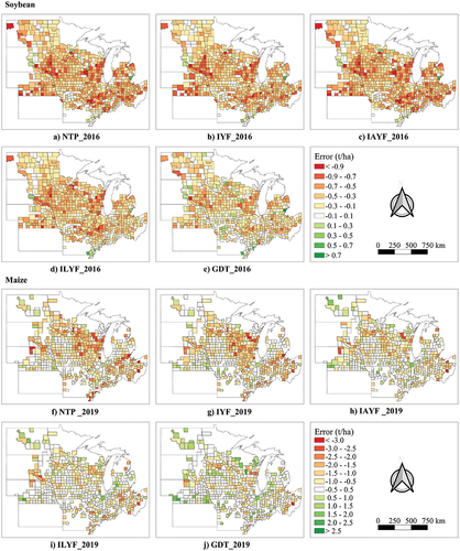
In 2016, the model encountered challenges in accurately predicting soybean yield due to the exceptionally high yield of soybean in this year. Similarly, the precision of the model was impacted in 2019 due to unusually low yields of maize. The error plots for the 2016 soybean yield prediction and the 2019 maize yield prediction (seed = 99) for the five groups are presented in Figure 5. The red on the plot indicates that all five groups underestimated the soybean yield for most counties in 2016. Conversely, the predicted maize yields in 2019 were lower than the statistical yields in the central and eastern regions and slightly greater than those in North Dakota and southern Nebraska. Notably, ILYF and GDT substantially diminished the magnitude of the error, as indicated by the lighter colors on the graph. In particular, GDT notably minimized the magnitude of errors, especially in counties across southern Wisconsin, southeastern South Dakota, and central Illinois. This pattern highlights the importance of continuous improvement in detrending methodologies to minimize error and improve accuracy in yield predictions.

Figure 5. Spatial distribution of the yield prediction errors (predicted value – statistical value) for soybean (2016) and maize (2019) using the 5 detrending methods (NTP, IYF, IAYF, ILYF, and GDT).

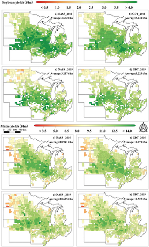
The predicted yields for soybean and maize in 2016 and 2019 using GDT are illustrated in Figure 6. In general, the soybean and maize yield predictions derived from GDT closely aligned with the spatial distribution of yields reported by NASS statistics. The central regions of the Great Plains consisting of NE, IL, IA, and IN emerged as high-yielding areas for soybean and maize, while the peripheral areas, notably the ND and SD, exhibited lower yields. A comparison of the predicted yields derived from GDT to the statistical yields obtained from NASS showed notably high R² values. In 2016, the R² values were 0.77 for soybeans and 0.73 for maize. Similarly, in 2019, the R² values were 0.76 for soybeans and 0.69 for maize.

Figure 6. Spatial contrast of the predicted yields utilizing GDT against NASS statistical yields for soybean and maize in 2016 and 2019.

In summary, the detrending treatments demonstrated a notable improvement in prediction accuracy and a reduction in uncertainty during the unusual yield years 2016 and 2019. Specifically, the GDT method exhibited effectiveness in enhancing the accuracy and minimizing uncertainty during anomalous yield periods. Based on these findings, we recommend the adoption of the GDT method to predict crop yield, especially in abnormal yield years.

3.3. Interpretability of the yield prediction model

The SHAP analysis results for soybean and maize yield predictions for 2016, 2019, and 2021 are shown in Figures 7 and 8, respectively. The feature analysis of IYF, IAYF and ILYF, as opposed to NTP, showed the critical importance of the yield trends for XGBoost. In the figures, the top ten features are ranked from highest to lowest impact on the predictions.

Figure 7. SHAP values of the soybean yield predictions for 2016, 2019, and 2021; the horizontal axis represents the SHAP values affecting the model output.

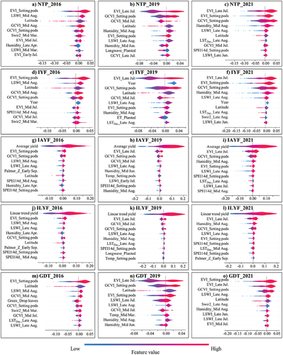
Figure 8. SHAP values of the maize yield predictions for 2016, 2019, and 2021; the horizontal axis represents the SHAP values affecting the model output.

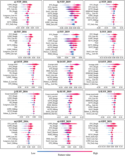
As shown in Figures 7g–i and 8g–i, the features representing the average yield of the last five years had the highest average absolute SHAP values, indicating their significant influence. Similarly, ILYF in Figures 7j–l and 8j–l revealed the significant impact of the linear trend yield feature derived from the past 30 years on the yield prediction. These findings were consistent with the results from Shahhosseini et al. (2020); they identified the “yield_trend” and “yield_avg” as the top 2 features for the maize yield prediction in the corn belt using an optimized weighted ensemble. While the year feature ranked among the top 10 predictors for the soybean and maize predictions in 2016, 2019, and 2021 in IYF (Figures 7d–f and 8d–f), its significance was notably surpassed by the average yield in IAYF and the linear trend yield in ILYF. These findings showed the pivotal role of the average yield and linear trends in achieving precise yield predictions. However, using only the year to represent a trend is not as powerful as incorporating the average yield and linear trend yield; this accentuates the model’s limited capacity to independently learn yield trends through the year feature alone.

The second key finding of the feature analysis highlighted the significance of the EVI in predicting the soybean and maize yields. The satellite spectral indices and meteorological indicators contributed to the yield variability. Among these, the EVI emerged as a vital feature following the trend feature, with higher EVI values correlating to increased yields. Notably, the EVI during the podding stage of soybean and the dough stage of maize was of utmost importance. Soybean podding typically occurred between July 20 and August 10, and the maize dough stage occurred between July 30 and August 20 in each state. This observation was consistent with the timing of flowering in soybean and maize. Nevertheless, while the EVI was significant, it was not dominant as the trend feature was. Other vegetation indices (e.g. GCVI and LSWI), meteorological indices (e.g. humidity, LST, and PDSI), and geolocation features (e.g. latitude) also contributed substantially to the yield prediction.

Third, the most important phenological period influencing yield prediction was identified as the podding stage for soybean and the dough stage for maize. The SHAP plots highlighted the top 10 influential features centered on soybean podding and maize dough, particularly in mid-July, late July, early August, mid-August, and late August. This finding provides valuable information for future feature selection for the yield prediction.

Furthermore, the impact of spectral indices on yield prediction was more significant than that of meteorological indices.

Most spectral indices exhibited a positive correlation with the yield prediction. For example, a higher EVI during the podding stage corresponded to higher predicted yields from the model. However, latitude, the daytime land surface temperature in late August (LST_Day_late Aug.) and the longwave radiation were negatively correlated with the predicted soybean yield. During the maize silking period in 2019, the PDSI significantly varied from 2016–2021, ranking among the top 10 features and showing a negative correlation with yield. The model predicted reduced maize yield with higher PDSI values.

4. Discussion

Our findings showed the substantial improvement in accuracy and reduction in uncertainty when integrating the yield trends as a feature compared to models employing the NTP method. Machine learning models are inherently probabilistic due to various factors, such as weight initialization, objective function optimization, and hyperparameter tuning (Bouthillier et al. 2021). Additionally, uncertainties in yield prediction result from the observational noise and are influenced by interannual and seasonal variabilities in environmental stressors, such as heat and water stress. Models lacking detrending tend to exhibit wider confidence intervals, which can lead to diminished generalization performance when predicting future crop yields. To improve the prediction accuracy, yield trends need to be incorporated into models. Previous studies have consistently emphasized the importance of incorporating yield trends to improve prediction accuracy. For instance, Shahhosseini et al. (2019) demonstrated a 4% improvement in R² by incorporating the previous five-year average yield as a feature (IAYF). Similarly, Shahhosseini et al. (2021) identified the substantial impact of the linear trend yield features on the yield prediction using machine learning models. Wang et al. (2020b) utilized GDT and observed a remarkable increase in the prediction R², which increased from 0.23–0.77 after detrending.

4.1. The performance comparison between XGBoost and other five algorithms

In this study, we selected the XGBoost algorithm to compare the yield prediction performance of five detrending algorithms. We further compared the soybean and maize yield prediction performance from 2014–2021 by RF, artificial neural network (ANN) with three layers, support vector regression (SVR) (Noble 2006), LSTM, DNN and XGBoost. The value of R² and RMSE indicated that XGBoost outperformed the other five algorithms in almost all years (Tables A1–A4), which supported the rationality of choosing XGBoost as the benchmark algorithm to evaluate the performance difference among the five detrending process methods. It is worth noting that machine learning algorithms have evolved rapidly in recent years and new algorithms are emerging. This suggests that XGBoost may not remain the best algorithm for crop yield prediction. Consequently, when attempting to predict crop yields, Hence, it is essential to compare the performance of various algorithms for better crop yield prediction.

4.2. Outstanding performance using GDT for the abnormal yield years

In our analysis, IAYF and ILYF performed well and provided easily interpretable results. However, GDT achieved the most substantial improvement in both accuracy and uncertainty, particularly in years with unusual crop yields. To further assess the effectiveness of GDT in crop yield prediction in abnormal scenarios, we examined the relationship between the absolute error and deviation trend yield between NTP and ILYF and between NTP and GDT in all years spanning from 2014–2021 (refer to Figure 9). The deviation from the expected trend yield indicates the absolute difference between the predicted trend yield and the actual statistical yield for each predicted year. For instance, the trend yield for 2022 was determined by the formula α_j *2022+β_j, where α_j and β_j denote fitted values from equation (5)(5) ${\hat{y}}_{\mathit{i}}=\mathit{f}\left({\mathit{x}}_i\right)-{\alpha }_j\mathit{year}-{\beta }_j$(5) . By using this approach, the limitations of specific years were able to be overcome, and a more focused and comprehensive comparison among NTP, ILYF, and GDT was provided.

Figure 9. Relationship between the absolute error of soybean and maize after detrending with ILYF and GDT and the deviation from the trend yield.

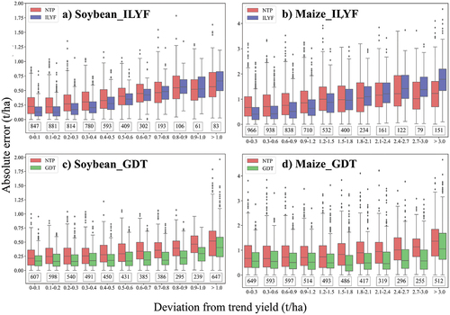
Our findings can be summarized as follows:

• Both GDT and ILYF demonstrated effectiveness in reducing the absolute error across the various deviation levels. These results highlighted the significance of incorporating detrending techniques to improve the accuracy of yield predictions.

• When the deviation was less than 0.4 t/ha for soybeans and 1.2 t/ha for maize, the absolute error reduction of ILYF with respect to NTP remained stable. However, when deviations exceeded this threshold, the reduction in absolute error for ILYF became significantly lower or even surpassed that of NTP. These results indicated that ILYF might not perform as well in highly abnormal years.

• Conversely, GDT consistently outperformed NTP in terms of the average absolute error across all deviation levels, regardless of whether it was for soybeans or maize. Specifically, when using GDT to predict the soybean yield with a deviation of less than 1.0 t/ha or maize yield with a deviation of less than 3.0 t/ha, the absolute error decreased as the deviation increased. Essentially, GDT effectively minimized errors in the abnormal yield samples.

The mechanism of yield formation is complex and influenced by many factors. Advancements in agricultural technology could lead to significant yield increases over the years. However, climate variation and natural disasters within a year could cause significant yield fluctuations in a particular year. Therefore, an accurate yield forecasting method should be able to simultaneously predict these two characteristics. Compared to other detrending methods, GDT could significantly reduce the impact of agricultural technology on the crop yield and enable the machine learning algorithms to better capture the yield variation caused by meteorological factors, stress, and vegetation conditions. Based on this analysis, GDT was most effective in the abnormal years, such as 2016 and 2019, as the coupling of trends and fluctuations was most pronounced in these years.

4.3. Model interpretation for understanding the yield predictors

Notably, while SHAP values provide insights into how the model makes decisions, they also show the correlations between the features and predicted yields. The SHAP framework highlighted the EVI as the most influential predictor of year-to-year fluctuations, which could be attributed to its ability to reflect the vegetation stress of soybean and maize by mitigating the soil background and atmospheric effects through the incorporation of blue bands (Huete, Justice, and Liu 1994; Jiang et al. 2008; Rocha and Shaver 2009). Numerous studies have acknowledged the significance of the EVI in yield prediction (Han et al. 2020; Kim et al. 2019; Kouadio et al. 2014; Medina, Tian, and Abebe 2021). Bolton and Friedl (2013) and Peng et al. (2018) demonstrated that the EVI outperformed the NDVI, LAI, and FPAR in predicting maize yield across the Corn Belt region. Notably, not all EVIs at different phenological stages are equally important in predicting yield, with the EVIs at the soybean podding and maize dough stages being the most critical periods for accurate yield predictions of both.

Moreover, we identified latitude as a reliable predictor of the spatial variability in yield. Compared with those located farther north, counties situated at lower latitudes generally displayed higher predicted crop yields. These findings aligned with the spatial distribution of average yield in Figure 1, showing that states at lower latitudes had notably higher average yields than those at higher latitudes. For example, from 2014–2021, North Dakota reported average yields of 2.033 t/ha for soybean and 6.536 t/ha for maize; these yields were significantly lower than the average yields observed in Illinois, which is a state located at lower latitudes, and its average yields were 3.423 t/ha for soybean and 10.558 t/ha for maize.

4.4. Explanation of the GDT-predicted yields in the abnormal yield years

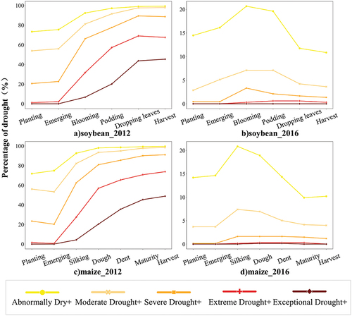
In 2012, there was a significant agricultural disaster; this disaster was the worst since 1988 and was caused by the high temperatures in late June and subsequent months of July and August. This disaster led to a loss of more than a quarter of the maize yield and production potential (Rippey 2015). During the soybean podding stage, 92% of the counties experienced drought conditions, ranging from moderate to exceptional drought. Similarly, during the maize dough stage, 93% of the counties experienced drought conditions. In contrast, 2016 was characterized by favorable weather conditions, with only 7% of counties experiencing drought conditions during both the soybean podding and maize dough stages (see Figure 10).

Figure 10. Percentage of drought with different magnitudes in the various phenological stages of soybean and maize in 2012 and 2016.

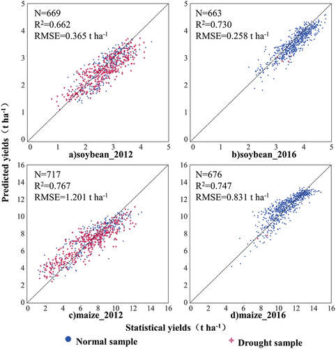
We adopted the “N + 1” strategy to assess and explore the predictive abilities of the models for these two disparate years. Scatter plots of soybean and maize yield predictions in 2012 and 2016 are presented in Figure 11, with predicted R² values of 0.662 and 0.767, respectively. Despite numerous counties experiencing extreme or very dry conditions during soybean podding or maize lactation in 2012 (the drought sample in Figure 11), the model still achieved good prediction accuracy under the “N + 1” strategy.

Figure 11. Scatterplot of the soybean and maize yield predictions in 2012 and 2016.

Figure 12 displays the top 10 features contributing to the soybean and maize yield prediction in 2012 and 2016, and the EVI during the podding stage for soybean and the EVI during the dough stage for maize were identified as the most critical features. Notably, these pivotal predictors remained consistent, indicating that the EVI was consistently the best predictor for the model’s yield prediction, regardless of whether the model experienced drought. This finding highlights the robustness and importance of the EVI as a primary indicator in both normal weather and drought years. The most notable difference between the top 10 features in 2012 and 2016 was the presence of LST_Day. In the drought year of 2012, the model relied mainly on the EVI for yield prediction but also considered additional insights from LST_Day.

Figure 12. SHAP values for the soybean and maize yield predictions for 2012 and 2016.

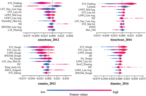
Figure 13 provides the data regarding the impact of the most influential feature, the EVI, on the yield prediction for soybean and maize. Specifically, the relationship between the EVI and its influence on yield prediction (represented by SHAP values) is shown for the years 2012 and 2016. Overall, the SHAP values demonstrate a significant and positive correlation between the yield prediction and the EVI. Notably, positive EVI values led to an increase in the predicted yield, while negative EVI values resulted in a decrease in the predicted yield. Larger EVI values resulted in a more substantial increase in output, whereas smaller EVI values led to a decrease in output. The impact of the EVI on the yield predictions was consistent across both soybean and maize. The soybean yield forecasts more closely followed this pattern, as evidenced by the absence of samples in the second and fourth quadrants of the scatter plot.

Figure 13. Interaction plot of the best features of the soybean and maize yield prediction for 2012 and 2016.

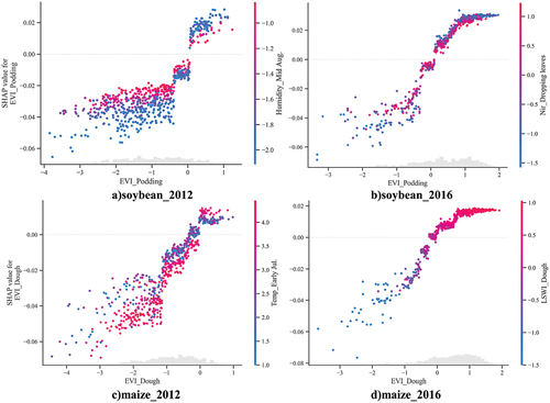
In 2012 and 2016, EVI_Podding and EVI_Dough exhibited significant differences in their most interactive features (Figure 13). In the drought year of 2012, the EVI_Podding exhibited the strongest correlation with Humidity_Late Aug., while the EVI_Dough was significantly correlated with Temp_Early Jul. These specific features of Humidity_Late Aug. and Temp_Early Jul. were directly associated with drought conditions. In 2016, a non-drought year, significant feature interactions were observed between EVI_Podding and Nir_Dropping leaves for soybean and between EVI_Dough and LSWI_Dough for maize. These results indicated two key implications: first, the EVI served as a critical indicator of vegetation impacted by drought in drought years, and second, drought-related features indirectly influenced the yield predictions by affecting the EVI.

Additionally, in the drought year (2012), the effect of the SHAP of the EVI on yield prediction also differed depending on the drought-related characteristics (Figure 13(a,c)). A negative EVI indicated drier atmospheric conditions (lower Humidity_Late Aug. and higher Temp_Early Jul.) and the model further decreased its yield prediction. These results indicated that drought primarily affected the yield prediction indirectly by affecting the EVI. On the other hand, a positive EVI occurred when the crop was growing well during the critical phenological period, and a drier atmosphere further improved the model’s yield prediction. This phenomenon potentially occurred because the crop itself was not under water stress from the natural drought due to anthropogenic interference such as irrigation; rather, the drought was accompanied by more light and could further promote photosynthesis and increase yields (Andersen, Heidmann, and Plauborg 1996).

There was a negative correlation between land surface temperature (LST) and crop yield, indicating the adverse impact of environmental heat stress on crop growth. This finding aligns with prior research demonstrating a significant decrease in crop yields under high temperatures (Hawkins et al. 2013).

4.5. Limitations

Yield trends in the United States are notably affected by advances in agricultural technology, fertilizer application, irrigation, genotype, and management (Fuglie 2007; Shahhosseini, Hu, and Archontoulis 2020). Here, we used detrending to minimize the impact of these factors on crop yield prediction. Compared to NTP, GDT significantly improved the accuracy of crop yield prediction. However, the predicted performance still needs to more improvement in the normal yield years. This highlights the importance of collecting these influencing factors from publicly available sources, considering that monitoring genetic improvements in crop seeds to increase resilience and productivity is hampered by limitations in satellite observations or ground data collection (Hussain and Thapa 2012; Shahhosseini, Hu, and Archontoulis 2020). The complexity of the coupling yield trends with climatic factors in each year causes difficult for the prediction particularly for the abnormal years with high or low yields. In this study, the training data only covered the decade prior to the prediction year, which may be insufficient for capturing extreme weather events. This mismatch between the training and prediction data could affect the generalizability of the model. This extension in historical data could strengthen the ability of models to account for extreme weather events and capture long-term trends, thereby improving prediction accuracy. In addition, the method proposed in our study is further limited by the unavailability of key input data; therefore, it cannot be used to predict future crop yields. In addition, we ignored the difference in yield trends in different sub-regions, which may be another reason why the GDT method is not good at predicting soybean yield in 2014.

5. Conclusion

In this study, we conducted a comparative analysis of five detrending methods for predicting soybean and maize yields in the Midwest United States. In our study, the importance and necessity of yield detrending in predicting crop yield using machine learning algorithms was emphasized. Yield detrending could significantly reduce the uncertainty and improve the accuracy of yield prediction for maize and soybean. GDT outperformed the other 4 detrending methods in the yield prediction of maize and soybean in the Midwestern United States, and this improvement was particularly evident during abnormal yield years. GDT notably reduced the average yield prediction error by 0.091 t/ha for soybean and 0.158 t/ha for maize with respect to NTP and concurrently improved the R² by 0.206 and 0.196 for soybean and maize, respectively. Our method could accurately predict the soybean yield from the setting pond stage and the maize yield from the dough stage in the cropping season; this was the maximum predictive ability of our method. Our results also highlighted the pivotal role of the vegetation indices, particularly the EVI during soybean podding and maize dough phenology, in predicting the crop yield fluctuations. These findings can benefit the development of machine learning models for yield prediction. In the future, we plan to enhance the global detrending method by partitioning the US Midwest into distinct agro-ecosystem zones for a more detailed analysis of the robustness. In addition, we will further conduct a comprehensive and in-depth study on the annual variability in yields to enable precise yield predictions, particularly during abnormal years.

Author contributions

Y.L. contributed to the software, analysis, and writing of the original draft of the manuscript; H.Z. conceived of the experiments and contributed to manuscript writing and the final manuscript revision; M.Z.contributed to the analysis and manuscript writing; B.W. contributed to review & editing, resources; and Q.X., contributed to the manuscript editing.

Acknowledgments

This research was supported by the National Key Research and Development Project of China (No. 2019YFE0126900), the Natural Science Foundation of China (No. 41861144019), and the Agricultural Remote Sensing Innovation Team Project of AIRCAS (No. E33D0201-6). We are very grateful for the data provided by the Quick Stats Database of the United States Department of Agriculture, National Agricultural Statistics Service; the SSURGO database of the Natural Resources Conservation Service Soils, United States Department of Agriculture; and the MODIS data from NASA. We are grateful to the editors and anonymous reviewers for their valuable comments and suggestions.

Disclosure statement

No potential conflict of interest was reported by the authors.

Data availability statement

The data that support the findings of this study are available from the corresponding author, Hongwei Zeng, upon reasonable request.

Additional information

Funding

The work was supported by the National Key Research and Development Project of China (No. 2019YFE0126900), the Natural Science Foundation of China (No. 41861144019), and the Agricultural Remote Sensing Innovation Team Project of AIRCAS (No. E33D0201-6).

Appendix

Table A1. Comparison of R² of soybean yield prediction between XGBoost and other models.

Year	RF	ANN	SVR	LSTM	DNN	XGBoost
2014	0.744	0.664	0.569	0.575	0.702	0.760
2015	0.764	0.507	0.536	0.501	0.412	0.812
2016	0.572	0.589	0.124	0.386	0.563	0.552
2017	0.781	0.697	0.607	0.628	0.774	0.807
2018	0.758	0.722	0.516	0.681	0.683	0.773
2019	0.702	0.753	0.544	0.477	0.590	0.774
2020	0.704	0.771	0.536	0.755	0.636	0.782
2021	0.795	0.828	0.660	0.793	0.795	0.850

Table A2. Comparison of RMSE (t ha⁻¹) of soybean yield prediction between XGBoost and other models.

Year	RF	ANN	SVR	LSTM	DNN	XGBoost
2014	0.277	0.317	0.360	0.357	0.299	0.268
2015	0.275	0.397	0.385	0.399	0.433	0.245
2016	0.325	0.319	0.465	0.389	0.329	0.333
2017	0.271	0.319	0.364	0.354	0.276	0.255
2018	0.326	0.350	0.462	0.375	0.373	0.316
2019	0.308	0.280	0.381	0.408	0.361	0.268
2020	0.338	0.298	0.424	0.308	0.376	0.290
2021	0.395	0.362	0.509	0.397	0.395	0.338

Table A3. Comparison of R² of maize yield prediction between XGBoost and other models.

Year	RF	ANN	SVR	LSTM	DNN	XGBoost
2014	0.760	0.702	0.780	0.701	0.598	0.776
2015	0.723	0.658	0.754	0.441	0.740	0.770
2016	0.728	0.705	0.734	0.691	0.663	0.764
2017	0.738	0.639	0.739	0.711	0.719	0.753
2018	0.727	0.650	0.678	0.717	0.643	0.758
2019	0.667	0.568	0.660	0.612	0.546	0.705
2020	0.588	0.430	0.618	0.557	0.487	0.677
2021	0.802	0.813	0.748	0.729	0.822	0.843

Table A4. Comparison of RMSE (t ha⁻¹) of maize yield prediction between XGBoost and other models.

Year	RF	ANN	SVR	LSTM	DNN	XGBoost
2014	0.839	0.937	0.805	0.907	1.088	0.812
2015	0.897	0.997	0.846	1.274	0.868	0.817
2016	0.861	0.896	0.851	0.917	0.957	0.801
2017	0.928	1.089	0.926	0.975	0.961	0.901
2018	0.963	1.090	1.047	0.980	1.101	0.906
2019	0.873	0.994	0.881	0.942	1.019	0.821
2020	1.069	1.258	1.029	1.108	1.194	0.946
2021	1.096	1.064	1.235	1.281	1.039	0.974

References

- Abatzoglou, J. T. 2013. “Development of Gridded Surface Meteorological Data for Ecological Applications and Modelling.” International Journal of Climatology 33 (1): 121–26. https://doi.org/10.1002/joc.3413.
- Andersen, M., T. Heidmann, and F. Plauborg. 1996. “The Effects of Drought and Nitrogen on Light Interception, Growth and Yield of Winter Oilseed Rape.” Acta Agriculturae Scandinavica B-Plant Soil Sciences 46 (1): 55–67. https://doi.org/10.1080/09064719609410947.
- Arata, L., E. Fabrizi, and P. Sckokai. 2020. “A Worldwide Analysis of Trend in Crop Yields and Yield Variability: Evidence from FAO Data.” Economic Modelling 90: 190–208. https://doi.org/10.1016/j.econmod.2020.05.006.
- Bailey-Serres, J., J. E. Parker, E. A. Ainsworth, G. E. D. Oldroyd, and J. I. Schroeder. 2019. “Genetic Strategies for Improving Crop Yields.” Nature 575 (7781): 109–118. https://doi.org/10.1038/s41586-019-1679-0.
- Bolton, D. K., and M. A. Friedl. 2013. “Forecasting Crop Yield Using Remotely Sensed Vegetation Indices and Crop Phenology Metrics.” Agricultural and Forest Meteorology 173: 74–84. https://doi.org/10.1016/j.agrformet.2013.01.007.
- Borisov, V., T. Leemann, K. Seßler, J. Haug, M. Pawelczyk, and G. Kasneci. 2022. “Deep Neural Networks and Tabular Data: A Survey.” Review of IEEE Transactions on Neural Networks and Learning Systems 1–21. https://doi.org/10.1109/TNNLS.2022.3229161.
- Boryan, C., Z. W. Yang, R. Mueller, and M. Craig. 2011. “Monitoring US Agriculture: The US Department of Agriculture, National Agricultural Statistics Service.” Cropland Data Layer Program Geocarto International 26 (5): 341–358. https://doi.org/10.1080/10106049.2011.562309.
- Bouthillier, X., P. Delaunay, M. Bronzi, A. Trofimov, B. Nichyporuk, J. Szeto, N. Mohammadi Sepahvand, E. Raff, K. Madan, and V. Voleti. 2021. “Accounting for Variance in Machine Learning Benchmarks.” Proceedings of Machine Learning Systems, San Jose, CA, USA, 747–769.
- Chen, T., and C. Guestrin. 2016. “XGBoost: A Scalable Tree Boosting System.” In Proceedings of the 22nd ACM SIGKDD International Conference on Knowledge Discovery and Data Mining, 785–794. Association for Computing Machinery: San Francisco, California, USA.
- Chipanshi, A., Y. Zhang, L. Kouadio, N. Newlands, A. Davidson, H. Hill, R. Warren, et al. 2015. “Evaluation of the Integrated Canadian Crop Yield Forecaster (ICCYF) Model for In-Season Prediction of Crop Yield Across the Canadian Agricultural Landscape.” Agricultural and Forest Meteorology 206: 137–150. https://doi.org/10.1016/j.agrformet.2015.03.007.
- Chlingaryan, A., S. Sukkarieh, and B. Whelan. 2018. “Machine Learning Approaches for Crop Yield Prediction and Nitrogen Status Estimation in Precision Agriculture: A Review.” Computers and Electronics in Agriculture 151: 61–69. https://doi.org/10.1016/j.compag.2018.05.012.
- Cosgrove, B. A., D. Lohmann, K. E. Mitchell, P. R. Houser, E. F. Wood, J. C. Schaake, A. Robock, et al. 2003. “Real-Time and Retrospective Forcing in the North American Land Data Assimilation System (NLDAS) Project.” Journal of Geophysical Research-Atmospheres 108 (D22). https://doi.org/10.1029/2002JD003118.
- Erenstein, O., M. Jaleta, K. Sonder, K. Mottaleb, and B. M. Prasanna. 2022. “Global Maize Production, Consumption and Trade: Trends and R&D Implications.” Food Security 14 (5): 1295–1319. https://doi.org/10.1007/s12571-022-01288-7.
- Fuglie, K. O., J. M. McDonald, V. E. Ball. 2007. Productivity Growth in US Agriculture. Washington, DC: Economic Brief Number 9, Economic Research Service.
- Gavahi, K., P. Abbaszadeh, and H. Moradkhani. 2021. “DeepYield: A Combined Convolutional Neural Network with Long Short-Term Memory for Crop Yield Forecasting.” Expert Systems with Applications 184: 115511. https://doi.org/10.1016/j.eswa.2021.115511.
- Gorelick, N., M. Hancher, M. Dixon, S. Ilyushchenko, D. Thau, and R. Moore. 2017. “Google Earth Engine: Planetary-Scale Geospatial Analysis for Everyone.” Remote Sensing of Environment 202: 18–27. https://doi.org/10.1016/j.rse.2017.06.031.
- Grassini, P., K. M. Eskridge, and K. G. Cassman. 2013. “Distinguishing Between Yield Advances and Yield Plateaus in Historical Crop Production Trends.” Nature communications 4 (1): 2918. https://doi.org/10.1038/ncomms3918.
- Griffiths, P., C. Nendel, and P. Hostert. 2019. “Intra-Annual Reflectance Composites from Sentinel-2 and Landsat for National-Scale Crop and Land Cover Mapping.” Remote Sensing of Environment 220: 135–151. https://doi.org/10.1016/j.rse.2018.10.031.
- Grinsztajn, L., E. Oyallon, and G. Varoquaux. 2022. “Why Do Tree-Based Models Still Outperform Deep Learning on Tabular Data?” arXiv Preprint arXiv: 2207.08815.
- Hafner, S. 2003. “Trends in Maize, Rice, and Wheat Yields for 188 Nations Over the Past 40 Years: A Prevalence of Linear Growth.” Agriculture, Ecosystems & Environment 97 (1–3): 275–283. https://doi.org/10.1016/S0167-8809(03)00019-7.
- Han, J., Z. Zhang, J. Cao, Y. Luo, L. Zhang, Z. Li, and J. Zhang. 2020. “Prediction of Winter Wheat Yield Based on Multi-Source Data and Machine Learning in China.” Remote Sensing 12 (2): 236. https://doi.org/10.3390/rs12020236.
- Hawkins, E., T. E. Fricker, A. J. Challinor, C. A. T. Ferro, C. K. Ho, and T. M. Osborne. 2013. “Increasing Influence of Heat Stress on French Maize Yields from the 1960s to the 2030s.” Global Change Biology 19 (3): 937–947. https://doi.org/10.1111/gcb.12069.
- Horie, T., M. Yajima, and H. Nakagawa. 1992. “Yield Forecasting.” Agricultural Systems 40 (1–3): 211–236. https://doi.org/10.1016/0308-521X(92)90022-G.
- Huete, A., C. Justice, and H. Liu. 1994. “Development of Vegetation and Soil Indices for MODIS-EOS.” Remote Sensing of Environment 49 (3): 224–234. https://doi.org/10.1016/0034-4257(94)90018-3.
- Hussain, A., and G. B. Thapa. 2012. “Smallholders’ Access to Agricultural Credit in Pakistan.” Food Security 4 (1): 73–85. https://doi.org/10.1007/s12571-012-0167-2.
- Jain, A., K. Nandakumar, and A. Ross. 2005. “Score Normalization in Multimodal Biometric Systems.” Review Of Pattern Recognition 38 (12): 2270–85. https://doi.org/10.1016/j.patcog.2005.01.012.
- Jiang, Z., A. R. Huete, K. Didan, and T. Miura. 2008. “Development of a Two-Band Enhanced Vegetation Index without a Blue Band.” Remote Sensing of Environment 112 (10): 3833–3845. https://doi.org/10.1016/j.rse.2008.06.006.
- Jiang, Z., C. Liu, B. Ganapathysubramanian, D. J. Hayes, and S. Sarkar. 2020. “Predicting County-Scale Maize Yields with Publicly Available Data.” Scientific Reports 10 (1): 14957. https://doi.org/10.1038/s41598-020-71898-8.
- Kang, Y. H., M. Ozdogan, X. J. Zhu, Z. W. Ye, C. Hain, and M. Anderson. 2020. “Comparative Assessment of Environmental Variables and Machine Learning Algorithms for Maize Yield Prediction in the US Midwest.” Environmental Research Letters 15 (6): 064005. https://doi.org/10.1088/1748-9326/ab7df9.
- Khaki, S., L. Wang, and S. V. Archontoulis. 2020. “A CNN-RNN Framework for Crop Yield Prediction.” Frontiers in Plant Science 10:1750. https://doi.org/10.3389/fpls.2019.01750.
- Kim, N., K.-J. Ha, N.-W. Park, J. Cho, S. Hong, and Y.-W. Lee. 2019. “A Comparison Between Major Artificial Intelligence Models for Crop Yield Prediction: Case Study of the Midwestern United States, 2006–2015.” ISPRS International Journal of Geo-Information 8 (5): 240. https://doi.org/10.3390/ijgi8050240.
- Kouadio, L., N. K. Newlands, A. Davidson, Y. Zhang, and A. Chipanshi. 2014. “Assessing the Performance of MODIS NDVI and EVI for Seasonal Crop Yield Forecasting at the Ecodistrict Scale.” Remote Sensing 6 (10): 10193–10214. https://doi.org/10.3390/rs61010193.
- Li, Y., H. Zeng, M. Zhang, B. Wu, Y. Zhao, X. Yao, T. Cheng, X. Qin, and F. Wu. 2023. “A County-Level Soybean Yield Prediction Framework Coupled with XGBoost and Multidimensional Feature Engineering.” International Journal of Applied Earth Observation and Geoinformation 118:103269. https://doi.org/10.1016/j.jag.2023.103269.
- Lundberg, S. M., and S.-I. Lee. 2017. “A Unified Approach to Interpreting Model Predictions.” Proceedings of the 31st International Conference on Neural Information Processing Systems, 4768–4777. Curran Associates Inc.: Long Beach, California, USA.
- Ma, Y., Z. Zhang, Y. Kang, and M. Özdoğan. 2021. “Corn Yield Prediction and Uncertainty Analysis Based on Remotely Sensed Variables Using a Bayesian Neural Network Approach.” Remote Sensing of Environment 259:112408. https://doi.org/10.1016/j.rse.2021.112408.
- Medina, H., D. Tian, and A. Abebe. 2021. “On Optimizing a MODIS-Based Framework for In-Season Corn Yield Forecast.” International Journal of Applied Earth Observation and Geoinformation 95:102258. https://doi.org/10.1016/j.jag.2020.102258.
- Nain, A. S., V. K. Dadhwal, and T. P. Singh. 2002. “Real Time Wheat Yield Assessment Using Technology Trend and Crop Simulation Model with Minimal Data Set.” Review of Current Science 82 (10): 1255–1258. http://www.jstor.org/stable/24107049.
- Nain, A. S., V. K. Dadhwal, and T. P. Singh. 2004. “Use of CERES-Wheat Model for Wheat Yield Forecast in Central Indo-Gangetic Plains of India.” The Journal of Agricultural Science 142 (1): 59–70. https://doi.org/10.1017/S0021859604004022.
- Nevavuori, P., N. Narra, and T. Lipping. 2019. “Crop Yield Prediction with Deep Convolutional Neural Networks.” Review Of Computers and Electronics in Agriculture 163:104859. https://doi.org/10.1016/j.compag.2019.104859.
- Noble, W. S. 2006. “What Is a Support Vector Machine?” Nature Biotechnology 24 (12): 1565–1567. https://doi.org/10.1038/nbt1206-1565.
- Paudel, D., H. Boogaard, A. de Wit, S. Janssen, S. Osinga, C. Pylianidis, and I. N. Athanasiadis. 2021. “Machine Learning for Large-Scale Crop Yield Forecasting.” Agricultural Systems 187:103016. https://doi.org/10.1016/j.agsy.2020.103016.
- Peng, B., K. Guan, M. Pan, and Y. Li. 2018. “Benefits of Seasonal Climate Prediction and Satellite Data for Forecasting U.S. Maize Yield.” Geophysical Research Letters 45 (18): 9662–9671. https://doi.org/10.1029/2018GL079291.
- Raju, V. N. G., K. P. Lakshmi, V. M. Jain, A. Kalidindi, and V. Padma. 2020. “Study the Influence of Normalization/Transformation Process on the Accuracy of Supervised Classification.” 2020 Third International Conference on Smart Systems and Inventive Technology (ICSSIT), Tirunelveli, India. 20-22 August 2020.
- Ray, D. K., N. D. Mueller, P. C. West, J. A. Foley, and J. P. Hart. 2013. “Yield Trends Are Insufficient to Double Global Crop Production by 2050.” Public Library of Science ONE 8 (6): e66428. https://doi.org/10.1371/journal.pone.0066428.
- Rippey, B. R. 2015. “The U.S. Drought of 2012.” Weather and Climate Extremes 10:57–64. https://doi.org/10.1016/j.wace.2015.10.004.
- Rocha, A. V., and G. R. Shaver. 2009. “Advantages of a Two Band EVI Calculated from Solar and Photosynthetically Active Radiation Fluxes.” Agricultural and Forest Meteorology 149 (9): 1560–1563. https://doi.org/10.1016/j.agrformet.2009.03.016.
- Running, S., Q. Mu, and M. Zhao. 2017. “MOD16A2 MODIS/Terra Net Evapotranspiration 8-Day L4 Global 500m Sin Grid v006.” distributed by NASA EOSDIS Land Processes DAAC. Accessed May 04, 2024. https://doi.org/10.5067/MODIS/MOD16A2.006.
- Sakamoto, T. 2020. “Incorporating Environmental Variables into a MODIS-Based Crop Yield Estimation Method for United States Corn and Soybeans Through the Use of a Random Forest Regression Algorithm.” ISPRS Journal of Photogrammetry and Remote Sensing 160:208–228. https://doi.org/10.1016/j.isprsjprs.2019.12.012.
- Shahhosseini, M., G. Hu, and S. V. Archontoulis. 2020. “Forecasting Corn Yield with Machine Learning Ensembles.” Frontiers in Plant Science 11:1–16. https://doi.org/10.3389/fpls.2020.01120.
- Shahhosseini, M., G. Hu, I. Huber, and S. V. Archontoulis. 2021. “Coupling Machine Learning and Crop Modeling Improves Crop Yield Prediction in the US Corn Belt.” Scientific Reports 11 (1): 1–15. https://doi.org/10.1038/s41598-020-80820-1.
- Shahhosseini, M., R. A. Martinez-Feria, G. Hu, and S. V. Archontoulis. 2019. “Maize Yield and Nitrate Loss Prediction with Machine Learning Algorithms.” Environmental Research Letters 14 (12): 124026. https://doi.org/10.1088/1748-9326/ab5268.
- Song, X. P., M. C. Hansen, P. Potapov, B. Adusei, J. Pickering, M. Adami, A. Lima, et al. 2021. “Massive Soybean Expansion in South America Since 2000 and Implications for Conservation.” Nature Sustainability 4 (9): 784–792. https://doi.org/10.1038/s41893-021-00729-z.
- Štrumbelj, E., and I. Kononenko. 2013. “Explaining Prediction Models and Individual Predictions with Feature Contributions.” Knowledge and Information Systems 41 (3): 647–665. https://doi.org/10.1007/s10115-013-0679-x.
- Supit, I. 1997. “Predicting National Wheat Yields Using a Crop Simulation and Trend Models.” Agricultural and Forest Meteorology 88 (1–4): 199–214. https://doi.org/10.1016/S0168-1923(97)00037-3.
- van der Velde, M., and L. Nisini. 2019. “Performance of the MARS-Crop Yield Forecasting System for the European Union: Assessing Accuracy, In-Season, and Year-To-Year Improvements from 1993 to 2015.” Agricultural Systems 168:203–212. https://doi.org/10.1016/j.agsy.2018.06.009.
- van Klompenburg, T., A. Kassahun, and C. Catal. 2020. “Crop Yield Prediction Using Machine Learning: A Systematic Literature Review.” Computers and Electronics in Agriculture 177:105709. https://doi.org/10.1016/j.compag.2020.105709.
- Vermote, E. 2015. “MOD09A1 MODIS/Terra Surface Reflectance 8-Day L3 Global 500m SIN Grid V006.” NASA EOSDIS Land Processes DAAC. Accessed May 04, 2024. https://doi.org/10.5067/MODIS/MOD16A2.006.
- Wang, S., S. Di Tommaso, J. M. Deines, and D. B. Lobell. 2020. “Mapping Twenty Years of Corn and Soybean Across the US Midwest Using the Landsat Archive.” Scientific Data 7 (1): 307. https://doi.org/10.1038/s41597-020-00646-4.
- Wang, X., J. Huang, Q. Feng, and D. Yin. 2020. “Winter Wheat Yield Prediction at County Level and Uncertainty Analysis in Main Wheat-Producing Regions of China with Deep Learning Approaches.” Remote Sensing 12 (11): 1744. https://doi.org/10.3390/rs12111744.
- Wang, Y., Z. Zhang, L. Feng, Q. Du, and T. Runge. 2020. “Combining Multi-Source Data and Machine Learning Approaches to Predict Winter Wheat Yield in the Conterminous United States.” Remote Sensing 12 (8): 1232. https://doi.org/10.3390/rs12081232.
- Wan, Z., S. Hook, and G. Hulley. 2015. “MOD11A2 MODIS/Terra Land Surface Temperature/Emissivity 8-Day L3 Global 1km SIN Grid V006.” NASA EOSDIS Land Processes DAAC. Accessed May 04, 2024. https://doi.org/10.5067/MODIS/MOD11C3.006.
Appendix
Table A1. Comparison of R2 of soybean yield prediction between XGBoost and other models.
Table A2. Comparison of RMSE (t ha−1) of soybean yield prediction between XGBoost and other models.
Table A3. Comparison of R2 of maize yield prediction between XGBoost and other models.
Table A4. Comparison of RMSE (t ha−1) of maize yield prediction between XGBoost and other models.