Bispectral analysis of nonlinear interaction, predictability and stochastic modelling with application to ENSO

Abstract

Non-Gaussianity and nonlinearity have been shown to be ubiquitous characteristics of El Niño Southern Oscillation (ENSO) with implication on predictability, modelling, and assessment of extremes. These topics are investigated through the analysis of third-order statistics of El Niño 3.4 index in the period 1870–2018, namely bicovariance and bispectrum. Likewise, the spectral decomposition of variance, the bispectrum provides a spectral decomposition of skewness. Positive and negative bispectral contributions identify modes contributing respectively to La Niñas and El Niños, mostly in the period range 2–6 years. The ENSO bispectrum also shows statistically significant features associated with nonlinearity. The analysis of bicovariance reveals a nonlinear correlation between the Boreal Spring and following Winter, coming from an asymmetry of the persistence of El Niño, contributing hence to a reduction of Spring Predictability Barrier. The positive skewness and main features of the ENSO bicovariance and bispectrum are shown to be well reproduced by fitting a bilinear stochastic model. This model shows improved forecasts, with respect to benchmark linear models, especially of the amplitude of extreme El Niños. This study is relevant, particularly in a changing climate, to better characterize and predict ENSO extremes coming from non-Gaussianity and nonlinearity.

Keywords:

• ENSO spring predictability barrier
• bispectrum
• El Niño skewness
• nonlinear predictability
• bilinear models

1. Introduction

Earth's weather and climate vary on a wide range of spatio-temporal scales. Whereas external orbital variations are believed to be the dominant driving force for macro-climate (on millennial time scales), weather, macro-weather (Lovejoy, 2018) and climate variations (on shorter time scales) are mainly the result of complex nonlinear interactions between very many degrees-of-freedom (Sura and Hannachi, 2015) and also due to many climate sub-components with different time scales The atmospheric (and climate) system is an excellent example of high-dimensional and highly complex dynamical system. One outstanding and ubiquitous feature of the large scale (and low frequency) atmospheric (and climate) variability is non-Gaussianity (Franzke et al., 2007; Proistosescu et al., 2016; Pires and Hannachi, 2017; Hannachi and Iqbal, 2019). For instance, Sura and Sardeshmukh (2008) show that sea surface temperature (SST) has non-Gaussian probability distribution function (PDF) with particular tail extrema. Many processes, e.g. subgrid scales, large-scale teleconnections and nonlinearity can lead to various kinds of uncertainties, which can affect the accuracy of our understanding, such as forecasts. Stochastic modelling can help overcome some of the previous problems and improve accuracies (Berner et al., 2017).

Although non-Gaussianity and nonlinearity can be considered as two distinct aspects of weather, macro-weather and climate (e.g., Sura and Sardeshmukh, 2008; Sura and Hannachi, 2015), observations do suggest that these are two inter-related characteristic features of the system (e.g., Woollings et al., 2010; Hannachi et al., 2017; and references therein). Some systems can exhibit weak (deterministic) nonlinearity, but with strong non-Gaussian statistics, which may be explained by a multiplicative or state-dependent noise as detailed, e.g. in Sura and Sardeshmukh (2008), Sardeshmukh and Sura 2009, see also Hannachi et al. (2017) for a review. In contrast, non-Gaussianity can also result from systems with strong nonlinearity and additive noise, see e.g., Hannachi et al. (2017) for a review and further references. Notwithstanding this link between nonlinearity and non-Gaussianity, it is sometimes helpful to disentangle the contributions of nonlinearity and stochastic noise to the system PDF. There is a general consensus that understanding non-Gaussian statistics of weather and climate is important for a number of reasons, not least for weather and climate prediction, planning and risk assessment. Extreme events, for instance, which are important in planning and risk assessment, depend closely on the structure of the non-Gaussian PDF. Various sources exist, which contribute to the non-Gaussianity. Sura and Hannachi (2015) provide a detailed account of the different sources and mechanisms contributing to the observed non-Gaussianity of the atmospheric large-scale and low-frequency variability. They discussed, in particular, nonlinear regime dynamics, multiplicative noise, cross-frequency coupling, jet stream meandering and nonlinear boundary layer drags. They investigated specifically non-Gaussianity in geopotential heights, jet stream latitude and SST fields, with particular focus on skewness and kurtosis. Skewness and kurtosis are simple measures of non-Gaussianity, in the time domain, that does not directly reflect frequencies. A convenient way to examine nonlinearity and/or non-Gaussianity is to use high (e.g., third and fourth) order statistics in the frequency domain, namely, e.g. bispectrum and trispectrum (e.g. Brillinger and Rosenblatt, 1967; Nikias and Raghuveer, 1987). Spectral analysis of stationary time series is well rooted in the study of time series $x\left(t\right),t=0,1,2\dots$ (supposed to be zero-mean and unit variance for simplicity) from weather and climate and other fields. The duality between the time and spectral domains allows to investigate the distribution of, e.g. variance and skewness, as a function of spectral bins. For example, the duality between the second-order cumulant, or autocovariance function ${\gamma }_x\left(·\right)$ and the power spectrum$\mathrm{ }{\mathrm{\Gamma }}_x\left(f\right)$ reveals that the integral of the latter is precisely the variance of the time series, i.e., $$E\left(x^2\right)={\gamma }_x\left(0\right)={\int }_{-\frac{1}{2}}^{\frac{1}{2}}{\mathrm{\Gamma }}_x\left(f\right)df.$$

This means, in particular, that the power spectrum can be viewed as a decomposition of the variance by frequency bins. Likewise, the duality between the bispectrum ${\mathrm{\Gamma }}_{3,x}\left(f_1,f_2\right)\mathrm{ }$ and the third-order moment or bicovariance ${\gamma }_x\left({\tau }_1,{\tau }_2\right)\equiv E\left[x\left(t\right)x\left(t+{\tau }_1\right)x\left(t+{\tau }_2\right)\right]$ means that the skewness is the integral of the bispectrum, $$E\left(x^3\right)={\gamma }_x\left(0,0\right)={\int }_{-1/2}^{1/2}{\int }_{-1/2}^{1/2}\mathit{Re}[{\mathrm{\Gamma }}_{3,x}(f_1,f_2)]d{f}_{1}d{f}_2.$$

This also implies that the bispectrum can be viewed as a decomposition of the skewness by bins of frequency pairs. This can be used to identify nonlinearly interacting pairs of spectral bins contributing to the skewness which are often attributed to phase locking between components at frequency triplets $f_1,f_2,\mathrm{ }{f}_1+f_2$ producing triadic resonance (Pires and Perdigão, 2015).

Bispectral analysis has been used in signal processing to study nonlinearity detection and bicoherency in a number of different fields including econometry (Ashley et al., 1986; Rusticelli et al., 2008), acoustics (Richardson and Hodgkiss, 1994), and Earth Sciences (Müller, 1987; Biswas et al., 1995; Hocke and Kämpfer, 2008).

Here we focus on the bispectral analysis of El Niño Southern Oscillation (ENSO), the main atmosphere–ocean interannual mode (Neelin et al., 1998; Wang et al., 2016). ENSO aspects, like nonlinearity and complexity (Timmermann, 2003; Frauen et al., 2014; Berner et al., 2018; Bianucci et al., 2018), non-Gaussianity (Burgers and Stephenson, 1999; Chunzai, 2018; Boucharel et al., 2009; Hannachi et al., 2017) and also its modelling (Kondrashov et al., 2005) have been extensively studied, both from a physical and signal-processing perspective. In particular, some ENSO bispectral analysis was performed by Timmermann et al. (2001, 2018), to fit a low-order nonlinear dynamical model of El Niño index and by Schulte et al. (2020) to compute the cross-bi-coherency and synchronization with the Indian Monsoon.

The present study aims to perform a systematic and thorough analysis of third-order statistics, both in the time and spectral domains to infer and improve the understanding of ENSO non-Gaussianity through skewness, nonlinearity (e.g. Hinich, 1982; Cox, 1991), and nonlinear predictability on time scales ranging from seasons to years. We will emphasize, in particular, the role of nonlinear lagged correlation with the intra-annual time scale in overcoming of the Spring predictability barrier of ENSO (Duan and Wei, 2013). The bispectrum of El Niño index and its statistical significance are thus computed, looking for the most relevant wave-triad contributing to the skewness, which are associated with ENSO extremes by a phase synchronization, see e.g. Jajcay et al. (2018). Then, we check how simple stochastic models driven by lagged correlated additive multiplicative (CAM) noise (Monahan, 2020) can produce the main bispectral features of ENSO and El Niño/La-Niña asymmetry (Martinez-Villalobos et al., 2019).

The manuscript starts with data description with a synthesis of exploratory statistics (Section 2). Then the autocorrelation function and spectrum (Section 3) are shown. In Section 4, we present the tests of nonlinearity and non-Gaussianity based on the bicovariance function. Section 5 details the bispectrum properties and its estimation and statistical significance applied to ENSO. Section 6 develops a minimal bilinear stochastic model fitting data. A summary and conclusion are given in the last section. Most of the technical details and symbols are put in appendices. The details presented in the main text and appendices, some of them conventional, make the paper convenient particularly for didactive purposes and ready to apply to other time-series beyond ENSO.

2. Data

The raw data used are monthly anomalies (with respect to the 1981–2010 period) of El Niño 3.4 sea surface temperature (SST) Index, obtained by area averaged SST in the geographical region 5S–5N by 170–120 W, taken in the 119-year period 1870–2018 and extracted from the periodically updated website https://www.esrl.noaa.gov/psd/gcos_wgsp/Timeseries/Data/nino34.long.anom.data (Rayner et al., 2003). Raw data exhibit a positive trend of 0.19 °C/century, associated to oceanic global warming. It reveals also a decadal-scale variability (observed in the 50 yr running means) in phase with the Pacific Decadal Oscillation (PDO), also known as a long-lived El Niño pattern (Zhang et al., 1997). After the removal of the linear trend, we get a detrended zero-centred time-series $x_{\mathit{cent}}$ of the index, with a standard deviation $\sigma {(x}_{\mathit{cent}})=0.77°\mathrm{C}.$ The skewness is $sk\left(x_{\mathit{cent}}\right)=0.44,$ associated to the prevalence of El Niños to La Niñas (Burgers and Stephenson, 1999) and an excess kurtosis (ekurt) of $0.46.$ The monthly dependence of statistics is particularly striking in the skewness and excess kurtosis, ranging from a positively skewed leptokurtic probability distribution function (PDF) in NH winter ($sk=1.81,$ $\mathit{ekurt}=2.93$ in January), favouring extreme El Niños, up to a platykurtic, nearly unskewed PDF in the NH Spring ($sk=-0.01,$ $\mathit{ekurt}=-0.65$ in May). Spring has weaker extreme El Niños compared to Winter, and the extrapolation of the Spring’s El Niño state to the next Winter is rather unskilful i.e. the Spring predictability barrier (Duan and Wei, 2013). The intra-seasonal variability is quite small, compared to the inter-seasonal and interannual variability. Short-range persistence is quite high leading to 1- and 2-month lag-correlations of 0.92 and 0.85. Three-monthly seasonal averages (JFM, AMJ, JAS, OND) are constructed with an overall std $\sigma =0.74°\mathrm{C},$ $sk=0.46$ and $\mathit{ekurt}=0.41,$ peaking again during the NH or Boreal Winter’s ($sk=1.04,$ $\mathit{ekurt}=1.35\mathrm{ }$ in JFM) (Stuecker et al., 2013; Stein et al., 2014). The statistics are quite similar to those obtained with more commonly used trimesters (e.g. for DJF, we get $sk=1.07,$ $\mathit{ekurt}=1.68.$ The remaining three seasons are much less skewed with $sk\in [0.25,0.28]$ and a rather small $\mathit{ekurt}$ except for the platykurtic behaviour in Boreal Spring (AMJ), with $\mathit{ekurt}=-0.51.$ All the analysis that follows is performed on the standardized time series, hereafter denoted as $x\left(t\right),$with sample size $N=596$ trimesters (trm), being shown in Fig. 1.

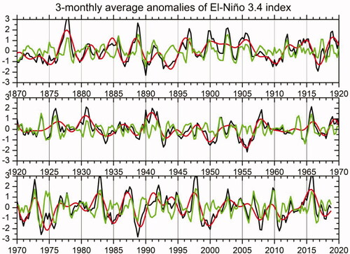
Fig. 1. Detrended and standardized time series in the period 1870–2018, of the three-monthly average anomalies (with respect to the annual cycle) of El Niño 3.4 index (black) and its low-pass (red) and high-pass (green) components with a cutoff frequency of 0.08 cycles per trimester roughly corresponding, respectively, to inter- and intra-triennial timescales variability.

3. Autocorrelation and spectrum

3.1. Autocorrelation function

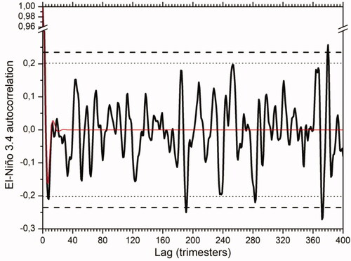
We start by evaluating second-order lagged moments of the time series. The autocorrelation function $C_x\left(\tau \right)\equiv \frac{1}{N-\tau }{\sum }_{t=0}^{N-\tau -1}x\left(t\right)x\left(t+\tau \right)\mathrm{ }$ is shown in Fig. 2. It has oscillatory behaviour with typical ENSO timescales (3–4 years). In order to test the null hypothesis $H_0$ of a vanishing autocorrelation, taking into account the serial correlation, we use an approximate effective sample size $N_{\mathit{eff}}\approx \frac{N\left[1-C_x\left(1\right)\right]}{\left[1+C_x\left(1\right)\right]}\approx 66$ (Wilks, 2011). Then, $H_0\mathrm{ }$ is rejected if ${\left|C_x\right(\tau \left)\right|}^2>[q_{\frac{\alpha }{2}}(N_{\mathit{eff}}{)]}^2/\left\{\right[q_{\frac{\alpha }{2}}(N_{\mathit{eff}}{)]}^2+N_{\mathit{eff}}-2\}$ (von Storch and Zwiers, 1999) where $q_{\frac{\alpha }{2}}\left(N_{\mathit{eff}}\right)$ is the $\frac{\alpha }{2}$-th quantile of a t-Student PDF with $N_{\mathit{eff}}$ degrees of freedom. From Fig. 2, some local extremes and significant correlations appear also at decadal lags.

Fig. 2. Autocorrelation function of El Niño 3.4 index (solid black) along with the 95% (dashed black) and 90% (dotted black) confidence interval. The autocorrelation function of the AR(5) model fitting data is also shown (solid red).

3.2. The spectrum and its estimation

A regularly sampled stationary time-series $x\left(t\right)$ can be decomposed using discrete Fourier transform (DFT) as: $X_x(f)={\sum }_{t=0}^{N-1}x\left(t\right)\hspace{0.17em}\text{exp}\hspace{0.17em}(-2\pi \mathit{ift}),$ for every frequency $f$ in cycles per sampling period and can be reconstructed through the inverse Fourier transform (FT) as $x(t)=\frac{1}{N}{\sum }_{K=-\frac{N}{2}}^{\frac{N}{2}}{X}_x\left(\frac{k}{N}\right)\hspace{0.17em}\text{exp}\hspace{0.17em}(2\pi i\frac{k}{N}t)$ (for $N$ even). The sample spectrum or periodogram is the DFT of the autovariance function: (1) $$S_x\left(f\right)=\frac{1}{N}{\left|X_x\left(f\right)\right|}^2={\sum }_{\tau =-\left(N-1\right)}^{N-1}{C}_x\left(\tau \right)\hspace{0.17em}\text{exp}\hspace{0.17em}(-2\mathit{\text{πifτ}})\ge 0$$(1) whereas the asymptotic spectrum is given by: (2) $${\Gamma }_x\left(f\right)=\underset{N\to \mathrm{\infty }}{\mathit{lim}}E\left[S_x\right(f\left)\right]$$(2)

where $E(·)$ is the expectation operator over realizations of the stochastic process. According to the Wiener–Khintchine theorem (2(2) $${\Gamma }_x\left(f\right)=\underset{N\to \mathrm{\infty }}{\mathit{lim}}E\left[S_x\right(f\left)\right]$$(2) ) is the FT of the autocovariance function i.e.: (3) $${\gamma }_x\left(\tau \right)={\int }_{-\frac{1}{2}}^{\frac{1}{2}}{\Gamma }_x\left(f\right)\hspace{0.17em}\text{exp}\hspace{0.17em}(2\mathit{\text{πifτ}})df.$$(3)

Equation (3)(3) $${\gamma }_x\left(\tau \right)={\int }_{-\frac{1}{2}}^{\frac{1}{2}}{\Gamma }_x\left(f\right)\hspace{0.17em}\text{exp}\hspace{0.17em}(2\mathit{\text{πifτ}})df.$$(3) yields, in particular, the variance of the time series (4) $${\gamma }_x\left(0\right)={\int }_{-\frac{1}{2}}^{\frac{1}{2}}{\Gamma }_x\left(f\right)df\approx \frac{1}{N}[S_x\left(0\right)+2{\sum }_{k=1}^{\frac{N}{2}}{S}_x\left(\frac{k}{N}\right)],$$(4) where ${\mathrm{\Gamma }}_x(f)df$ in (4(4) $${\gamma }_x\left(0\right)={\int }_{-\frac{1}{2}}^{\frac{1}{2}}{\Gamma }_x\left(f\right)df\approx \frac{1}{N}[S_x\left(0\right)+2{\sum }_{k=1}^{\frac{N}{2}}{S}_x\left(\frac{k}{N}\right)],$$(4) ) provides the contribution from the spectrum to the time series variance within the frequency interval $\left[f,f+df\right].$

For a stationary process, the DFTs $X_x(f),$ estimated at different frequencies are nearly uncorrelated (von Storch and Zwiers, 1999), and the periodogram (1(1) $$S_x\left(f\right)=\frac{1}{N}{\left|X_x\left(f\right)\right|}^2={\sum }_{\tau =-\left(N-1\right)}^{N-1}{C}_x\left(\tau \right)\hspace{0.17em}\text{exp}\hspace{0.17em}(-2\mathit{\text{πifτ}})\ge 0$$(1) ), is known to be inconsistent, and hence a smoothed estimator is often used: (5) $${\widehat{S}}_x(f)=\sum _{\tau =-\left(N-1\right)}^{N-1}{C}_x\left(\tau \right)\lambda \left(\tau \right)\hspace{0.17em}\text{exp}\hspace{0.17em}(-2\mathit{\text{πifτ}})$$(5) where $\lambda \left(\tau \right)\equiv \widehat{\lambda }\left(\frac{\tau }{M}\right)$ where $\widehat{\lambda }(·)$ is a symmetric standardized positive lag window function (Priestley, 1981), characterized by a standardized bandwidth $b_1\equiv \frac{1}{{\int }_{-\mathrm{\infty }}^{\mathrm{\infty }}{\widehat{\lambda }\left(u\right)}^{2}du}.$ The window scale length $M$ is chosen, based on a trade-off between spectral resolution ${(b}_1/M),$ low values of the variance $(\mathit{var}[{\widehat{S}}_x(f)]\sim \left[\frac{{{\mathrm{\Gamma }}_x\left(f\right)}^{2}M}{N{b}_1}\right])$ and bias $(E[{\widehat{S}}_x\left(f\right)]-{\mathrm{\Gamma }}_x(f)\sim \frac{-{\widehat{\lambda }}^{\text{″}}\left(0\right){{\mathrm{\Gamma }}_x^{\text{″}}\left(f\right)}^{}}{4{\pi }^2{M}^2})$ of (5) (Jenkins and Watts, 1968), where double apostrophe represents second derivatives. The 90% confidence interval of ${\mathrm{\Gamma }}_x\left(f\right)$ is given by $\left[\frac{\mathrm{ }{\widehat{S}}_x(f)\nu }{q_{95\mathrm{\%}}\left({\chi }_{\nu }^2\right)},\frac{\mathrm{ }{\widehat{S}}_x(f)\nu }{q_{5\mathrm{\%}}\left({\chi }_{\nu }^2\right)}\right],$ where $\nu =\frac{2N{b}_1}{M}\mathrm{ }$ is the number of degrees of freedom of the ${\chi }_{\nu }^2.$

We have also computed, the maximum entropy estimator of the spectrum by fitting an autoregressive (AR) model of generic order $p,$ via the Yule–Walker equations. The order is chosen by minimizing the Akaike Information Criterion, AIC (Akaike, 1974). The goal of computing the theoretical maximum entropy spectrum is to build a null hypothesis spectrum ${\mathrm{\Gamma }}_{x,0}\left(f\right).$ Therefore, in order to objectively check if the spectral peaks of (1) and (5) are truly distinguishable and significantly larger than those of ${\mathrm{\Gamma }}_{x,0}\left(f\right),\mathrm{ }$ at a significance level $\alpha ,$ the estimated spectra (1,5) have to be compared to the threshold $\frac{{\mathrm{\Gamma }}_{x,0}\left(f\right)q_{1-\alpha }\left({\chi }_{\nu }^2\right)}{\nu }$ (Wilks, 2011) with $\nu =\frac{2N{b}_1}{M}$ for (5) and $\nu =1$ for (1) corresponding to $M=N,$ and a standardized bandwidth equal to the Nyquist frequency.

3.3. El Niño index spectrum

3.3.1. Periodogram and smoothed spectrum

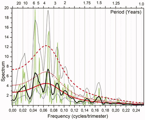
The periodogram (1(1) $$S_x\left(f\right)=\frac{1}{N}{\left|X_x\left(f\right)\right|}^2={\sum }_{\tau =-\left(N-1\right)}^{N-1}{C}_x\left(\tau \right)\hspace{0.17em}\text{exp}\hspace{0.17em}(-2\mathit{\text{πifτ}})\ge 0$$(1) ) of the time series is shown in Fig. 3. There is evidence of sharp and well separated peaks near the frequencies 0.021, 0.045, 0.071, 0.087, 0.105, and 0.168 cycles per trimester (cpt), corresponding (in the same order) to periods of 12.2 years, linked to decadal variability (Sun and Yu, 2009; Kravtsov, 2012), 5.62 years (Kim, 2002), and 3.53, 2.87, 2.38 and 1.49 years in the range of the ‘Quasi-quadrennial and quasi-biennial variability’ (Jiang et al., 1995). These peaks are also found by Deser et al. (2010) that are responsible for variations in the ENSO frequency, intensity, propagation, and predictability (e.g., An and Wang, 2000; Fedorov and Philander, 2000; Timmermann, 2003; An and Jin, 2004; Yeh and Kirtman, 2004; Wang, 2018).

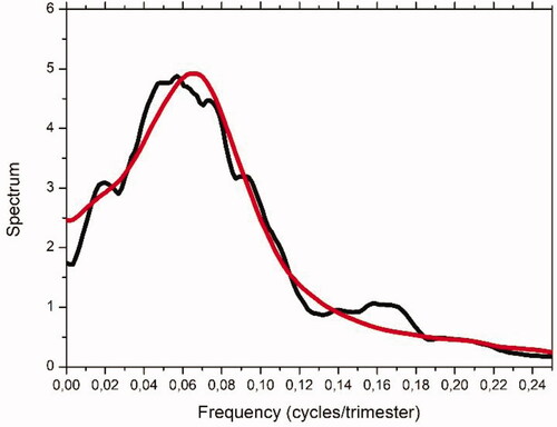
Fig. 3. Empirical periodogram (thin green); Smoothed spectrum (thick black) and corresponding 95% confidence interval (thin black); theoretical AR(5) spectrum (red), and 10% significance level for the periodogram (red dashed) and for the smoothed spectrum (red dotted). Units are (°C)²/cpt. The top axis presents periods in years.

For the smoothed spectrum (5(5) $${\widehat{S}}_x(f)=\sum _{\tau =-\left(N-1\right)}^{N-1}{C}_x\left(\tau \right)\lambda \left(\tau \right)\hspace{0.17em}\text{exp}\hspace{0.17em}(-2\mathit{\text{πifτ}})$$(5) ), we chose the Bartlett–Priestley window-lag function: $\widehat{\lambda }\left(u\right)=\frac{3}{(\pi u{)}^2}\left[\frac{\hspace{0.17em}\text{sin}\hspace{0.17em}(\pi u)}{\pi u}-\hspace{0.17em}\text{cos}\hspace{0.17em}(\pi u)\right]\text{}\left(u\ne 0\right);\widehat{\lambda }\left(0\right)=1$ (Priestley, 1981) for which$\mathrm{ }{b}_1$=0.855 and ${\widehat{\lambda }}^{\text{″}}\left(0\right)=-1.97.$ In order to resolve the main spectral peaks, the bandwidth $\frac{b_1}{M}\mathrm{ }$ must be smaller than the minimum difference between consecutive leading frequencies, i.e. $\frac{b_1}{M}<0.016\mathrm{ }$ cpt, hence $M>\frac{b_1}{0.016}\sim 52$ trimesters. To further increase spectral resolution, we show in Fig. 3 the estimator (5) using $M=80\mathrm{ }$(20 years), corresponding to $\nu \sim 13.$ In this case, the standard deviation of the filtered estimator is about 39% of the true spectrum. The 90% confidence interval for ${\mathrm{\Gamma }}_x\left(f\right)$ is $\left[0.52{\widehat{S}}_x(f),2.62{\widehat{S}}_x(f)\right]$ which is quite large, a consequence of the high window length $M.$ The local maxima of the filtered estimator lie close to the high spikes. Moreover, the periodogram lies well within the 95% confidence interval of the true spectrum (see thin black lines of Fig. 3).

3.3.2. Maximum entropy spectrum

An AR(5) model (see the AIC in Table 1) is fitted here: (6) $$\begin{array}{c}\tilde{x}\left(t\right)=1.18\tilde{x}\left(t-1\right)-0.46\tilde{x}\left(t-2\right)-0.09\tilde{x}\left(t-3\right)\\ +0.17\tilde{x}\left(t-4\right)-0.12\tilde{x}\left(t-5\right)+0.524w\left(t\right),\end{array}$$(6) where $w\left(t\right)$ is a standard Gaussian white noise. The autocorrelation function of the AR(5) model (Fig. 2) closely captures the empirical one for lags up to 12–20 trm but misses low-frequency oscillations. The corresponding (theoretical) maximum entropy spectrum is shown in Fig. 3 showing a spectral bump in the range (3–5 years period) and with no other spectral peaks. Figure 3 also shows the thresholds of significance (at α = 10%) for the periodogram and for the smoothed spectrum.

Table 1. Values of the Akaike Information Criterium $\mathit{AIC}(p)=N\mathit{ln}(2\pi e{\sigma }_{w,p}^2)+2p,$ where ${\sigma }_{w,p}^2$ is the residual noise variance of an AR(p) model fitting.

$p$	0	1	2	3	4	5	6
$\mathit{AIC}(p)$	1691.4	1085.2	939.9	941.9	943.4	936.6	937.6

The peaks with periods 5.62, 3.53, and 1.49 years are significant, both in the periodogram (1(1) $$S_x\left(f\right)=\frac{1}{N}{\left|X_x\left(f\right)\right|}^2={\sum }_{\tau =-\left(N-1\right)}^{N-1}{C}_x\left(\tau \right)\hspace{0.17em}\text{exp}\hspace{0.17em}(-2\mathit{\text{πifτ}})\ge 0$$(1) ) and the smoothed spectrum (5(5) $${\widehat{S}}_x(f)=\sum _{\tau =-\left(N-1\right)}^{N-1}{C}_x\left(\tau \right)\lambda \left(\tau \right)\hspace{0.17em}\text{exp}\hspace{0.17em}(-2\mathit{\text{πifτ}})$$(5) ) whereas the peak 2.87 years is significant in the periodogram (1(1) $$S_x\left(f\right)=\frac{1}{N}{\left|X_x\left(f\right)\right|}^2={\sum }_{\tau =-\left(N-1\right)}^{N-1}{C}_x\left(\tau \right)\hspace{0.17em}\text{exp}\hspace{0.17em}(-2\mathit{\text{πifτ}})\ge 0$$(1) ) but only marginally significant in the smoothed spectrum (5(5) $${\widehat{S}}_x(f)=\sum _{\tau =-\left(N-1\right)}^{N-1}{C}_x\left(\tau \right)\lambda \left(\tau \right)\hspace{0.17em}\text{exp}\hspace{0.17em}(-2\mathit{\text{πifτ}})$$(5) ).

4. Bicovariance, non-Gaussianity and nonlinearity

4.1. General properties

The bicovariance function ${\gamma }_x\left({\tau }_1,{\tau }_2\right)$ is a generalization of the autocovariance function, given by third-order cumulants between lagged values of $x\left(t\right),$ which for a zero mean stationary process writes as ${\gamma }_x\left({\tau }_1,{\tau }_2\right)=E\left[x\left(t\right)x\left(t+{\tau }_1\right)x\left(t+{\tau }_2\right)\right]$ and is estimated here, for ${\tau }_1,{\tau }_2\ge 0$ as: (7) $$C_x\left({\tau }_1,{\tau }_2\right)=\frac{1}{N-\mathit{max}({\tau }_1,{\tau }_2)}\sum _{t=0}^{N-\mathit{max}({\tau }_1,{\tau }_2)-1}x\left(t\right)x\left(t+{\tau }_1\right)x\left(t+{\tau }_2\right).$$(7)

Stationarity implies time invariance of lagged statistics leading to several identities reflecting the symmetry of the bicovariance (Rao and Gabr, 1984), namely: (8) $$\begin{array}{c}{\gamma }_x\left({\tau }_1,{\tau }_2\right)={\gamma }_x\left({\tau }_2,{\tau }_1\right)={\gamma }_x\left(-{\tau }_1,{\tau }_2-{\tau }_1\right)={\gamma }_x\left(-{\tau }_2,{\tau }_1-{\tau }_2\right)={\gamma }_x\left({\tau }_2-{\tau }_1,-{\tau }_1\right)=\\ ={\gamma }_x\left({\tau }_1-{\tau }_2,-{\tau }_2\right)\end{array}$$(8) leading to the partition into 6 sectors of the plane $\left({\tau }_1,{\tau }_2\right)$ as illustrated in Fig. 4a. We stress here that the origin of a non-vanishing bicovariance is the non-Gaussianity of the process $x\left(t\right).$ In fact, for a Gaussian, (necessarily linear) process, the bicovariance vanishes because cumulants of order 3 (the equivalent to lagged skewness) or higher vanish. For finite time series, Gaussianity is rejected if the absolute value of skewness is large enough.

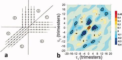
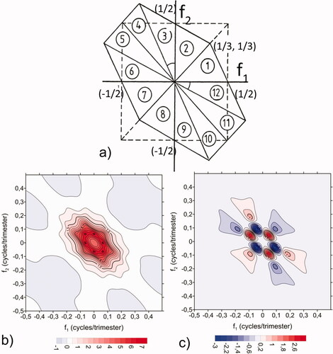
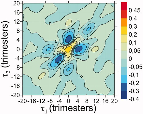
Fig. 4. Symmetries (a) of the bicovariance function in the delay plan (adapted from Rao and Gabr, 1984) and bicorrelation of El Niño 3.4 index (b). Thick black contours show the 5% significance level.

For a nonvanishing third-order cumulant, the bicorrelation provides a measure of predictability (for lags $\Delta \ge 0$), coming from nonlinear correlation: (9) $$\mathit{cor}\left[x\left(t+\Delta \right),x\left(t\right)x\left(t-{\tau }_1\right)\right]=\frac{C_x\left({\tau }_1,{\tau }_1+\Delta \right)}{\sqrt{\mathit{var}[x\left(t\right)x(t+{\tau }_1)]}}.$$(9)

Local maxima and minima of bicorrelation can thus provide sources of predictability due to non-Gaussianity and/or nonlinearity. However, we must note that part of the nonlinear correlation (9(9) $$\mathit{cor}\left[x\left(t+\Delta \right),x\left(t\right)x\left(t-{\tau }_1\right)\right]=\frac{C_x\left({\tau }_1,{\tau }_1+\Delta \right)}{\sqrt{\mathit{var}[x\left(t\right)x(t+{\tau }_1)]}}.$$(9) ), in particular at ${\tau }_1=0,$ is due to skewness, and hence to eliminate that contribution, we must consider the nonlinear component or residual $x_{nl}(t)=x(t{)}^2-[{sk}_x\mathrm{ }x\left(t\right)+1],$ of the predictor $x(t{)}^2$ after removing the linear regression with $x\left(t\right),$ where ${sk}_x\mathrm{ }$ is a regression constant equal to the skewness of $x.$

Another useful advantage of bicorrelation is the Cox (1991) test of nonlinearity, that we will apply bellow, also based on skewness. More general tests exist, which analyse nonlinear predictability originating from a set of past values (Granger and Anderson, 1978). Under the null hypothesis of linearity, the test $T_{\mathit{Cox}}(\Delta )\equiv \mathit{cor}[x(t+\Delta ),x_{nl}(t){]}^2$ must vanish for all lags. Threshold values of $T_{\mathit{Cox}}$ under an inexistent predictability hypothesis are obtained by randomly shuffling $x\left(t\right)$ and $x_{nl}\left(t\right)$ (10,000 times) and then computing the 95% quantile (denoted as $T_{\mathit{Cox}-95\mathrm{\%}}$) of the sorted values of $T_{\mathit{Cox}}\left(0\right).$ Nonlinearity of El Niño is thus accepted if $T_{\mathit{Cox}}\left(\Delta \right)>T_{\mathit{Cox}-95\mathrm{\%}}$ at a 5% significance level.

4.2. Results for El Niño index

4.2.1. Bicorrelation

The bicorrelation (Fig. 4b), exhibits fluctuations of the order of 12–20 trimesters similar to the autocorrelation (Fig. 2). The maximum value of the bicorrelation coincides with the skewness: $C_x\left(0,0\right)=0.46.$

In order to test the departure of the bicorrelation from the Gaussian hypothesis, we have generated 10,000, $N$-sized simulations with the AR(5) and computed uncertainties. The 90% (95%) quantiles of $\left|C_{\tilde{x}}\right(0,0\left)\right|\mathrm{ }$ are equal to 0.24 (0.29), which are both below the observed skewness 0.46, hence the null hypothesis of Gaussianity is rejected at the 5% significance level. For ${\tau }_1\sim {\tau }_2$ (diagonals of the bicovariance graph) or (${\tau }_1\sim 0\mathrm{ }$ and/or ${\tau }_2\sim 0$), the 95% (90%) quantiles are ∼0.14 (0.16) and 0.10 (0.12) elsewhere. The rejection regions rejecting of the null hypothesis (at the 5% significance level) appear within thick black contours in Fig. 4b.

From inspection of Fig. 4b, we verify that the deepest bicovariance minimum $C_x\left(0,4\right)=-0.40,$ is significant at the 5% significance level, corresponding to a nonlinear correlation (Eq. (9)(9) $$\mathit{cor}\left[x\left(t+\Delta \right),x\left(t\right)x\left(t-{\tau }_1\right)\right]=\frac{C_x\left({\tau }_1,{\tau }_1+\Delta \right)}{\sqrt{\mathit{var}[x\left(t\right)x(t+{\tau }_1)]}}.$$(9) ) of $\mathit{cor}[x(t+4),x(t{)}^2]=-0.24$ with ${\tau }_1=0,\Delta =4\mathrm{ }\mathit{trm}.$ This implies that an extreme El Niño or La Niña (high ${x(t)}^2$ than average) favours the occurrence of La Niña occurrence four trimesters later (negative $x\left(t+4\right)),$ whereas mild conditions favour El Niño. Another local bicorrelation minimum $C_x\left(8,8\right)=-0.15$ (10% significance level) implies that La Niña event favours a strong El Niño or La Niña 2 years later (8 trm).

4.2.2. Linear and nonlinear predictability

As regards El Niño predictability skill, Fig. 5a shows the linear and nonlinear correlations: $\mathit{cor}\left[x\left(t+\Delta \right),x\left(t\right)\right]$ and $\mathit{cor}\left[x\left(t+\Delta \right),x_{nl}\left(t\right)\right],$ with $x_{nl}\left(t\right)$ defined in Section 4.1 and for forecast lags $\Delta$ up to 20 trm. The linear correlations of El Niño 3.4 are significant at 10% level for lags $\Delta \le 3\mathrm{ }\mathit{trm}$ (Fig. 5a thick black line) whereas the nonlinear correlations show significant values for lags $3\mathrm{ }\mathit{trm}\le \Delta \le 5\mathrm{ }\mathit{trm}\mathrm{ }$(Fig. 5a thick red line). Those correlations are also evaluated for the stronger El Niño season i.e., the JFM trimester ($t+\Delta$ in JFM) (Fig. 5a thin black line for linear and thin red line for nonlinear correlations respectively). We note here the presence of the Spring predictability barrier of El Niño (Duan and Wei, 2013) i.e., the barely weak linear extrapolation (i.e. persistence) of El Niño index from current Spring (AMJ) to the next Winter (JFM), as shown by the small value (∼0.05) of $\mathit{cor}[x(t+\Delta ),x\left(t\right) | t+\Delta =\mathit{JFM}]$ where | means 'conditionated to' and $\Delta =3.$ However, the Spring barrier is reduced if we include the nonlinear term in the forecast. In fact, the nonlinear correlation evaluated at $\mathit{JFM}$ (Fig. 5a thin red line) for forecast lags $\Delta =3-5\mathrm{ }\mathit{trm}\mathrm{ }$(–0.25 to −0.4) is statistically significant, e.g. a negative value of $\mathit{cor}[x(t+3),{x\left(t\right)}^2 | t=\mathit{AMJ},\mathrm{ }t+3=\mathit{JFM}]$ between $x\left(t\right)$ in Spring and $x\left(t+3\right)$ in next Winter (see Fig. 5b).

Fig. 5. (a) Linear (thick black) and nonlinear (thick red) correlations ($\mathit{cor}\left[x\left(t+\Delta \right),x\left(t\right)\right]$ and $\mathit{cor}\left[x\left(t+\Delta \right),x_{nl}\left(t\right)\right]$ respectively) of El Niño 3.4 index. The same correlations restricted to forecast trimester JFM (black thin and red thin respectively). Horizontal dashed lines show the 10% significance level interval $\left[-\frac{1.64}{\sqrt{N_{\mathit{eff}}-3}},\frac{1.64}{\sqrt{N_{\mathit{eff}}-3}}\right].$ (b) AMJ versus following year JFM El Niño and best quadratic fitting. (c) Cox test $T_{\mathit{Cox}}\left(\Delta \right)$ (thick) and the 95% (dotted) and 99% (dashed) confidence level threshold of nonrejection of the linearity hypothesis.

This is corroborated by the conditional expectations of the Winter signal conditioned to the previous Spring signal. First, we have $E[x(t+3) |\mathrm{ }x\left(t\right)<-1]=-0.38$ (see left sector of Fig. 5b). We argue that strong trade-winds (or persistent eastern wind bursts in the Eastern Pacific), favouring strong La Niña Spring conditions tend to persist over some trimesters eventually reaching the next Winter season (e.g. JFM of years 1989, 1974, and 2011).

On the other hand, we have $E[x(t+3) |\mathrm{ }-1<x\left(t\right)<1]=0.12$ (central sector of Fig. 5b) corresponding to (Spring) near climatological conditions in the Eastern Pacific. Here, the tendency is to favour a Winter with El Niño predominance in agreement with Boreal Winter phase-locking. In particular, strong Winter El Niños (e.g. 1983, 1998, and 2016) were preceded by quite mild Spring conditions. Finally, from $E[x(t+3) | \mathrm{ }x\left(t\right)>1]=-0.19,$ strong El Niño Spring conditions (associated with westerly winds anomalies) tend to reverse in the next trimesters. This suggests that the nonlinear predictability is a consequence of the asymmetric persistence of El Niño signal and Pacific trade winds in Spring, as a function of their intensity and phase. A possible mechanism for this is seasonal growth rate dependence on the ENSO regime and feedbacks controlling SST (Yishuai et al., 2020), and the seasonal dependence of easterly wind bursts from Spring to Autumn (Fan et al., 2019).

Finally, we compute the nonlinear forecast score $T_{\mathit{Cox}}\left(\Delta \right)$ for lags up to 80 trm (Fig. 5c). Clearly, the nonlinearity is especially significant at certain lags (4–8, 28, 36, 52, 72, 80 trm) where $T_{\mathit{Cox}}\left(\Delta \right)$ is even larger than the quantile $T_{\mathit{Cox}-99\mathrm{\%}}$ of nonrejection of the linearity hypothesis. Those lags are related to phase synchronization between Fourier frequencies, namely those with periods ${\tau }_1$ and ${\tau }_2=2{\tau }_1.$ Lags are generally close to multiples of the half-period of the shorter oscillation, i.e. $\Delta =\frac{n{\tau }_1}{2},\mathrm{ }nϵ\mathbb{N}.$ For instance, from Fig. 3, the Fourier spectral peaks at periods ${\tau }_1=\frac{1}{0.087}=11.5\mathrm{ }\mathit{trm}$ and ${\tau }_2=\frac{1}{0.045}\approx 2{\tau }_1$ justify the peak of $T_{\mathit{Cox}}(\Delta )$ at lag $\Delta =\frac{5{\tau }_1}{2}\approx 29\mathrm{ }\mathit{trm}\mathrm{ }.$ This frequency relationship is known as quadratic phase coupling (Biswas et al., 1995) and examples in relation to decadal variability of ENSO are given in Timmermann (2003).

5. Bispectrum

5.1. General properties

5.1.1. Bispectrum background

The bicovariance of El Niño time series (Fig. 4b) exhibits certain features and periodicities in the lag-time domain. Therefore, the two-dimensional Fourier transform of the bicovariance, i.e. bispectrum (Brillinger and Rosenblatt, 1967), can provide a dual complementary information about the most relevant spectral interactions contributing to the bicovariance and skewness of the time series making easier the physical interpretation of such interactions.

The bispectrum is the two-dimensional version of polyspectra (Brillinger, 1965), providing relevant information on non-Gaussian processes. The bispectrum ${\Gamma }_{3,x}\left(f_1,f_2\right)\mathrm{ }$ is given by: (10) $${\Gamma }_{3,x}\left(f_1,f_2\right)\equiv \sum _{{\tau }_1=-\mathrm{\infty }}^{\mathrm{\infty }}\sum _{{\tau }_2=-\mathrm{\infty }}^{\mathrm{\infty }}{\gamma }_x\left({\tau }_1,{\tau }_2\right)\hspace{0.17em}\text{exp}\hspace{0.17em}[-2\pi i(f_1{\tau }_1+f_2{\tau }_2)],$$(10) where its real and imaginary parts are discrete Fourier transforms (DFT) of the symmetric and antisymmetric parts of the bicovariance, respectively, with the last one vanishing if the underlying stochastic process is reversible (Weiss, 1975).

For the simplest case of a purely random noise $w\left(t\right),$ the bicovariance is a spike at the origin i.e. ${\gamma }_w\left({\tau }_1,{\tau }_2\right)=E\left(w^3\right)\delta \left({\tau }_1\right)\delta \left({\tau }_2\right)$ where $\delta \left(·\right)$ is the Kronecker delta, yielding a flat, constant and real bispectrum ${\mathrm{\Gamma }}_{3,w}\left(f_1,f_2\right)=E\left(w^3\right).$

5.1.2. Bispectrum and spectral components

The asymptotic bispectrum of a N-sized time series writes in terms of DFTs $X_x\left(·\right)$ of the time series, taken at triplets of frequencies (multiples of the minimum frequency $\frac{1}{N}$) (Hinich, 1982) at $f_1,f_2$ and $f_3=\left[\left(f_1+f_2+\frac{1}{2}\right)mod\left(1\right)-\frac{1}{2}\right]$ as: (11) $${\Gamma }_{3,x}\left(f_1,f_2\right)=\underset{N\to \mathrm{\infty }}{\mathit{lim}}\frac{1}{N}E\left[X_x\left(f_1\right)X_x\left(f_2\right){X_x\left(f_3\right)}^{\mathrm{*}}\right]$$(11) where (*) stands for conjugate complex. Eq. (11)(11) $${\Gamma }_{3,x}\left(f_1,f_2\right)=\underset{N\to \mathrm{\infty }}{\mathit{lim}}\frac{1}{N}E\left[X_x\left(f_1\right)X_x\left(f_2\right){X_x\left(f_3\right)}^{\mathrm{*}}\right]$$(11) shows that the bispectrum comes from the interaction between Fourier components at three frequencies $f_1,f_2$ and $f_3=f_1+f_2<1/2$ in the area outside of the aliasing region, i.e. lower than the Nyquist frequency. When $f_1+f_2>1/2,$ then $f_3={1-(f}_1+f_2)$ becomes an aliased frequency (Hinich and Wolinsky, 1988).

Equation (11)(11) $${\Gamma }_{3,x}\left(f_1,f_2\right)=\underset{N\to \mathrm{\infty }}{\mathit{lim}}\frac{1}{N}E\left[X_x\left(f_1\right)X_x\left(f_2\right){X_x\left(f_3\right)}^{\mathrm{*}}\right]$$(11) can still be interpreted in terms of the amplitude and phase of the DFT in polar form, i.e. $X_x\left(f\right)\equiv {A_x(f)e}^{[i{\mathrm{\Theta }}_x(f)]\mathrm{ }}.$ By denoting $A_x\left(f_1\right)A_x\left(f_2\right)A_x\left(f_3\right)\equiv A_{x,123},\mathrm{ }$ and $e^{i\left[{\mathrm{\Theta }}_x\right(f_1)+{\mathrm{\Theta }}_x(f_2)-{\mathrm{\Theta }}_x(f_3\left)\right]}\equiv e^{i{\mathrm{\Theta }}_{x,123}},$ and applying the product expectation decomposition to (11), we get (Kovach et al., 2018): (12) $${\Gamma }_{3,x}\left(f_1,f_2\right)=\underset{N\to \mathrm{\infty }}{\mathit{lim}}\frac{1}{N}E\left[A_{x,123}\right]E\left[e^{i{\Theta }_{x,123}}\right]\mathrm{ }+\mathrm{ }\underset{N\to \mathrm{\infty }}{\mathit{lim}}\frac{1}{N}cov\left(A_{x,123},e^{i{\Theta }_{x,123}}\right),$$(12) where the first r.h.s. term of (12(12) $${\Gamma }_{3,x}\left(f_1,f_2\right)=\underset{N\to \mathrm{\infty }}{\mathit{lim}}\frac{1}{N}E\left[A_{x,123}\right]E\left[e^{i{\Theta }_{x,123}}\right]\mathrm{ }+\mathrm{ }\underset{N\to \mathrm{\infty }}{\mathit{lim}}\frac{1}{N}cov\left(A_{x,123},e^{i{\Theta }_{x,123}}\right),$$(12) ) depends on phase synchronization of the three Fourier components and the second term is a covariance between amplitudes and phases, vanishing for linear processes. In fact, the Volterra representation of a linear process writes as a convolution: $x\left(t\right)={\sum }_k^{}\alpha \left(k\right)w\left(t-k\right),$ where $w(t)$ is a purely random noise. Its DFT is $X_x\left(f\right)={X_{\alpha }\left(f\right)X_w\left(f\right)=X}_{\alpha }\left(f\right){A_w(f)e}^{[i{\mathrm{\Theta }}_w(f)]\mathrm{ }}$ where ${\mathrm{ }X}_{\alpha }\left(f\right),X_w\left(f\right)\mathrm{ }$ are DFTs, respectively of the sequence $\alpha \left(·\right)$ and of the noise. The independence between $A_w\left(f\right)$ and ${\mathrm{\Theta }}_w(f)$ yields ${\mathrm{\Gamma }}_{3,x}\left(f_1,f_2\right)={\mathrm{ }X}_{\alpha }\left(f_1\right){\mathrm{ }X}_{\alpha }\left(f_2\right){{\mathrm{ }X}_{\alpha }\left(f_3\right)}^{\mathrm{*}}\mathrm{ }E\left(w^3\right),\mathrm{ }$ restricted to the synchronization term (Nikias and Raghuveer, 1987), where$\mathrm{ }E\left(w^3\right)=\underset{N\to \mathrm{\infty }}{\mathit{lim}}\frac{1}{N}E\left[A_{w,123}\right]E\left[e^{i{\mathrm{\Theta }}_{w,123}}\right],$ showing hence the intrinsic nonlinear origin of the covariance term of (12).

5.1.3. Properties of the bispectrum

Like the spectrum, the bispectrum of a real signal satisfies ${\mathrm{\Gamma }}_{3,x}\left({-f}_1,{-f}_2\right)={{\mathrm{\Gamma }}_{3,x}\left(f_1,f_2\right)}^{\mathrm{*}},$ and (11(11) $${\Gamma }_{3,x}\left(f_1,f_2\right)=\underset{N\to \mathrm{\infty }}{\mathit{lim}}\frac{1}{N}E\left[X_x\left(f_1\right)X_x\left(f_2\right){X_x\left(f_3\right)}^{\mathrm{*}}\right]$$(11) ) leads to 5 identities of symmetry, namely: (13) $$\begin{array}{c}{\Gamma }_{3,x}\left(f_1,f_2\right)={\Gamma }_{3,x}\left(f_2,f_1\right)={\Gamma }_{3,x}\left(f_1,-f_1-f_2\right)={\Gamma }_{3,x}\left(-f_1-f_2,f_2\right)\\ ={\Gamma }_{3,x}\left(-f_1-f_2,f_1\right)={\Gamma }_{3,x}\left(f_2,-f_1-f_2\right).\end{array}$$(13)

This allows for a partition of the bispectrum domain (BD) into 12 polygonal regions in which the bispectrum can be reproduced from the Principal Domain (PD): the triangle of vertices (0,0), (0,1/2) and (1/3,1/3) (shown by triangle 1 in Fig. 6a). The periodicities are evident in the theoretical bispectrum in Fig. 6b (real part) and Fig. 6c (imaginary part) of a non-Gaussian AR(5) model of El Niño (presented later in Section 5.3.1).

Fig. 6. Principal domain (triangle 1) in the spectral plane and its symmetric replicas (a) (adapted from Rao and Gabr (1984). Real (b) and Imaginary (c) parts of the bispectrum of the NGAR(5) model. Note the symmetries associated with the 12 sectors shown in panel a).

The reconstruction of bicovariance is obtained through the inverse FT of (10): (14) $${\gamma }_x\left({\tau }_1,{\tau }_2\right)={\int }_{-\frac{1}{2}}^{\frac{1}{2}}{\int }_{-\frac{1}{2}}^{\frac{1}{2}}{\Gamma }_{3,x}\left(f_1,f_2\right)\hspace{0.17em}\text{exp}\hspace{0.17em}[2\pi i(f_1{\tau }_1+f_2{\tau }_2)]d{f}_{1}d{f}_2,$$(14) which leads to the skewness decomposition in terms of positive or negative contributions given by the real parts along the PD: (15) $$E\left(x^3\right)={\gamma }_x\left(0,0\right)=12{\iint }_{PD}\mathit{Re}[{\Gamma }_{3,x}(f_1,f_2)]d{f}_{1}d{f}_{2.}$$(15)

It is important to note here that, like the power spectrum (4(4) $${\gamma }_x\left(0\right)={\int }_{-\frac{1}{2}}^{\frac{1}{2}}{\Gamma }_x\left(f\right)df\approx \frac{1}{N}[S_x\left(0\right)+2{\sum }_{k=1}^{\frac{N}{2}}{S}_x\left(\frac{k}{N}\right)],$$(4) ), (15(15) $$E\left(x^3\right)={\gamma }_x\left(0,0\right)=12{\iint }_{PD}\mathit{Re}[{\Gamma }_{3,x}(f_1,f_2)]d{f}_{1}d{f}_{2.}$$(15) ) implies that the element of the bispectrum $\mathit{Re}[{\mathrm{\Gamma }}_{3,x}(f_1,f_2)]d{f}_{1}d{f}_2$ provides the contribution to the skewness $E\left(x^3\right)$ from the bi-spectral bin $\left[f_1,f_1+d{f}_1\right]\times [f_2,f_2+d{f}_2].$

Finally, since the square correlation is a predictability measure coming from third-order moments (see Eq. (9)(9) $$\mathit{cor}\left[x\left(t+\Delta \right),x\left(t\right)x\left(t-{\tau }_1\right)\right]=\frac{C_x\left({\tau }_1,{\tau }_1+\Delta \right)}{\sqrt{\mathit{var}[x\left(t\right)x(t+{\tau }_1)]}}.$$(9) ), its overall sum can be distributed over the bispectral domain through the Parseval relationship: (16) $${\sum }_{{\tau }_1}^{}{\sum }_{{\tau }_2}^{}[{\gamma }_x({\tau }_1,{\tau }_2){]}^2={\int }_{-\frac{1}{2}}^{\frac{1}{2}}{\int }_{-\frac{1}{2}}^{\frac{1}{2}}\left|{\Gamma }_{3,x}\right(f_1,f_2){|}^{2}d{f}_{1}d{f}_2=12{\iint }_{PD}\left|{\Gamma }_{3,x}\right(f_1,f_2){|}^{2}d{f}_{1}d{f}_2.$$(16)

5.2. Bispectrum estimation

The estimation of bispectrum has been addressed by many authors (e.g. Brillinger and Rosenblatt, 1967; Raghuvver and Nikias, 1986; Nikias and Raghuveer, 1987). The empirical bispectrum or biperiodogram of a finite sample of length $N$ is the two-dimensional DFT of the sampled bicovariance, which can also be expressed in terms of DFTs of the signal (see Section 3.1): (17) $$S_{3,x}\left(f_1,f_2\right)\equiv \sum _{{\tau }_1=-\left(N-1\right)}^{N-1}\sum _{{\tau }_2=-\left(N-1\right)}^N{C}_x\left({\tau }_1,{\tau }_2\right)\hspace{0.17em}\text{exp}\hspace{0.17em}[-2\pi i(f_1{\tau }_1+f_2{\tau }_2)]=\frac{1}{N}{X}_x(f_1\left)X_x\right(f_2){X_x\left(f_3\right)}^{\mathrm{*}}$$(17) where $f_3=\left(f_1+f_2+\frac{1}{2}\right)mod\left(1\right)-\frac{1}{2}.$ The inverse FT of Eq. (17)(17) $$S_{3,x}\left(f_1,f_2\right)\equiv \sum _{{\tau }_1=-\left(N-1\right)}^{N-1}\sum _{{\tau }_2=-\left(N-1\right)}^N{C}_x\left({\tau }_1,{\tau }_2\right)\hspace{0.17em}\text{exp}\hspace{0.17em}[-2\pi i(f_1{\tau }_1+f_2{\tau }_2)]=\frac{1}{N}{X}_x(f_1\left)X_x\right(f_2){X_x\left(f_3\right)}^{\mathrm{*}}$$(17) yields the empirical bicovariance: (18) $$C_x\left({\tau }_1,{\tau }_2\right)=\frac{1}{N^2}\sum _{k_1=-\frac{N}{2}}^{\frac{N}{2}}\sum _{k_2=-\frac{N}{2}}^{\frac{N}{2}}{S}_{3,x}\left(\frac{k_1}{N},\frac{k_2}{N}\right)\hspace{0.17em}\text{exp}\hspace{0.17em}[2\pi i(\frac{k_1}{\mathrm{N}}{\tau }_1+\frac{k_2}{N}{\tau }_2)]$$(18)

Like the periodogram (1(1) $$S_x\left(f\right)=\frac{1}{N}{\left|X_x\left(f\right)\right|}^2={\sum }_{\tau =-\left(N-1\right)}^{N-1}{C}_x\left(\tau \right)\hspace{0.17em}\text{exp}\hspace{0.17em}(-2\mathit{\text{πifτ}})\ge 0$$(1) ), the estimator (17(17) $$S_{3,x}\left(f_1,f_2\right)\equiv \sum _{{\tau }_1=-\left(N-1\right)}^{N-1}\sum _{{\tau }_2=-\left(N-1\right)}^N{C}_x\left({\tau }_1,{\tau }_2\right)\hspace{0.17em}\text{exp}\hspace{0.17em}[-2\pi i(f_1{\tau }_1+f_2{\tau }_2)]=\frac{1}{N}{X}_x(f_1\left)X_x\right(f_2){X_x\left(f_3\right)}^{\mathrm{*}}$$(17) ) is not consistent, which can be overcome by (i) smoothing the sample bispectrum (Hinich, 1982) or dividing the sample into pieces and then averaging and smoothing bispectra (Lii and Rosenblatt, 1982); (ii) using multi-tapers (Birkelund and Hanssen, 1999, 2000) or (iii) smoothing the bicovariance function (indirect-method) (Rao and Gabr, 1984), which we use here.

The smoothed bispectrum is: (19) $${\widehat{S}}_{3,x}(f_1,f_2)=\sum _{{\tau }_1=-N}^N\sum _{{\tau }_2=-N}^N{C}_x\left({\tau }_1,{\tau }_2\right)\Lambda \left({\tau }_1,{\tau }_2\right)\hspace{0.17em}\text{exp}\hspace{0.17em}[-2\pi i(f_1{\tau }_1+f_2{\tau }_2)]$$(19) where the 2D-lag window $\mathrm{\Lambda }(·)$ satisfies similar properties of symmetry as the bicovariance (8) and is taken to be $\mathrm{\Lambda }\left({\tau }_1,{\tau }_2\right)=\widehat{\lambda }\left(\frac{{\tau }_1}{M_2}\right)\widehat{\lambda }\left(\frac{{\tau }_2}{M_2}\right)\widehat{\lambda }\left(\frac{{\tau }_1}{M_2}-\frac{{\tau }_2}{M_2}\right)$ where $\widehat{\lambda }(\mathrm{ })\mathrm{ }$ is the lag window function and $M_2$ is the window length. The equivalent to bandwidth is given by $\frac{b_2}{M_2^2}$ where $b_2=1/{\int }_{-\mathrm{\infty }}^{-\mathrm{\infty }}{\int }_{-\mathrm{\infty }}^{\mathrm{\infty }}{\left[\widehat{\lambda }\left(u\right)\widehat{\lambda }\left(v\right)\widehat{\lambda }\left(u-v\right)\right]}^{2}du\mathrm{ }dv=1.19$ (Appendix A).

5.3. Bispectrum estimation of El Niño index

5.3.1. Null hypothesis bispectrum

To reproduce the observed skewness, we can construct an AR process driven by a non-Gaussian noise as a null hypothesis$\mathrm{ }{H}_0.$

The model we wish to fit is like model (6(6) $$\begin{array}{c}\tilde{x}\left(t\right)=1.18\tilde{x}\left(t-1\right)-0.46\tilde{x}\left(t-2\right)-0.09\tilde{x}\left(t-3\right)\\ +0.17\tilde{x}\left(t-4\right)-0.12\tilde{x}\left(t-5\right)+0.524w\left(t\right),\end{array}$$(6) ) $\tilde{x}\left(t\right)={\sum }_{\tau =1}^{p}a\left(k\right)\tilde{x}\left(t-k\right)+{\sigma }_{w}w\left(t\right),$ but with a non-Gaussian $w\left(t\right)$ white noise, ${\sigma }_w^2=\frac{E\left(x^2\right)}{{\int }_{-\frac{1}{2}}^{\frac{1}{2}}{\left|A\left(f\right)\right|}^{-2}df}$ and $A\left(f\right)=1-{\sum }_{\tau =1}^{p}a\left(k\right)e^{\left(-2\mathit{\text{πiτf}}\right)}.$ The bispectrum of such a linear process (Nikias and Raghuveer, 1987) is: (20) $${\Gamma }_{3,\tilde{x}}\left(f_1,f_2\right)=\frac{{\sigma }_w^{3}E\left(w^3\right)}{A\left(f_1\right)A\left(f_2\right){A\left(f_1+f_2\right)}^{\mathrm{*}}},$$(20) with: (21) $$E\left(w^3\right)=\frac{E\left(x^3\right)}{{\sigma }_w^3{\int }_{-\frac{1}{2}}^{\frac{1}{2}}{\int }_{-\frac{1}{2}}^{\frac{1}{2}}{\left[A\left(f_1\right)A\left(f_2\right){A\left(f_3\right)}^{\mathrm{*}}\right]}^{-1}d{f}_{1}d{f}_2}$$(21)

By using the coefficients of the AR(5) model (6(6) $$\begin{array}{c}\tilde{x}\left(t\right)=1.18\tilde{x}\left(t-1\right)-0.46\tilde{x}\left(t-2\right)-0.09\tilde{x}\left(t-3\right)\\ +0.17\tilde{x}\left(t-4\right)-0.12\tilde{x}\left(t-5\right)+0.524w\left(t\right),\end{array}$$(6) ), we get the approximations ${\sigma }_w^2=0.275$ and $E\left(w^3\right)=0.895,$ hence ${\sigma }_w^{3}E\left(w^3\right)=0.129.$ This null $H_0$ is hereafter designated NGAR(5).

Figure 6 shows (Fig. 6b) and imaginary (Fig. 6c) parts of the bispectrum (20) of the NGAR(5) model over the global bifrequency domain. The real part is mostly positive whereas the imaginary part is formed by dipolar structures. Both parts reflect the symmetry shown in (13) and exhibit a positive band of maximum absolute values in the region near $f_1+f_2\sim 0.09\mathrm{ }$ cpt and $f_1,f_2\in [0.02,0.08]$ cpt, coinciding with the frequency range where the power of the AR(5) model (6) exceeds 3 (°C)²/cpt as seen in Fig. 3.

5.3.2. Empirical smoothed bispectrum

To estimate the empirical bispectrum using the smoothed estimator (19), we start by identifying the ideal window function $M_2,$ according to (A4) in Appendix A. The values of the bispectral fluctuations ${\sigma }_{{\widehat{s}}_{3,x}}$ and the average confidence interval half-size (cihs) of the bispectrum (given by the square root of the l.h.s. of (A4)) are given in Table 2 for several values of $M_2.$ In order to separate peaks, the condition ${\sigma }_{{\widehat{s}}_{3,x}}>\mathit{cihs}$ must be satisfied. As expected, smaller bandwidths (larger $M_2$) lead to larger bispectral fluctuations and larger bispectrum estimation errors via cish. From Table 2, the largest $M_2$ around which ${\sigma }_{{\widehat{s}}_{3,x}}>\mathit{cihs}$ is $M_2\sim 30,$ which is used below.

Table 2. Average fluctuations ${\sigma }_{{\widehat{s}}_{3,x}}$ of the bispectrum and the average confidence interval half-size (CIHS) for several values of the window length $M_2$ (Eq. (A4)(A4) $$>({{\Phi }_{1-\frac{\alpha }{2}})}^2\frac{M_2^2}{N{b}_2}\overline{{\Gamma }_x\left(f_1\right){\Gamma }_x\left(f_2\right){\Gamma }_x\left(f_3\right)}={\mathit{cish}}^2$$(A4) ).

$M_2$	10	20	30	40	80
${\sigma }_{{\widehat{s}}_{3,x}}$	1.16	1.67	2.00	2.27	3.69
CIHS	0.70	1.37	2.09	2.79	5.59

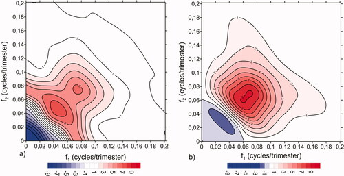
Figure 7 shows the real (Fig. 7a) and imaginary (Fig. 7b) parts of the smoothed bispectrum of the 3.4 El Niño index for the most relevant part of the first quadrant.

Fig. 7. Real (a) and Imaginary (b) part of the empirical bispectrum using a window lag (M₂ =30). Squared amplitude of the smoothed bispectrum (c). In figures a–c, significant regions at 20% significance level (or lower) appear within thick contours. Real (d) and imaginary (e) parts of the standardized bispectrum deviation $T_{x,\tilde{x}}\left(f_1,f_2\right)$ of El Niño index, and corresponding sum of the squared real and imaginary parts (f). Bifrequencies for which the null hypothesis $H_0$ is rejected at 20% significance levels (or lower) are color-shaded ($\left|T_{x,\tilde{x}})\right| >1.3$ for each part). Values are restricted to the most significant part of bispectrum.

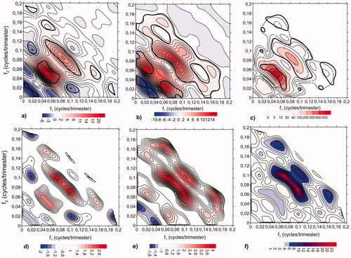
Both parts show several peaks. In particular, both present high absolute values for $f_1,\mathrm{ }{f}_2\in \left[0.04,0.07\right]\mathrm{ }$ cpt, as for null NGAR(5) model (Fig. 6) but with much larger amplitude. As expected, the average diameter of peaks is of the order of $\frac{\sqrt{b_2}}{M_2}=0.036\mathrm{ }\mathit{cpt}.$ The integral of $Re({\widehat{S}}_{3,x}$) (Fig. 7a) is the estimated skewness as Eq. (15)(15) $$E\left(x^3\right)={\gamma }_x\left(0,0\right)=12{\iint }_{PD}\mathit{Re}[{\Gamma }_{3,x}(f_1,f_2)]d{f}_{1}d{f}_{2.}$$(15) . According to Eq. (11)(11) $${\Gamma }_{3,x}\left(f_1,f_2\right)=\underset{N\to \mathrm{\infty }}{\mathit{lim}}\frac{1}{N}E\left[X_x\left(f_1\right)X_x\left(f_2\right){X_x\left(f_3\right)}^{\mathrm{*}}\right]$$(11) , the superposition of Fourier components along the triplet of frequencies $f_1,f_2,\mathrm{ }{f}_3=f_1+f_2$ where $Re()\mathrm{ }$ is positive (negative), will mostly generate extreme positive (negative) values, i.e. El Niño (La Niña) events. The integral of positive and negative values of $Re({\widehat{\mathrm{S}}}_{3,x}$) over the frequency domain is 0.54 and −0.08 respectively (adding up to the observed skewness 0.46). The local maxima of the real part, mostly contributing to El Niño extremes, lie near the frequency triplet ${(f}_1=f_2=0.05,\mathrm{ }{f}_3=0.1\mathrm{ }\mathit{cpt})$ and the band $({f_1+f_2=f}_3=0.165\mathrm{ }\mathit{cpt}),$ corresponding to local maxima of the power spectrum (Fig. 3), (e.g. quadratic phase synchronization Jajcay et al., 2018). On the other hand, the local minima of the real part, mostly contributing to La Niña extremes, lie near the frequency triplets ${(f}_1=f_2=0.018,\mathrm{ }{f}_3=0.036\mathrm{ }\mathit{cpt})$ and ${(f}_1=0.05,\mathrm{ }{f}_2=0.018,\mathrm{ }{f}_3=0.063\mathrm{ }\mathit{cpt}),$ which are again close to relative power maxima (see Fig. 3).

Figure 7c shows the squared bispectrum amplitude, providing the bispectral contribution to the predictability through (16), which agree quite well with Timmermann (2003). Its maxima occur near the local extremes of the real or imaginary parts of ${\widehat{S}}_{3,x}$ (Fig. 7a,b). The most relevant region for nonlinear predictability occurs for frequencies satisfying $f_1+f_2\in [0.07,\mathrm{ }0.1]$ cpt. Another maximum is observed for $f_1+f_2\in [0.16,\mathrm{ }0.18]$ cpt, producing oscillations with periods of 5–6 trimesters, and suggests possible source of the high nonlinear predictability for lags 5–6 trm, as diagnosed by Cox test in Fig. 5c.

5.3.3. Bispectrum and bicovariance near the origin

The bispectrum is relevant for the bicovariance behaviour near the origin. In fact, ${\gamma }_x\left({\tau }_1,{\tau }_2\right)$ can be approximated by a Taylor expansion: (22) $$\begin{array}{c}{\gamma }_x\left({\tau }_1,{\tau }_2\right)={\gamma }_x\left(0,0\right)+\sum _{p=1,2}\frac{\partial {\gamma }_x}{\partial {\tau }_p}{\tau }_p+\frac{1}{2}\sum _{p,q=1,2}\frac{{\partial }^2{\gamma }_x}{\partial {\tau }_p\partial {\tau }_q}{\tau }_p{\tau }_q\\ +\frac{1}{6}\sum _{p,q,r=1,2}\frac{{\partial }^3{\gamma }_x}{\partial {\tau }_p\partial {\tau }_q\partial {\tau }_r}{\tau }_p{\tau }_q{\tau }_r+O\left({\tau }_1^a{\tau }_2^b\right);\mathrm{ }a+b=4\end{array}$$(22) where derivatives are computed at ${\tau }_1={\tau }_2=0.$ Using Eq. (14)(14) $${\gamma }_x\left({\tau }_1,{\tau }_2\right)={\int }_{-\frac{1}{2}}^{\frac{1}{2}}{\int }_{-\frac{1}{2}}^{\frac{1}{2}}{\Gamma }_{3,x}\left(f_1,f_2\right)\hspace{0.17em}\text{exp}\hspace{0.17em}[2\pi i(f_1{\tau }_1+f_2{\tau }_2)]d{f}_{1}d{f}_2,$$(14) , we get: (23) $$\frac{\partial {\gamma }_x}{\partial {\tau }_p}=-{\iint }_{BD}\mathit{Im}[{\Gamma }_{3,x}(f_1,f_2)]2\pi f_{p}d{f}_{1}d{f}_2$$(23) (24) $$\frac{{\partial }^2{\gamma }_x}{\partial {\tau }_p\partial {\tau }_q}=-{\iint }_{BD}\mathit{Re}[{\Gamma }_{3,x}(f_1,f_2)]{\left(2\pi \right)}^2{f}_p{f}_{q}d{f}_{1}d{f}_2$$(24) (25) $$\frac{{\partial }^3{\gamma }_x}{\partial {\tau }_p\partial {\tau }_q\partial {\tau }_r}={\iint }_{BD}\mathit{Im}[{\Gamma }_{3,x}(f_1,f_2)]{\left(2\pi \right)}^3{f}_p{f}_q{f}_{r}d{f}_{1}d{f}_2.$$(25) where bicovariance symmetries lead to symmetries at the origin: $\frac{\partial {\gamma }_x}{\partial {\tau }_{\mathrm{p}}}=0,$ i.e. a local bicovariance extreme (see Fig. 4b) and $\frac{{\partial }^2{\gamma }_x}{\partial {\tau }_1\partial {\tau }_1}=\frac{{\partial }^2{\gamma }_x}{\partial {\tau }_2\partial {\tau }_2},\mathrm{ }\frac{{\partial }^3{\gamma }_x}{\partial {\tau }_1\partial {\tau }_1\partial {\tau }_1}=\frac{{\partial }^3{\gamma }_x}{\partial {\tau }_2\partial {\tau }_2\partial {\tau }_2},\frac{{\partial }^3{\gamma }_x}{\partial {\tau }_1\partial {\tau }_1\partial {\tau }_2}=\frac{{\partial }^3{\gamma }_x}{\partial {\tau }_2\partial {\tau }_2\partial {\tau }_1}.$

The partial derivatives at the origin, estimated with the smoothed El Niño bispectrum yield $\frac{{\partial }^2{C}_x}{\partial {\tau }_p\partial {\tau }_p}=-0.264\mathrm{ }\left(p=1,2\right),\mathrm{ }$ which explains most of the symmetric decrease of $C_x{(\tau }_1,{\tau }_2)$ near the origin (see Fig. 4b). The term $\frac{{\partial }^3{C}_x}{\partial {\tau }_p\partial {\tau }_p\partial {\tau }_p}=-0.114,$ however explains the asymmetry of that decrease, which is stronger for positive than negative lags yielding the bicovariance minimum $C_x\left(0,4\right)=-0.4.$

5.3.4. Bispectrum from frequency-band partitions

A coarse-grained description of the bispectrum can be achieved by classifying the triplets $f_1,f_2,f_3=f_1+f_2$ into sets of frequencies forming a partition of $[0,1/2].$ Each triplet is then characterized by the number of frequencies in each set. We consider the simple partition of the frequency interval using a cutoff frequency 0<$f_{\mathit{cut}}$<1/2, separating low (S) and high (F) frequencies, with the corresponding decomposition $x\left(t\right)=s\left(t\right)+f(t)$ (see Fig. 1). Figure 8a shows the 4 obtained subdomains namely, SSS, SSF, SFF and FFF, yielding an expansion into 4 terms of third-order statistics, e.g., (26) $$E\left(x^3\right)=E\left(s^3\right)+3E\left(s^{2}f\right)+3E\left({sf}^2\right)+E\left(f^3\right)=\mathit{SSS}+\mathit{SSF}+\mathit{SFF}+\mathit{FFF},$$(26)

Fig. 8. (a) Subdomains SSS, SSF, SFF and FFF obtained from a frequency partition using a cut-off frequency $f_{\mathit{cut}}=0.08$ cpt (∼3 years). (b) Contributing terms to El Niño 3.4 index skewness (Eq. (26)(26) $$E\left(x^3\right)=E\left(s^3\right)+3E\left(s^{2}f\right)+3E\left({sf}^2\right)+E\left(f^3\right)=\mathit{SSS}+\mathit{SSF}+\mathit{SFF}+\mathit{FFF},$$(26) ).

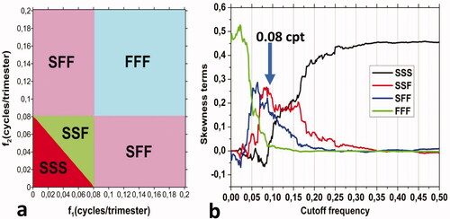
Figure 8b shows the terms in the r.h.s. of Eq. (26)(26) $$E\left(x^3\right)=E\left(s^3\right)+3E\left(s^{2}f\right)+3E\left({sf}^2\right)+E\left(f^3\right)=\mathit{SSS}+\mathit{SSF}+\mathit{SFF}+\mathit{FFF},$$(26) as a function of $f_{\mathit{cut}}.$ A reasonable criterion of discrimination among the different components is to choose $f_{\mathit{cut}}\mathrm{ }$ that maximizes the sum $\left|\mathit{SSS}\right|+\left|\mathit{SSF}\right|+\left|\mathit{SFF}\right|+|\mathit{FFF}$|, which takes place at $f_{\mathit{cut}}=0.082\mathrm{ }\mathit{cpt}$ (3.04 years). This yields inter- (slow S) and intra-triennial (fast F) variations with respective 82% and 38% explained variance, with a well-marked scale separation lying at a local minimum of the smoothed power spectrum (see Fig. 3), and a minimum value of $E\left(s^3\right)\mathrm{ }$(–0.066).

To see the impact of spectral decomposition on the different terms of skewness, we compare in Table 3 the terms of Eq. (26)(26) $$E\left(x^3\right)=E\left(s^3\right)+3E\left(s^{2}f\right)+3E\left({sf}^2\right)+E\left(f^3\right)=\mathit{SSS}+\mathit{SSF}+\mathit{SFF}+\mathit{FFF},$$(26) , derived directly from the time series to those obtained from the partial integrals of the smoothed bispectrum (Fig. 7a). Table 3 shows that the values are quite close, except for the negative value of $E\left(s^3\right).$ The underestimation obtained from the smoothed bispectrum is suggested to be due to the weak resolution of low frequencies.

Table 3. Contributing terms to skewness, Eq. (26)(26) $$E\left(x^3\right)=E\left(s^3\right)+3E\left(s^{2}f\right)+3E\left({sf}^2\right)+E\left(f^3\right)=\mathit{SSS}+\mathit{SSF}+\mathit{SFF}+\mathit{FFF},$$(26) , obtained from time series and from partial integrals of the smoothed bispectrum: total, negative and positive contributions. The most relevant integral positive (negative) contributions are marked in bold, representing the most relevant types of interaction contributing to extreme El Niño (La Niña) events.

	$\mathit{SSS}$	$\mathit{SSF}$	$\mathit{SFF}$	$\mathit{FFF}$
Time series	–0.066	0.263	0.185	0.071
$Re({\widehat{S}}_{3,x})$	–0.023	0.216	0.212	0.052
$Re\left({\widehat{S}}_{3,x}\right)<0$	–0.037	0.000	–0.031	–0.012
$Re\left({\widehat{S}}_{3,x}\right)>0$	0.014	0.216	0.243	0.063

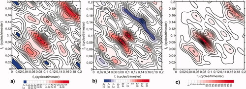
Extremes are classified according to the dominant term (SSS, SSF, SFF or FFF). From Table 3, extreme events of La Niña must be explained by the slow component $s\left(t\right)$ (e.g. 1887, 1917, 1956, 2000) or by phase synchronization of $s\left(t\right)\mathrm{ }$ and $f\left(t\right)$ (mostly of SFF type, e.g. 1973, 1988, 2008, and 2011) (Fig. 1). On the other hand, extreme events of El Niño, are mainly due to slow-fast component interactions, namely of SSF type (e.g. 1877, 1918, 1930, 1958, 2015) and SFF type (e.g. 1926, 1951, 1965, 1972, 1982–83, 1992, 1997, 2002) or from fast components only (FFF type) (e.g. 1923, 1977, 2006, 2009). However, some El Niño events (e.g. 1905, 1940, 1986–87), have occurred due to long persistence of the slow component (SSS type) (Fig. 1). Note also that there are few cases of phase polarity between fast and slow components (e.g. 1974) that lead to weak El Niño index.

In order to determine temporal changes of the bispectrum, we assess the third moment and its decomposition, Eq. (26)(26) $$E\left(x^3\right)=E\left(s^3\right)+3E\left(s^{2}f\right)+3E\left({sf}^2\right)+E\left(f^3\right)=\mathit{SSS}+\mathit{SSF}+\mathit{SFF}+\mathit{FFF},$$(26) , both in the full period (FULL) and along the three half-centuries: 1870–1919 (HC1), 1920–1969 (HC2 and 1970–2018 (HC3) (Fig. 1). Moreover, we evaluate the above statistics during El Niños $(x(t)>0)$ and La Niñas $(x(t)<0)$ to examine the variability of extremes and corresponding spectral contributions. For a given term in Eq. (26)(26) $$E\left(x^3\right)=E\left(s^3\right)+3E\left(s^{2}f\right)+3E\left({sf}^2\right)+E\left(f^3\right)=\mathit{SSS}+\mathit{SSF}+\mathit{SFF}+\mathit{FFF},$$(26) , for instance, SSS, its average $E\left(\mathit{SSS}\right)$ decomposes as: $E\left(\mathit{SSS}\right)={E(\mathit{SSS})}_{+}+{E(\mathit{SSS})}_{-},$ where ${E\left(\mathit{SSS}\right)}_{+}=E(\mathit{SSS}\mathit{ }\mathit{ }|\mathit{ }x>0\left)p\mathit{rob}\right(x>0)$ and ${E\left(\mathit{SSS}\right)}_{-}=E(\mathit{SSS}\mathit{ }\mathit{ }|\mathit{ }\mathit{ }x\le 0\left)p\mathit{rob}\right(x\le 0),$ giving the contributions to $E\left(\mathit{SSS}\right)$ during El Niños and La Niñas, respectively. Table 4 summarizes the results.

Table 4. Expected values (yellow) of the third moment of the normalized El Niño 3.4 index (denoted as sk) and its contributions SSS, SSF, SFF and FFF, as detailed in Eq. (26)(26) $$E\left(x^3\right)=E\left(s^3\right)+3E\left(s^{2}f\right)+3E\left({sf}^2\right)+E\left(f^3\right)=\mathit{SSS}+\mathit{SSF}+\mathit{SFF}+\mathit{FFF},$$(26) for the full period and for the three half centuries 1870–1919 (HC1), 1920–1969 (HC2) and 1970–2018 (HC3). The expectations and their bispectral contributions are further decomposed into contributions conditioned to La Niñas (blue) and conditioned to El Niños (red). Note that $sk={sk}_{+}+{sk}_{-}$ (idem for skewness terms).

	sk	SSS	SSF	SFF	FFF	sk–	SSS–	SSF–	SFF–	FFF–	sk+	SSS+	SSF+	SFF+	FFF+
FULL	0.5	–0.1	0.2	0.2	0.1	–0.6	–0.4	0	–0.2	–0.1	1.1	0.3	0.2	0.4	0.2
HC1	0.7	0.1	0.2	0.3	0.1	–0.5	–0.3	0	–0.1	–0.1	1.2	0.4	0.2	0.4	0.2
HC2	0.2	0	0.1	0.3	0	–0.3	–0.2	0	–0.1	–0.1	0.5	0.2	0.1	0.4	0.1
HC3	0.5	–0.3	0.5	0.2	0.1	–1.0	–0.6	0.2	–0.4	–0.2	1.5	0.3	0.3	0.6	0.3

First, the most recent half century (HC3) has on average, the most extreme episodes of La Niña and El Niño, as observed from the high absolute values of ${sk}_{-}$ and ${sk}_{+}.$ The amplification of La Ninãs comes mostly from a clear increase of self-slow interaction SSS=–0.06 and cross interaction SFF=–0.4 whereas amplification of El Niños comes from the enhancement of the SFF term (0.6), as compared to the previous two half centuries. This suggests changes and decadal variability of the ENSO skewness, its bicovariance and bispectrum (Wu and Hsieh, 2003), associated to changes in the preferential Fourier phase couplings (Schulte et al., 2019). This was accompanied by an ENSO regime shift, near 1970 towards more nonlinearity (An and Wang, 2000; An and Jin, 2004; An, 2009).

5.3.5. Statistical significance of the empirical bispectrum

It is important to check the acceptance or rejection of the null bispectrum $H_0$ of NGAR(5) (Fig. 6b,c). The spectral method used here is based on a variation of the Hinich (1982) test of linearity. We anticipate that both the local (A6) and the integrated (A7) spectral-based tests of nonlinearity in the bi-frequency domain reject the null $H_0$ in consistency with the nonlinearity Cox test in the time domain (see Section 4.2.2) and hence other sources of non-Gaussianity (e.g. deterministic nonlinearity and multiplicative noise) shall be necessary. Furthermore, as shown in Appendix A the asymptotic bias (A2), variance (A3) as well as the asymptotic Gaussian PDF (Rao and Gabr, 1984) of the smoothed estimator are not good approximations because of the small number of degrees freedom ${(N}_{\mathit{eff}}=66)$ of the time series and hence cannot be used to test the null $H_0.$ This could be alleviated by using, e.g. a very long run of a climate model simulation. We use a Monte-Carlo strategy by computing the statistics of bispectrum by generating 10,000 surrogates of the NGAR(5) model forced by a noise prescribed by its first three moments. In order to easily obtain noise realizations, we consider noises produced by polynomial independent standard Gaussian noises, by relating the coefficients of monomial expectations to the imposed noise moments. For instance, the first trial noise: ${\sigma }_{w}w\left(t\right)=a{w}_1\left(t\right)+b\left[w_1^2\left(t\right)-1\right]$ where $w_1$ is a standard Gaussian white noise, leads to ${\sigma }_w^2=a^2+2b^2=0.275$ and ${\sigma }_w^{3}E\left(w^3\right)=8b^3+6a^{2}b=0.129,$ yielding $a=0.5122,$ and $b=0.0794,$ and its excess kurtosis is 1.073.

Here, we choose: ${\sigma }_{w}w\left(t\right)=a{w}_1\left(t\right)+b\left[w_2^2\left(t\right)-1\right]$ where $w_1,w_2$ are independent standard Gaussians with ${\sigma }_w^2=a^2+2b^2=0.275$ and ${\sigma }_w^{3}E\left(w^3\right)=8b^3=0.129,$ yielding $a=0.3840,$ and $b=0.2525$ and a excess kurtosis of 2.475. The results are quite robust to changes in the noise model. Other possible, though less practical, noises are generated by maximum entropy constrained by the four first moments (Pires et al., 2010). We then compute the Monte-Carlo ensemble average $E\left[{\widehat{S}}_{3,\tilde{x}}\right]$ and variance $\mathit{var}\left[{\widehat{S}}_{3,\tilde{x}}\right],$ of the real and imaginary parts of the smoothed bispectrum. Noise high-order moments (greater than 2) appear only to influence the high-order moments of the smoothed spectrum (e.g. skewness and kurtosis) which are not relevant for the linearity test devised here.

The deviation of El Niño smoothed bispectrum ${\widehat{S}}_{3,x}\left(f_1,f_2\right)$ (Fig. 7a,b) from that of NGAR(5) model is assessed by the test statistic (standardized deviation) (Eq. (A6)(A6) $$T_{x,\tilde{x}}\left(f_1,f_2\right)\equiv \frac{{\widehat{S}}_{3,x}\left(f_1,f_2\right)-E\left[{\widehat{S}}_{3,\tilde{x}}\right]}{{\left[\mathit{var}\right({\widehat{S}}_{3,\tilde{x}}\left)\right]}^{1/2} }$$(A6) ): $T_{x,\tilde{x}}\left(f_1,f_2\right)\equiv \frac{{\widehat{S}}_{3,x}\left(f_1,f_2\right)-E\left[{\widehat{S}}_{3,\tilde{x}}\right]}{{(\mathit{var}[{\widehat{S}}_{3,\tilde{x}}])}^{1/2}\mathrm{ }}.$ Under $H_0,$ its real and imaginary parts are approximately standard Gaussian. We also limited the tests to frequencies with higher bispectrum amplitude, roughly corresponding to $\left|f_1\right|,\left|f_2\right|<0.2\mathrm{ }$(as in Fig. 7a,c). Figure 7 shows the real (Fig. 7d) and imaginary (Fig. 7e) parts of $T_{x,\tilde{x}}\left(f_1,f_2\right)$ where significant regions (at $\alpha =20\mathrm{\%}$ significance level). are color-shaded. Fig. 7d shows that most peaks of $Re({\widehat{S}}_{3,x})$ (Fig. 7a) are significant. In particular, the low-frequency region (SSS type), producing La Niña events for $\left|f_1\right|,\left|f_2\right|,\left|f_3\right|<0.06$ cpt, is significant (i.e. rejecting $H_0$). The other positive and negative bispectrum extremes discussed in Section 5.3.2 are also significant at $\alpha =10$%. The imaginary part of the test (Fig. 7e) and the squared amplitude (Fig. 7f) are also highly significant in most of the relevant regions of the bispectrum with significance levels reaching 5%. The most significant region of nonlinear predictability holds approximately for $f_1+f_2\mathrm{ }$ within $\left[0.16,\mathrm{ }0.18\right]\mathrm{ }$ cpt where bispectrum is significant at $\alpha =5\mathrm{\%},$ producing oscillations with periods of the order 5–6 trimesters. This suggests a possible source of the high nonlinear predictability for lags 3–6 trm, as diagnosed by Cox test (Fig. 5c), and for the nonlinear curtailing of El Niño Spring barrier (see Fig. 5a).

The local test $T_{x,\tilde{x}}\left(f_1,f_2\right)\mathrm{ }$ computed on a frequency basis may lead, ambiguously, either to the rejection or to the acceptance of linearity, depending on $f_1,f_2$ (see Fig. 7d–e). This is suggested by the fact that finite N-sized samples generated by the non-Gaussian NGAR(5) model led to local frequency tests $T_{\tilde{x},\tilde{x}}\left(f_1,f_2\right)$ where linearity is falsely rejected (not shown). Therefore, in order to overcome this difficulty and enhance test robustness, we propose the integrated test of nonlinearity (A7) given by $T_{\mathit{int}\mathrm{ }x,\tilde{x}}\equiv \sum _{\left(f_1,f_2\right)\in L}{{\mathrm{ }|T}_{x,\tilde{x}}\left(f_1,f_2\right)|}^2$ over a representative lattice $L$ (Fig. A3). We found that nonlinearity cannot be rejected (at 5% level), thanks to the highly significant regions of El Niño bispectrum (Fig. 7d–e and 7a–c).

5.3.6. Normalized bispectrum and bicoherency

An independent test of linearity, beyond that of previous section and diagnostic of phase synchronization comes from the normalized bispectrum or bicoherence spectrum (Kim and Powers, 1979; Nikias and Raghuveer, 1987; Hinich and Wolinsky, 2005; Rao et al., 2012). It is obtained by prewhitening $x\left(t\right)$ to yield a non-Gaussian white noise $y\left(t\right),$ and reconstructed by inverse FT of $X_y\left(f\right)\equiv \frac{X_x\left(f\right)}{{\left[{\mathrm{\Gamma }}_x\left(f\right)\right]}^{\frac{1}{2}}}={\sqrt{N}e}^{i[{\mathrm{\Theta }}_x(f)]}.$ The test is then: (27) $${\Gamma }_{3,y}\left(f_1,f_2\right)\mathrm{ }\equiv \frac{{\Gamma }_{3,x}\left(f_1,f_2\right)}{{\left(\mathrm{ }{\mathrm{\Gamma }}_x\left(f_1\right){\Gamma }_x\left(f_2\right){\Gamma }_x\left(f_3\right)\right)}^{\frac{1}{2}}}$$(27)

We stress that the phases of $X_y\left(f\right)$ and $X_x\left(f\right)\mathrm{ }$ are the same (i.e. ${\mathrm{\Theta }}_x\left(f\right)$), leading to a nonvanishing correlation $\mathit{cor}\left(x,y\right)={\sigma }_x^{-1}{\int }_{-\frac{1}{2}}^{\frac{1}{2}}\sqrt{{\mathrm{ }\mathrm{\Gamma }}_x(f)}\mathrm{ }df.$

A linear process i.e. $x\left(t\right)={\sum }_k^{}\alpha \left(k\right)w\left(t-k\right)$ where $w$ is a white noise yields ${\mathrm{\Gamma }}_x\left(f\right)={\left|{\mathrm{ }X}_{\alpha }\right(f\left)\right|}^{2}E\left(w^2\right).$ By using the result of Section 5.1.2, the normalized bispectrum (27(27) $${\Gamma }_{3,y}\left(f_1,f_2\right)\mathrm{ }\equiv \frac{{\Gamma }_{3,x}\left(f_1,f_2\right)}{{\left(\mathrm{ }{\mathrm{\Gamma }}_x\left(f_1\right){\Gamma }_x\left(f_2\right){\Gamma }_x\left(f_3\right)\right)}^{\frac{1}{2}}}$$(27) ) becomes ${\mathrm{\Gamma }}_{3,y}\left(f_1,f_2\right)=sk\left(w\right)e^{i\left[{\mathrm{\Theta }}_{\alpha }\right(f_1)+{\mathrm{\Theta }}_{\alpha }(f_2)-{\mathrm{\Theta }}_{\alpha }(f_3\left)\right]}$ where ${\mathrm{\Theta }}_{\alpha }\left(·\right)$ is the phase of the DFT of sequence $\alpha \left(k\right).$ Therefore, the amplitude of ${\mathrm{\Gamma }}_{3,y}\mathrm{ }$ is uniform, i.e.$\mathrm{ }\left|{\mathrm{\Gamma }}_{3,y}\left(f_1,f_2\right)\right|=sk\left(w\right)$ which is precisely the Hinich (1982) null hypothesis of linearity.

In the case of El Niño, we get an estimated prewhitened non-Gaussian noise $y\left(t\right)$ by using the more reliable theoretical maximum entropy NGAR(5) spectrum for the normalization in (27), instead of the empirical smoothed spectrum. The lag correlation of the resulting noise $y\left(t\right)$ is very close to zero and thus can be considered a white noise. Its skewness is $0.282$ and the excess kurtosis is $0.531.$ The correlation with the signal $x\left(t\right)$ is quite high: 0.75, coming mainly from extreme events.

The smoothed normalized bispectrum, using the same window length ${M=M}_2=30,$ is hereby denoted ${\widehat{S}}_{3,y}.$ Significant peaks (at 20% significance level) of ${\widehat{S}}_{3,y},$ both of the real (Fig. 9a) and imaginary (Fig. 9b) parts are located nearly at the same bifrequencies as the non-normalized bispectrum ${\widehat{S}}_{3,x}$ (Fig. 7a,b) though peaks are attenuated by normalization and a new peak appears at higher frequencies $f_1=f_2=0.18$ (2.5 years), ${(f}_3=0.36)$ cpts (2.8 years). The squared bicoherency ${\left|{\widehat{S}}_{3,y}\right(f_1,f_2\left)\right|\mathrm{ }}^2$ (Fig. 9c) is clearly nonuniform, showing regions of nonacceptance of the null bispectrum of NGAR(5) and hence rejecting the linearity hypothesis.

Fig. 9. Real (a) and Imaginary (b) parts of the normalized smoothed bispectrum of El Niño index, (M₂=30) and its squared amplitude (c). Regions statistically significant at 20% level are colour-shaded.

6. Stochastic modelling

6.1. The method

6.1.1. The motivation

ENSO has been extensively studied to look for a deeper understanding of the underlying physics and complexity (see recent reviews of Chunzai, 2018; Timmermann et al., 2018 and references therein), improve predictability (see the review of Tang et al., 2018), as well as to get accurate statistics (e.g. pdf, extremes etc.). This was done through different dynamical models (physical-based deterministic models), statistical models (e.g. linear inverse modelling by Penland (1996) and Privalsky and Muzylev, 2013) and models based on machine learning (Dijkstra et al., 2019).

However, even complex models may exhibit biases of various statistics. The present top-down approach of fitting simple stochastic models to observations, attempts learn signal-noise relationships from models, enabling parametrizations of the nonlinear and complex effects of nonobserved variables and hence reproducing a set of relevant stochastic properties (e.g. spectrum, bispectrum).

A number of stochastic univariate models of ENSO have been fitted such as: smooth transition autoregressive (STAR) models (Hall et al., 2001; Ubilava and Helmers, 2013), autoregressive conditional heteroscedasticity type models (ARCH) (Ahn and Kim, 2005), and threshold AR models (De Gooijer, 2017). This section aims at fitting a minimal univariate stochastic model for El Niño 3.4. index driven by a multiplicative Gaussian delayed noise, able to reproduce the observed empirical spectrum, skewness and bispectrum as well as assess the impact it has on predictability, compared to benchmark linear models.

6.1.2. The model formulation

The models fitted here, belong to a class in which the simulated scalar state $\tilde{x}\left(t\right),\mathrm{ }$ at integer $t,$ is driven by a noise$\mathrm{ }u\left(t\right)={\sigma }_{w}w\left(t\right)$ where $w(t)$ is a standard Gaussian white noise and ${\sigma }_w$ is a positive constant. The simulated state $\tilde{x}\left(t\right)$ depends (through a function F) on: a) the simulated previous state values at $t<0,$ represented in delay coordinate (Takens et al., 1981) by $\tilde{\mathit{x}}\left(t-1\right)\equiv {[\dots \tilde{x}(t-2),\tilde{x}(t-1\left)\right]}^T;$ b) the previous noise values at $t<0:$ $\mathit{u}\left(t-1\right)\equiv {[\dots u(t-2),u(t-1\left)\right]}^T$ and c) a parameter vector $\mathit{\theta }.$ Throughout this section bold letters refer to vectors and italic to scalars. The model writes thus as: (28) $$\tilde{x}\left(t\right)=F\left[\tilde{\mathit{x}}\right(t-1),\mathrm{ }\mathit{u}(t-1),\mathrm{ }\mathit{\theta }]+ u\left(t\right)$$(28)

The model (28) will also be used in forecast mode, and the $\tau$-lag $\left(\tau \ge 1\right)\mathrm{ }$ forecast valid at time at $t,$ $x\left(t,\tau \right),$ is given by: (29) $$x\left(t,\tau \right)=F\left[\mathit{x}\right(t-1,\tau -1),\mathrm{ }\mathit{ϵ}(t-1,\tau ),\mathrm{ }\mathit{\theta }],$$(29) where $\mathit{x}\left(t-1,\tau -1\right)\equiv {[\dots ,x(t-2,\tau -2),x(t-1,\tau -1\left)\right]}^T,$ with $x\left(t\mathrm{\prime },\tau \right)=x\left(t\mathrm{\prime }\right)$ for $\tau \le 0.$ The noise vector in (29) becomes $\mathit{ϵ}\left(t-1,\tau \right)\equiv {[\dots ,\epsilon (t-2,\tau -1),\epsilon (t-1,\tau \left)\right]}^T$ with $\epsilon \left(t^{\mathrm{\prime }},\tau \mathrm{\prime }\right)\equiv x\left(t^{\mathrm{\prime }},\tau \mathrm{\prime }\mathrm{\prime }-1\right)-x\left(t^{\mathrm{\prime }},\tau \mathrm{\prime }\mathrm{\prime }\right),$ where ${\tau }^{\text{″}}=\max \left(1,{\tau }^{\mathrm{\prime }}\right).\mathrm{ }$ For instance the one-step forecast is $x\left(t,1\right)=F\left[\mathit{x}\right(t-1,0),\mathrm{ }\mathit{ϵ}(t-1,1),\mathrm{ }\mathit{\theta }]$ where $\mathit{x}\left(t-1,0\right)=\mathit{x}\left(t-1\right)\equiv {\left[\dots ,x\left(t-2\right),x\left(t-1\right)\right]}^T\mathrm{ }$ and $\mathit{ϵ}\left(t-1,1\right)=\mathit{ϵ}\left(t-1\right)={[\dots ,\epsilon (t-2),\epsilon (t-1\left)\right]}^T$ with $\epsilon \left(t^{\mathrm{\prime }}\right)\equiv x\left(t^{\mathrm{\prime }}\right)-x\left(t^{\mathrm{\prime }},1\right)$ is the one-step error forecasts, being thus consistent with (28).

The models of form (28(28) $$\tilde{x}\left(t\right)=F\left[\tilde{\mathit{x}}\right(t-1),\mathrm{ }\mathit{u}(t-1),\mathrm{ }\mathit{\theta }]+ u\left(t\right)$$(28) ) include AR linear models, fitted in Section 3.3.2. However, in order to reproduce nonlinear and non-Gaussian ENSO behaviour, we have considered bilinear models (Haggan and Oyetunji, 1980; Rao and Gabr, 1984; Rao 1981), which differ from AR processes by the addition to them of lagged bilinear (BL) terms, denoted ARBL(p₁, p₂): (30) $$\begin{array}{c}F\left[\tilde{\mathit{x}}\left(t-1\right), \mathit{u}\left(t-1\right), \mathit{\theta }\right]={\sum }_{k=1}^{p_1}{a}_k\tilde{x}\left(t-l_k\right)\\ +{\sum }_{k=1}^{p_2}{b}_k\tilde{x}\left(t-r_k\right)u\left(t-s_k\right)+\alpha ,\end{array}$$(30) characterized by its correlated-additive–multiplicative (CAM) noise (Usoro, 2015), where $l_k,\mathrm{ }{r}_k,s_k\ge 1$ are lags, with $\mathit{\theta }\equiv \left(a_1,\dots ,a_{p_1},b_1,\dots ,b_{p_2},\alpha \right).$ These models can produce non-Gaussian statistics and nonvanishing bicovariances and bispectra (Rao and Gabr, 1984). Note that the restricted case of lags $r_k=0,\mathrm{ }{s}_k=0$ (Monahan, 2020) are excluded from model of Eq. (30)(30) $$\begin{array}{c}F\left[\tilde{\mathit{x}}\left(t-1\right), \mathit{u}\left(t-1\right), \mathit{\theta }\right]={\sum }_{k=1}^{p_1}{a}_k\tilde{x}\left(t-l_k\right)\\ +{\sum }_{k=1}^{p_2}{b}_k\tilde{x}\left(t-r_k\right)u\left(t-s_k\right)+\alpha ,\end{array}$$(30) , to allow inverting $u\left(t\right)$ from past values for forecasting. Note also that the case $r_k>s_k$ leads to sub-diagonal bilinear models whereas the case $r_k\le s_k$ corresponds to diagonal/super-diagonal bilinear models. In the former case, for example, the intervening noise is independent of the most recent state whereas the latter case corresponds to nonlinear feedbacks, having in general nonvanishing time averages due to correlation between states and past noises. We stress that models (30(30) $$\begin{array}{c}F\left[\tilde{\mathit{x}}\left(t-1\right), \mathit{u}\left(t-1\right), \mathit{\theta }\right]={\sum }_{k=1}^{p_1}{a}_k\tilde{x}\left(t-l_k\right)\\ +{\sum }_{k=1}^{p_2}{b}_k\tilde{x}\left(t-r_k\right)u\left(t-s_k\right)+\alpha ,\end{array}$$(30) ) have a nonlinear Volterra development in terms of lagged noises, which in a certain way parametrizes nonlinearities which are not present in a deterministic form in function $F.$ However, other type of models could be fitted, e.g. adding quadratic terms in the deterministic forcing but which can lead to instabilities in simulations. Another difficulty with nonlinear deterministic part, is the very wide class of nonlinearity: which nonlinearity: if polynomial-what degree? However, we investigate it in another study.

6.1.3. Model fitting

In order to optimize predictability and reproduce data statistics, we apply a hybrid fitting algorithm that minimizes a cost function $J_{\mathit{hyb}}$ which is the weighted sum of the normalized one-step forecast residuals $J_{\mathit{fitt}}$ and the normalized squared distance between a set of observed and simulated statistics (average, autocovariance and bi-covariance) $J_{\mathit{stat}}:$ (31) $$J_{\mathit{hyb}}\left(\mathit{\theta }\right)=c_{\mathit{fitt}}{J}_{\mathit{fitt}}\left(\mathit{\theta }\right)+c_{\mathit{stat}}{J}_{\mathit{stat}}\left(\mathit{\theta },{\sigma }_w\left(\mathit{\theta }\right)\right)$$(31) where $c_{\mathit{fitt}}$ and $c_{\mathit{stat}}$ are positive weights and ${\sigma }_w\left(\mathit{\theta }\right)={\sigma }_x{\left(J_{\mathit{fitt}}\left(\mathit{\theta }\right)\right)}^{1/2}$ is the RMS of the forecast residuals for a model using parameters $\mathit{\theta }$ with ${\sigma }_x=1$ (observations are standardized).

The term $J_{\mathit{fitt}}\mathrm{ }$ is given by the one-step forecast error: (32) $$J_{\mathit{fitt}}\left(\mathit{\theta }\right)=\frac{1}{(N-N_{\gamma }){\sigma }_x^2}\sum _{t=N_{\gamma }}^{N-1}{\left[x\left(t\right)-F\left[\mathit{x}\right(t-1),\mathrm{ }\mathit{ϵ}(t-1),\mathrm{ }\mathit{\theta }]\right]}^2$$(32) where $N_{\gamma }\equiv {\mathit{max}}_{k,k\mathrm{\prime }}(l_k,r_{k\mathrm{\prime }},s_{k\mathrm{\prime }}).$

Iterative minimization algorithms of $J_{\mathit{fitt}}\left(\mathit{\theta }\right)$ for general bilinear models are discussed in Pham and Tran (1981), (Rao and Gabr 1984), Grahn 1995, Guegan and Pham (1989), Gabr 1998 and Falguerolles and Francis (1992). Traditionally, the method of moments is used to obtain implicit relationships between the parameters and lagged moments (e.g. Sesay and Rao, 1988; Tang and Mohler, 1988; Kim et al., 1990), where, in most cases parameters are difficult to be expressed as a function of moments. Here we apply a method where statistics are estimated from a long simulation of (Eq. (28)(28) $$\tilde{x}\left(t\right)=F\left[\tilde{\mathit{x}}\right(t-1),\mathrm{ }\mathit{u}(t-1),\mathrm{ }\mathit{\theta }]+ u\left(t\right)$$(28) ) with initial conditions: $\tilde{x}\left(t\right)=w\left(t\right)=0;\mathrm{ }t=-N_{\mathit{past}},\dots ,{-N}_{\mathit{past}}+N_{\gamma },$ and $w\left(t\right)\sim N\left(0,1\right);t={-N}_{\mathit{past}}+N_{\gamma }+1,$…,$\mathrm{ }{N}_{\mathit{sim}}.$ Statistics are computed for $t=1,\dots ,N_{\mathit{sim}}$ with $N_{\mathit{sim}}=30,000$ and the initial $N_{\mathit{past}}=1000$ values are discarded from statistics as spin-up.

The term $J_{\mathit{stat}},$ involving the mean, autocovariance and bicovariance from observations, ($S_{\mathit{obs}},C_{\mathit{obs}}\left(·\right),$ and $B_{\mathit{obs}}\left(·,·\right)$), and simulations ($S_{\mathit{sim}},$ $C_{\mathit{sim}}\left(·\right),\mathrm{ }$ and $B_{\mathit{sim}}\left(·,·\right)),$ is (33) $$J_{\mathit{stat}}\left(\mathit{\theta },{\sigma }_w\right)=J_S\left(\mathit{\theta },{\sigma }_w\right)+J_C\left(\mathit{\theta },{\sigma }_w\right)+J_B\left(\mathit{\theta },{\sigma }_w\right),$$(33) where (34) $$\begin{array}{c}{J}_S\left(\mathit{\theta },{\sigma }_w\right)=\frac{{\left(S_{\mathit{sim}}-S_{\mathit{obs}}\right)}^2}{{\sigma }_x^2}\\ J_C\left(\mathit{\theta },{\sigma }_w\right)=\sum _{\left|\mathit{\tau }\right|\le {\tau }_{\mathit{max}}}^{}{\left[C_{\mathit{sim}}\left(\tau \right)-C_{\mathit{obs}}\left(\tau \right)\right]}^2\frac{b_1{\lambda \left(\tau \right)}^2}{{\tau }_{\mathit{max}}{\sigma }_x^4\mathrm{ }}\mathrm{ }\end{array}$$(34) (35) $$\sim \frac{b_1}{{\tau }_{\mathit{max}}{\sigma }_x^4\mathrm{ }}{\int }_{-1/2}^{1/2}{{\left[{{\widehat{S}}_{2,\tilde{x}}\left(f\right)-\widehat{S}}_{2,x}\left(f\right)\right]}^{2}df,}^{}$$(35) and (36) $$\begin{array}{c}{J}_B\left(\mathit{\theta },{\sigma }_w\right)\sum _{\left|{\tau }_1\right|,\left|{\tau }_2\right|\le {\tau }_{\mathit{max}}}{\left[B_{\mathit{sim}}\left({\tau }_1,{\tau }_2\right){-B}_{\mathit{obs}}\left({\tau }_1,{\tau }_2\right)\right]}^2\frac{b_2{\lambda \left({\tau }_1,{\tau }_2\right)}^2}{{\tau }_{\mathit{max}}^2{\sigma }_x^6\mathrm{ }}\\ \sim \frac{b_2}{{\tau }_{\mathit{max}}^2{\sigma }_x^6\mathrm{ }}{\int }_{-1/2}^{1/2}{\int }_{-1/2}^{1/2}{{\left[{\widehat{S}}_{3,\tilde{x}}\left(f_1,f_2\right){-\widehat{S}}_{3,x}\left(f_1,f_2\right)\right]}^2{df}_1{df}_2,}^{}\end{array}$$(36) with ${\tau }_{\mathit{max}}=16.$

The used window lag functions $\lambda (\tau )$ and $\lambda ({\tau }_1,{\tau }_2)$ are scaled by ${M=M_2=\tau }_{\mathit{max}}.$ The Parseval Theorem applied to (35–36), shows that minimizing $J_C\left(\mathit{\theta },{\sigma }_w\right),$ $J_B\left(\mathit{\theta },{\sigma }_w\right)$ leads also to minimizing errors in the spectral domain.

In the analysis we compare two situations: $c_{\mathit{fitt}}=1,c_{\mathit{stat}}=0$ (simple fitting) and the hybrid fitting where $c_{\mathit{fitt}}=1;\mathrm{ }{c}_{\mathit{stat}}=\Delta J_{\mathit{fitt}}$/${\Delta J}_{\mathit{stat}},$ given by the ratio of typical variations of $J_{\mathit{fitt}}$ and $J_{\mathit{stat}}$ (hybrid fitting). The optimal parameters issued from simple and hybrid fittings are hereby denoted ${\mathit{\theta }}_{\mathit{fitt}}$ and ${\mathit{\theta }}_{\mathit{hyb}},$ respectively. Note that the term $c_{\mathit{stat}}{J}_{\mathit{stat}}$ reduces overfitting and the domination of one term over the other, see Appendix B for the description of the minimization of $J_{\mathit{hyb}}\left(\mathit{\theta }\right).$ We compare both fittings in terms of $J_{\mathit{fitt}}$ and $J_{\mathit{stat}}$ for the AR(p₁) model and several ARBL(p₁, p₂) models. The statistical significance is given through the normalized Akaike Information Criterion: $\mathit{NAIC}=\log (J_{\mathit{fitt}})-2dim\mathit{\theta }/(N-N_{\gamma })$ that penalizes the number of model terms.

6.2. Results for El Niño index

6.2.1. Fitting statistics

We analyse and evaluate a sequence of models (Eq. (30)(30) $$\begin{array}{c}F\left[\tilde{\mathit{x}}\left(t-1\right), \mathit{u}\left(t-1\right), \mathit{\theta }\right]={\sum }_{k=1}^{p_1}{a}_k\tilde{x}\left(t-l_k\right)\\ +{\sum }_{k=1}^{p_2}{b}_k\tilde{x}\left(t-r_k\right)u\left(t-s_k\right)+\alpha ,\end{array}$$(30) ), for $p_1=5,$ $l_k=k;k=1,\dots ,p_1,$ with various $p_2$ values using lags $r_k\le 6,s_k\le 6$ (Table 5) with every new lag pair producing the largest $J_{\mathit{fitt}}$ decrease.

Table 5 shows that the mean residual squares $J_{\mathit{fitt}}\mathrm{ }$ decreases with increasing model complexity. For hybrid, NAIC decreases with increasing complexity (i.e., no overfitting). Moreover, the hybrid fitting is able to get improved statistics compared to that from the simple fitting ${(J}_{\mathit{stat}}\left({\mathit{\theta }}_{\mathit{hyb}}\right)<J_{\mathit{stat}}\left({\mathit{\theta }}_{\mathit{fitt}}\right)),$ with reductions up to about one fifth for the ARBL(5,5) model. That reduction entails very tiny increments in the sum of residuals$,\mathrm{ }$ i.e. $J_{\mathit{fitt}}\left({\mathit{\theta }}_{\mathit{hyb}}\right)>J_{\mathit{fitt}}\left({\mathit{\theta }}_{\mathit{fitt}}\right),$ of the order of 1%, but still keeping significant NAIC values.

Table 5. Statistics of the AR(5) and bilinear ARBL(5,1),…,ARBL(5,5) models with the corresponding bilinear-term lags ${(r}_{p_2},s_{p_2})\mathrm{ }$ along with the terms $J_{\mathit{fitt}}$ and $J_{\mathit{stat}}$ for simple and hybrid fitting in addition to the normalized AIC relative to hybrid fitting. Correlation skills ${\mathit{cor}}_{\tau }$ are also shown at lags $\tau =1,2,3$ trimesters, assessed over the period 1970–2018 for models obtained by hybrid fitting calibrated in the period 1870–1969.

Model	${(r}_{p_2},s_{p_2})$	$J_{\mathit{fitt}}(\mathit{simple})$	$J_{\mathit{stat}}\left(\mathit{simple}\right)$	$J_{\mathit{fitt}}(\mathit{hybrid})$	$J_{\mathit{stat}}\left(\mathit{hybrid}\right)$	$\mathit{NAIC}$	${\mathit{cor}}_1$	${\mathit{cor}}_2$	${\mathit{cor}}_3$
AR(5)		0.2779	0.0199	0.2784	0.0192	–1.268	0.855	0.552	0.261
ARBL(5,1)	(2,1)	0.2742	0.0211	0.2754	0.0145	–1.277	0.859	0.579	0.309
ARBL(5,2)	(2,4)	0.2708	0.0109	0.2738	0.0055	–1.282	0.864	0.607	0.379
ARBL(5,3)	(1,3)	0.2645	0.0138	0.2693	0.0062	–1.296	0.864	0.609	0.382
ARBL(5,4)	(6,3)	0.2601	0.0146	0.2639	0.0047	–1.315	0.865	0.598	0.333
ARBL(5,5)	(5,1)	0.2566	0.0151	0.2604	0.0034	–1.327	0.867	0.618	0.349

The estimated of the ARBL(5,5) model are shown in Table 6 and $\left(\alpha ,{\sigma }_w\right)=(0.0626,\mathrm{ }0.5102).$

Table 6. Coefficients and lags of the autoregressive and bilinear terms of the ARBL(5,5) model of El Niño index, obtained by hybrid fitting over the full period. The independent constant $\alpha =0.0626$ and the additive driving noise is $u\left(t\right)=0.5102 w\left(t\right).$

k	$a_k$	$b_k$	$({r_k,s}_k)$
1	1.130	0.289	(2,1)
2	–0.384	–0.154	(2,4)
3	–0.072	–0.114	(1,3)
4	0.159	0.100	(6,3)
5	–0.139	–0.108	(5,1)

6.2.2. Simulated autocovariance and spectrum

We note that the autoregressive part of the ARBL(5,5) model is quite similar to that of AR(5) model (Eq. (6)(6) $$\begin{array}{c}\tilde{x}\left(t\right)=1.18\tilde{x}\left(t-1\right)-0.46\tilde{x}\left(t-2\right)-0.09\tilde{x}\left(t-3\right)\\ +0.17\tilde{x}\left(t-4\right)-0.12\tilde{x}\left(t-5\right)+0.524w\left(t\right),\end{array}$$(6) ). The bilinear coefficients have smaller amplitude than the autoregressive coefficients. ARBL(5,5) contains two feedback terms corresponding to ${(r}_k,s_k)=(2,4\left)\text{ and }\right(1,3)$ whose nonzero mean values come from white noise squares and leading to a nonvanishing constant $\alpha .$ This parametrizes partially the bicovariance at the interseasonal scales which is at the origin of the nonlinear reduction of the Spring Predictability Barrier (see Section 4.2.2). The model recovers quite well the empirical autocovariance function (not shown), and also the smoothed spectrum (Fig. 10) using the window lag $M=30,$ with particularly similar peak in the band $f\sim 0.05-0.07$ cpt.

Fig. 10. Smoothed empirical (black) and ARBL(5,5) simulated (red) spectra using a window lag M = 30.

6.2.3. Simulated bicovariance and bispectrum

Most (∼80%) uncertainty in $J_{\mathit{hyb}}\left({\mathit{\theta }}_{\mathit{hyb}}\right)$ comes from the bicovariance uncertainty through $J_B\left(\mathit{\theta },{\sigma }_w\right).$ The simulated bicovariance (Fig. 11) reproduces very well the same pattern of the bicovariance inferred from observations (Fig. 4b), at least up to lags 12 trimesters. The simulation yields a skewness equal to 0.26, which is comparable with the observed skewness (0.46). Any simpler model with only one bilinear term is unable to yield positive skewness and negative bicovariances $C_{\tilde{x}}\left(0,3\right),\mathrm{ }{C}_{\tilde{x}}\left(0,4\right),$ which are fundamental to get skillful El Niño predictions from Spring to the next Winter.

Fig. 11. Bicorrelation of the ARBL(5,5) model, approaching the empirical bicorrelation of El Niño index (to be compared with Fig. 4b).

The smoothed bispectrum of the ARBL(5,5) simulation, using a window lag $M_2=30,$ is shown in Fig. 12a (real part) and Fig. 12b (imaginary part), to be compared with the empirical one (Fig. 7a,b). The real part (Fig. 7a) is quite well reproduced, with negative values in the low-frequency band $\left|f_1+f_2\right|<0.06,$ and positive local maxima near $f_1=f_2=0.045\mathrm{ }\mathit{cpts}\mathrm{ }$ and $f_1=f_2=0.085\mathrm{ }\mathit{cpts}$ (Fig. 12a). The decomposition of skewness (Eq. (26)(26) $$E\left(x^3\right)=E\left(s^3\right)+3E\left(s^{2}f\right)+3E\left({sf}^2\right)+E\left(f^3\right)=\mathit{SSS}+\mathit{SSF}+\mathit{SFF}+\mathit{FFF},$$(26) ), (with $f_{\mathit{cut}}=0.06$) yields the values −0.036, 0.062, 0.154 and 0.082 respectively for the SSS, SSF, SFF and SSS contributions, which agree approximately with observations (Table 3). The imaginary part of the simulated bispectrum (Fig. 12b) is also roughly well reproduced, showing negative values within the region $f_1+f_2<0.06$ (Fig. 7b) and positive elsewhere. The maximum is near $f_1=f_2\sim 0.07$ cpts. Note that the existence of a single peak is related to the simulated single-peak spectrum.

Fig. 12. Real (a) and Imaginary (b) parts of smoothed bispectrum of the ARBL(5,5) using a window lag M₂=30.

We shall remark that the bilinear models chosen here, have a linear deterministic part with nonlinearity coming indirectly through the CAM noise. However, other type of models could be fitted, e.g. adding quadratic terms in the deterministic forcing but which can lead to other difficulties like instabilities and chaotic behaviour in simulations.

6.2.4. Predictability

In order to assess the predictability impact of the inclusion of bilinear terms in ARBL models, compared to the AR(5) model, we compute the correlation skill ${\mathit{cor}}_{\tau },$ (Table 5) between observations and predictions for lags for $\tau =1,2,3$ trimesters. Models are optimized by hybrid fitting in the training period 1870–1969 (100 years) and predictions are evaluated in the validation period 1970–2018 (49 years), where the most intense La Niñas and El Niños have been observed (see Section 5.3.4). All the tested models’ predictions are skillful (${\mathit{cor}}_{\tau }$>0.5) for lags up to two trimesters.

Table 5 shows that, in general correlation skills increase with increasing complexity. For instance, the correlation skill of model ARBL(5,5) is about 2%, 7% and 9% larger than AR(5), respectively for lags of 1, 2 and 3 trimesters. The presence of at least two bilinear terms suggests the reason behind the improvement of the 2-trimester forecasts by ARBL(5,5), with respect to AR(5), for which some extreme El Niños (e.g. 1973, 1983, 1998, 2016) are more accurately predicted. The ARBL(5,5) model has no explicit deterministic nonlinearities, which are common to physically-based models. Here, nonlinearities are parametrized through the bilinear terms. Despite the simplicity of the ARBL(5,5) model, its correlation skills ${(\mathit{cor}}_1=0.87,\mathrm{ }{\mathit{cor}}_2=0.62)$ are not dramatically smaller, in the same period than those of physically-based models ${(\mathit{cor}}_1=0.85-0.91,\mathrm{ }{\mathit{cor}}_2=0.68-0.80)$ and to those of a much more complex neural-network based model ${(\mathit{cor}}_1=0.92,\mathrm{ }{\mathit{cor}}_2=0.80)$ as observed in Fig. 2a of (Ham et al., 2019).

7. Discussion and conclusion

El Niño Southern Oscillation (ENSO) is one of the most important coupled atmosphere–ocean system, exhibiting time scales ranging from seasons to decades and beyond, with a particularly worldwide teleconnection. Using different stochastic and/or dynamic approaches, most studies have emphasized and shown its intrinsic complexity, nonlinearity and non-Gaussianity. Most of those studies limited their investigations to the second order statistics in addition to skewness and/or kurtosis.

Here, we follow the same line of research by performing a data-driven systematic study of the third-order stochastic moments, both in the time and spectral domains, applied to the standardized trimonthly-average El Niño 3.4 index with a trimester sampling. Within the time domain, this comprises the bicovariance ${\gamma }_x\left({\tau }_1,{\tau }_2\right)=E\left[x\left(t\right)x\left(t+{\tau }_1\right)x\left(t+{\tau }_2\right)\right],$ in addition to nonlinear correlations for testing nonlinearity and nonlinear predictability for forecasting horizons from seasons up to a few years. The study uses a 149-year period (1870–2018) time series with its statistically significant skewness of 0.46, peaking mostly at the boreal winter (1.04). The analysis of bicovariance maxima reveals high negative nonlinear correlation, implying that El Niño or La Niña extremes are likely to be followed by La Niña one year later, whereas mild conditions, on the other hand, favour El Niño occurrence.

The analysis of the nonlinear predictability, on seasonal time scales, shows that such nonlinear correlation is enhanced further when forecasts are issued at the NH Spring season (AMJ). This is linked to the persistence of many La Niñas starting in Spring up to next Winter and to the fact that strong Winter El Niños have only occurred under close climatological conditions in the previous boreal Spring. This strongly suggests that nonlinearity in the inter-seasonal timescale can contribute significantly to reduce the so-called El Niño Spring predictability barrier. Another equally important aspect is the fact that ENSO nonlinearity allows for the extension of predictability skill even for forecasting time of a few years, particularly when these forecasting time intervals satisfy phase synchronization and quadratic phase locking with certain dominant Fourier frequencies.

Similarly, within the spectral domain the bispectrum and bicoherence have been computed. As with power spectrum and variance, the bispectrum provides, in particular, the contribution of each bi-frequency bin to the observed skewness and squared bicovariance. This warrants the detection of combinations of El Niño Fourier components that mostly contribute to ENSO extremes by phase synchronization. The bispectrum also permits a test of nonlinearity in the spectral domain. The bispectrum has been estimated by a smoothed estimator using a window lag of 30 trimesters = 7.5 years, obtained from a trade-off between bispectrum bias, variance, and spectral resolution. To estimate the statistical significance of peaks, a conservative test has been adopted. The bispectrum of a non-Gaussian autoregressive null-hypothesis model NGAR(5) is tested and rejected at 5% significance level. We first obtained the coarse-grained spectral partition of the skewness by splitting the full signal into a slow component $s\left(t\right)$ (with periods larger than 3 years) and a fast component $f\left(t\right).$ The skewness is then decomposed into 4 components, namely $\mathit{SSS}=-0.066,$ $\mathit{SSF}=0.263,$ $\mathit{SFF}=0.185\mathrm{ }$ and $\mathit{FFF}=0.071,$ implying, in particular, that most El Niños result from interaction between inter- and intra-triennial timescales. Some decadal tendency towards SFF-type El Niños is apparent from the time series, which is consistent with the observed ENSO decadal variability. Note that if a maximum of the bispectrum real part is observed at $(f_1,f_2)$ then a peak in the power spectrum is observed approximately at $f_3=f_1+f_2.$ In particular, the leading bispectral maxima contributing to El Niño occurs at $f_1=f_2=0.05,\mathrm{ }{f}_3=0.1\mathrm{ }\mathit{cpt}$ cpt (periods of 5 and 2.5 years inside the SSF region) and near the band $f_1+f_2=0.165\mathrm{ }\mathit{cpt},$ crossing the SFF and FFF regions, with a maximum at $f_1=f_2=0.082,\mathrm{ }{f}_3=0.165\mathrm{ }\mathit{cpt}$ (periods of 2.9 and 1.5 years). On the other hand, minima contributing mostly to La Niña extremes, lie near $f_1=f_2=0.018,\mathrm{ }{f}_3=0.036\mathrm{ }\mathit{cpt}\mathrm{ }$(periods of 14 and 7 years) and ${(f}_1,\mathrm{ }{f}_2)=(0.05,0.018),\mathrm{ }{f}_3=0.063\mathrm{ }\mathit{cpt}$ (periods of 5, 7 and 4 years), both inside the SSS region.

Lastly, a minimal stochastic model was constructed, which was able to reproduce the main features of the spectrum and bispectrum, and yielded robust improvement of the predictability skill, compared to an autoregressive AR(5) model. The model was selected from a large class of bilinear models with correlated-additive–multiplicative lagged noise. To gain predictability skill with the right stochastic properties, a hybrid fitting approach is used by minimizing a combination of forecasting squared residuals and squared deviations from empirical third-order statistics. The bilinear model yields forecast improvements, particularly at lags of 1, 2 and 3 trimesters with 2%, 7% and 9% of correlation skill increment respectively, suggested to be linked to the attenuation of El Niño predictability Spring barrier and to the more accurate prediction of super El Niños.

This study contributes to the understanding of ENSO predictability and modelling from the perspective of the bispectrum and phase synchronization. In a changing climate, this is especially relevant for the study and predictability of ENSO extremes resulting from resonant-type interaction. The study also provides the possibility to investigate other ENSO indices such as El-Nino Modoki or other Nino indices, and check whether other processes are at play. In particular, forecast skill of ENSO, based on the developed models are of great importance for seasonal (and longer) timescales forecasting. A systematic analysis of these topics is beyond the scope of this manuscript and is left for future research.

Acknowledgments

This research was developed at IDL with the support of the Portuguese Foundation for Science and Technology through the FCT – project UIDB/50019/2020 – IDL – Instituto Dom Luiz (IDL) and FCT – project JPIOCEANS/0001/2019 (ROADMAP: 'The Role of ocean dynamics and Ocean–Atmosphere interactions in Driving cliMAte variations and future Projections of impact–relevant extreme events'). We acknowledge the International Meteorological Institute (IMI) at Stockholm University for hosting Carlos Pires, and also the constructive discussion with Adam Monahan. Two anonymous referees provided constructive comments, which helped improve the manuscript. Many thanks for the undeniable support of the family.

Data availability statement

The data that support the findings of this study are available from the NOAA website: https://www.esrl.noaa.gov/psd/gcos_wgsp/Timeseries/Data/nino34.long.anom.data

Disclosure statement

The authors declare that there are no conflicts of interest regarding the publication of this paper.

Appendix A:

Statistics of the smoothed bispectrum estimator

Let us denote the error of the smoothed bispectrum estimator (19(19) $${\widehat{S}}_{3,x}(f_1,f_2)=\sum _{{\tau }_1=-N}^N\sum _{{\tau }_2=-N}^N{C}_x\left({\tau }_1,{\tau }_2\right)\Lambda \left({\tau }_1,{\tau }_2\right)\hspace{0.17em}\text{exp}\hspace{0.17em}[-2\pi i(f_1{\tau }_1+f_2{\tau }_2)]$$(19) ) as: (A1) $$\delta {\widehat{S}}_{3,x}\left(f_1,f_2\right)\equiv {\widehat{S}}_{3,x}\left(f_1,f_2\right)-{\Gamma }_{3,x}\left(f_1,f_2\right).$$(A1)

Equation (A1)(A1) $$\delta {\widehat{S}}_{3,x}\left(f_1,f_2\right)\equiv {\widehat{S}}_{3,x}\left(f_1,f_2\right)-{\Gamma }_{3,x}\left(f_1,f_2\right).$$(A1) follows (for large $N,M_2,N/M_2^2$), a complex Gaussian PDF (Brillinger, 1965) with independent real and imaginary parts. The estimator’s bias is approximately given by: (A2) $$E\left[\delta {\widehat{S}}_{3,x}\left(f_1,f_2\right)\right]\sim \frac{-{\widehat{\lambda }}^{″}\left(0\right)}{{4{\pi }^{2}M}_2^2}\left(\frac{{\partial }^2{\Gamma }_{3,x}}{\partial f_1^2}+\frac{{\partial }^2{\Gamma }_{3,x}}{\partial f_2^2}-\frac{{\partial }^2{\Gamma }_{3,x}}{\partial f_1{\partial f}_2}\right),$$(A2)

Asymptotically, the real and imaginary parts of the estimator (19(19) $${\widehat{S}}_{3,x}(f_1,f_2)=\sum _{{\tau }_1=-N}^N\sum _{{\tau }_2=-N}^N{C}_x\left({\tau }_1,{\tau }_2\right)\Lambda \left({\tau }_1,{\tau }_2\right)\hspace{0.17em}\text{exp}\hspace{0.17em}[-2\pi i(f_1{\tau }_1+f_2{\tau }_2)]$$(19) ) have equal variances (Rao and Gabr, 1984), for different $f_1,f_2,f_3,$ given by (A3) $$\mathit{var}\left[Re\left({\widehat{S}}_{3,x}\right))\right]=\mathit{var}\left[Im\left({\widehat{S}}_{3,x}\right))\right]=0.5\frac{M_2^2}{N{b}_2}{\Gamma }_x\left(f_1\right){\Gamma }_x\left(f_2\right){\Gamma }_x\left(f_3\right)$$(A3) which decreases both with $N$ and the two-dimensional bandwidth $\frac{\sqrt{b_2}}{M_2}$ where $\frac{1}{b_2}={\int }_{-\infty }^{-\infty }{\int }_{-\infty }^{\infty }{\left[\widehat{\lambda }\left(u\right)\widehat{\lambda }\left(v\right)\widehat{\lambda }\left(u-v\right)\right]}^2\mathit{\text{du dv}},$ and hence larger spectral resolution implies larger variance.

The optimal value of $M_2$ minimizing the bispectrum MSE is frequency dependent (Rao and Gabr, 1984). Instead, we use an overall criterion such that typical bispectrum fluctuations ${\sigma }_{{\widehat{S}}_{3,x}}$ are larger than the average confidence interval half-size (cish), which writes as: $${{\sigma }_{{\widehat{S}}_{3,x}}}^2\equiv \mathit{max}\left[ \overline{{Re\left({\widehat{S}}_{3,x}-{sk\left(x\right)}^3\right)}^2}, \overline{{Im\left({\widehat{S}}_{3,x}\right)}^2}\right]$$ (A4) $$>({{\Phi }_{1-\frac{\alpha }{2}})}^2\frac{M_2^2}{N{b}_2}\overline{{\Gamma }_x\left(f_1\right){\Gamma }_x\left(f_2\right){\Gamma }_x\left(f_3\right)}={\mathit{cish}}^2$$(A4) where the overbar means integration over the domain of bifrequencies, and ${\Phi }_q(·)$ is qth quantile of the standard normal. Then, for the best bispectral resolution we chose the largest $M_2$ satisfying (A4).

Here, we are looking for a statistical test of the null bispectrum$$ of NGAR(5). For that, we need good bias and variance approximations of the smoothed bispectrum. To achieve this, even for a reduced number of temporal degrees of freedom (the case here), we have generated 10,000 Monte-Carlo $N$-sized time series or surrogates $\tilde{x}(t)$ based on the null $H_0,$ and construced ensemble statistics. The bispectrum error is $\delta {\widehat{S}}_{3,\tilde{x}}\left(f_1,f_2\right)={\widehat{S}}_{3,\tilde{x}}\left(f_1,f_2\right)-{\Gamma }_{3,\tilde{x}}\left(f_1,f_2\right)$ with bias $E\left[\delta {\widehat{S}}_{3,\tilde{x}}\right]=E\left[{\widehat{S}}_{3,\tilde{x}}\right]-{\Gamma }_{3,\tilde{x}}.$ Monte-Carlo biases of the NGAR(5) bispectrum (Fig. A1a,b) are positive (negative) near the local bispectrum minima (maxima) (see Figs. 7a,b), in agreement with the asymptotic bias (A2). Exception holds near the origin due possibly to under sampling of low frequencies.

Fig. A1. Real (a) and imaginary (b) parts of bias $E\left[\delta {\widehat{S}}_{3,\tilde{x}}\right].$ Real (c) and imaginary (d) values of the ratio ${\mathit{var}}_{\mathit{rat}}\left({\widehat{S}}_{3,\tilde{x}}\right)$ between empirical variances $\mathit{var}({\widehat{S}}_{3,x})$ and total asymptotic variance.

Fig. A2. Values of the non-Gaussianity diagnostic ${{\rm Y}}_{\tilde{x}}$ (equal to 1 under Gaussianity) versus the 50%, 75%, 90%, 95% and 99% half-quantiles $\frac{1}{2}{q}_p\left({{ |T}_{\tilde{x},\tilde{x}}|}^2\right)$ of the squared bispectrum normalized error, collected over all the 173 bifrequencies of lattice $L.$ A linear adjustment is shown for each quantile.

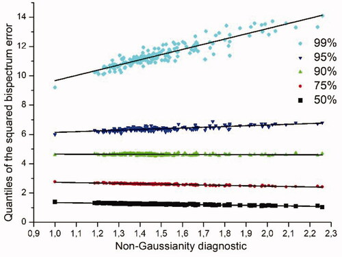
Fig. A3. Position of bifrequencies in the set $L$ used in the integral test of linearity.

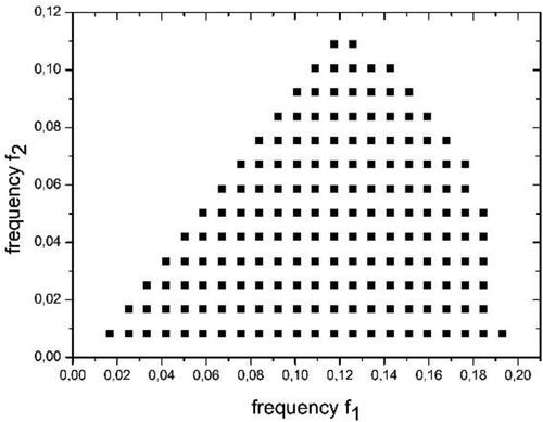
The deviation between the asymptotic variance (A3) and the Monte-Carlo variance $\mathit{var}\left[{\widehat{S}}_{3,\tilde{x}}\right]$(for the real and imaginary parts) is assessed through the ratio: (A5) $${\mathit{var}}_{\mathit{rat}}\left({\widehat{S}}_{3,\tilde{x}}\right)\equiv \frac{\mathit{var}\left({\widehat{S}}_{3,\tilde{x}}\right)}{\frac{M_2^2}{N{b}_2}{\Gamma }_{\tilde{x}}\left(f_1\right){\Gamma }_{\tilde{x}}\left(f_2\right){\Gamma }_{\tilde{x}}\left(f_3\right)},$$(A5) shown in Fig. A1c,d. It can be verified from this figure that when the distance to the principal domain edges or vertices slightly surpasses the bandwidth $\frac{\sqrt{b_2}}{M_2}=0.036 \mathit{cpt},$ then the ratio is nearly constant, varying in the range 0.65–0.80, which is larger than the value 0.5 observed in asymptotic conditions, and hence (A3) underestimates the estimator’s variance (due to sampling ($N_{\mathit{eff}}\ll N$)).

In order to evaluate the distance between the estimated ${\widehat{S}}_{3,x}\left(f_1,f_2\right)$ and the $H_0$ bispectrum, we compute the standardized error (real and imaginary parts): (A6) $$T_{x,\tilde{x}}\left(f_1,f_2\right)\equiv \frac{{\widehat{S}}_{3,x}\left(f_1,f_2\right)-E\left[{\widehat{S}}_{3,\tilde{x}}\right]}{{\left[\mathit{var}\right({\widehat{S}}_{3,\tilde{x}}\left)\right]}^{1/2} }$$(A6)

Asymptotically, under $H_0,$ both real and imaginary parts of $T_{\tilde{x},\tilde{x}}$ are independent standard Gaussian, and ${{ |T}_{\tilde{x},\tilde{x}}|}^2\equiv {Re(T_{x,\tilde{x}})}^2+{Im(T_{x,\tilde{x}})}^2\sim {\chi }_2^2.$ However, for finite samples, $T_{\tilde{x},\tilde{x}}$ tends to be non-Gaussian and leptokurtic and hence the diagnostic ${{\rm Y}}_{\tilde{x}}\equiv \frac{\mathit{var}({{ |T}_{\tilde{x},\tilde{x}}|}^2) }{2E({{ |T}_{\tilde{x},\tilde{x}}|}^2)}$ gets values larger than 1. For the purpose of $H_0$ tests, we also compute the Monte-Carlo quantiles $q_p({{ |T}_{\tilde{x},\tilde{x}}|}^2$). Therefore, the $H_0$ bispectrum is rejected at the frequency pair $\left(f_1,f_2\right)$ if $T_{x,\tilde{x}}\left(f_1,f_2\right)$ or${{ |T}_{x,\tilde{x}}|}^2$ fall outside their $H_0$ nonrejection intervals.

The non-Gaussianity assessment of $T_{\tilde{x},\tilde{x}}$ is presented in Fig. A2, showing ${{\rm Y}}_{\tilde{x}}$ versus $\frac{1}{2}{q}_p\left({{ |T}_{\tilde{x},\tilde{x}}|}^2\right) ,$ for $p=$ 50%, 75%, 90%, 95% and 99%, of the local test ${{ |T}_{\tilde{x},\tilde{x}}|}^2.$ The leftmost points in Fig. A2 are set to the Gaussian case (${{\rm Y}}_{\tilde{x}}=1$) and quantiles are those of ${\frac{1}{2}\chi }_2^2.$ Moreover, quantiles are well adjusted by a linear fitting of ${{\rm Y}}_{\tilde{x}}.$ Quantiles up to $p=$ 95% are well approximated by those of $\frac{1}{2}{\chi }_2^2,$ but less for the whereas the 99%. Consequently, to test $H_0$ by using $T_{x,\tilde{x}}$ and ${{ |T}_{x,\tilde{x}}|}^2,$ with 5% significance or larger, we can use the ${\chi }_2^2.$

The local test (A6) used in Section 5.3.5 is not very powerful because $H_0$ can be rejected at random frequencies even for finite $H_0$ samples. To overcome this an integrated test is used based on the total squared amplitudes: (A7) $$T_{\mathit{int} x,\tilde{x}}\equiv \sum _{\left(f_1,f_2\right)\in L}{{ |T}_{x,\tilde{x}}\left(f_1,f_2\right)|}^2,$$(A7) along $n_L$ bifrequencies of a regularly sampled lattice $L,$ with frequency step, $\Delta f=$ $\frac{5}{N}=0.0084$ cpm, i.e. $\frac{1}{4}$ of the two-dimensional (2D) bandwidth $\frac{\sqrt{b_2}}{M_2}$ to get a good bispectrum representation. ${ T}_{x,\tilde{x}}$ values become uncorrelated when the distance between bifrequencies is typically greater than the 2D bandwidth. The lattice $L$ (Fig. A3) covers the significant region, where $\frac{{\Gamma }_{\tilde{x}}\left(f_1\right){\Gamma }_{\tilde{x}}\left(f_2\right){\Gamma }_{\tilde{x}}\left(f_3\right)}{{{\mathit{Max}}_{PD}(\Gamma }_{\tilde{x}}\left(f_1\right){\Gamma }_{\tilde{x}}\left(f_2\right){\Gamma }_{\tilde{x}}\left(f_3\right)}\ge {\epsilon }_L=0.01$, yielding $n_L=173$ bifrequencies.

Under $H_0,$ the test (A7) has an average $2n_L=346$ and variance equal to 16527, much larger than $\mathit{var}\left({\chi }_{2n_L}^2\right)=692,$ due to correlated bispectrum errors and due to sampled bispectra very far from the theoretical bispectrum. The upper quantiles of $T_{\mathit{int}\tilde{x} ,\tilde{x}}$ for probabilities 80%, 95%, 99% and 99.5% are 489, 563, 804 and 903 respectively, which are the rejection thresholds of NGAR(5) $H_0$ bispectrum, used in Section 5.3.5.

Appendix B:

Minimization of the cost function of the hybrid fitting

B.1. Method

The minimization of $J_{\mathit{hyb}}\left(\mathit{\theta }\right)$ is based on a Quasi–Newton method, and to prevent bad-conditioning, the guess correction is performed along the low-rank subspace spanned by the leading eigenvectors of the Hessian matrix $\mathit{H}:$ (B1) $${\mathit{\theta }}_{k+1}={\mathit{\theta }}_k-\delta {\left[{\mathit{H}}_{lr}\left(J_{\mathit{hyb}}\right({\mathit{\theta }}_k\left)\right)\right]}^{-1}{\mathit{grad}}_{lr}\left(J_{\mathit{hyb}}\right({\mathit{\theta }}_k\left)\right)$$(B1) where $\delta \in ]0,1]$ weights the iteration step, ${\mathit{H}}_{\mathit{lr}}= {\mathit{R}}_{\mathit{lr}}{\mathit{D}}_{\mathit{lr}}{\mathit{R}}_{\mathit{lr}}^{\prime }$ is the low-rank Hessian diagonalisation, and${\mathit{grad}}_{\mathit{lr}}={\mathit{R}}_{\mathit{lr}}\mathit{g}\mathit{rad}$ is the low-rank gradient. The iterative procedure stops when the relative difference between consecutive values is less than 10^–6. The gradient and the Hessian matrix are obtained by time-averages of auxiliary linear models that we describe bellow.

B.2. Gradient of the cost function

The cost function (Eq. (37)) of the hybrid fitting is: (B2) $$J_{\mathit{hyb}}\left(\mathit{\theta }\right)=c_{\mathit{fitt}}{J}_{\mathit{fitt}}\left(\mathit{\theta }\right)+c_{\mathit{stat}}{J}_{\mathit{stat}}\left(\mathit{\theta },{\mathit{\sigma }}_{\mathit{w}}\left(\mathit{\theta }\right)\right)$$(B2) where ${\sigma }_w\mathit{\theta }={\sigma }_x{\left(J_{\mathit{fitt}}\left(\mathit{\theta }\right)\right)}^{1/2}$ and $\mathit{\theta }=({\theta }_1,\dots ,{\theta }_{\mathit{dim}\mathit{\theta }})\mathrm{\prime }.$ The partial derivative of $J_{\mathit{hyb}}$ with respect to ${\theta }_i$ is (B3) $$\frac{\partial J_{\mathit{hyb}}}{\partial {\theta }_i}=c_{\mathit{fitt}}\frac{\partial J_{\mathit{fitt}}}{\partial {\theta }_i}+c_{\mathit{stat}}\left(\frac{\partial J_{\mathit{stat}}}{\partial {\theta }_i}+\frac{\partial J_{\mathit{stat}}}{\partial {\sigma }_w}\frac{\partial {\sigma }_w}{\partial {\theta }_i}\right)$$(B3) where $\frac{\partial {\sigma }_w}{\partial {\theta }_i}=\frac{{\sigma }_w}{2J_{\mathit{fitt}}}\frac{\partial J_{\mathit{fitt}}}{\partial {\theta }_i}.$ The derivatives of $J_{\mathit{fitt}}$ are (B4) $$\frac{\partial J_{\mathit{fitt}}}{\partial {\theta }_i}=\frac{2}{\left(N-N_{\gamma }\right){\sigma }_x^2}\sum _{t=N-N_{\gamma }}^{N-1}\epsilon \left(t\right)\frac{\partial \epsilon \left(t\right)}{\partial {\theta }_i} ,$$(B4) where $ϵ\left(t\right)=x\left(t\right)-F\left[\mathit{x}\left(t-1\right),\mathrm{ }\mathit{\epsilon }\left(t-1\right),\mathrm{ }\mathit{\theta }\right]$ and $\frac{\partial \epsilon (t)}{\partial {\theta }_i}=-\left(\frac{\partial F}{\partial {\theta }_i}+\frac{\partial F}{\partial \mathit{\epsilon }\left(t-1\right)}·\frac{\partial \mathit{\epsilon }\left(t-1\right)}{\partial {\theta }_i}\right)\mathrm{ }$ with the dot standing for inner product along all components of the vector $\mathit{\epsilon }\left(t-1\right)\mathrm{ }$ of past innovations. Those derivatives are random variables governed by an AR linear model whose random coefficients depend on the time-series values. Therefore $\frac{\partial J_{\mathit{fitt}}}{\partial {\theta }_i}$ is approximated by a time average of a product containing the derivative $\frac{\partial \epsilon \left(t\right)}{\partial {\theta }_i}.$

The derivatives of $J_{\mathit{stat}}$ are (B5) $$\begin{array}{c}\frac{\partial J_{\mathit{stat}}}{\partial {\theta }_i}=\frac{2\left({\mathit{S}}_{\mathit{sim}}-{\mathit{S}}_{\mathit{obs}}\right)}{{\mathit{\sigma }}_{\mathit{x}}^2{\mathit{N}}_{\mathit{sim}}}\sum _{t=1}^{N_{\mathit{sim}}}\frac{\partial \tilde{x}\left(t\right)}{\partial {\theta }_i}+\frac{2{\mathit{b}}_1}{{\mathit{\tau }}_{\mathit{max}}{\mathit{\sigma }}_{\mathit{x}}^4 }\sum _{\left|\mathit{\tau }\right|\le {\mathit{\tau }}_{\mathit{max}}}^{}{\mathit{\lambda }\left(\mathit{\tau }\right)}^2\left[{\mathit{C}}_{\mathit{sim}}\left(\mathit{\tau }\right)-{\mathit{C}}_{\mathit{obs}}\left(\mathit{\tau }\right)\right]\frac{\partial {\mathit{C}}_{\mathit{sim}}\left(\mathit{\tau }\right)}{\partial {\mathit{\theta }}_{\mathit{i}}} \\ +\frac{2{\mathit{b}}_2}{{\mathit{\tau }}_{\mathit{max}}^2{\mathit{\sigma }}_{\mathit{x}}^6 }\sum _{\left|{\mathit{\tau }}_1\right|,\left|{\mathit{\tau }}_2\right|\le {\mathit{\tau }}_{\mathit{max}}}^{}{\mathit{\lambda }\left({\mathit{\tau }}_1,{\mathit{\tau }}_2\right)}^2\left[{\mathit{B}}_{\mathit{sim}}\left({\mathit{\tau }}_1,{\mathit{\tau }}_2\right)-{\mathit{B}}_{\mathit{obs}}\left({\mathit{\tau }}_1,{\mathit{\tau }}_2\right)\right]{\frac{\partial {\mathit{B}}_{\mathit{sim}}\left({\mathit{\tau }}_1,{\mathit{\tau }}_2\right)}{\partial {\mathit{\theta }}_{\mathit{i}}} }^{} \end{array}$$(B5) with (B6) $$\frac{\partial C_{\mathit{sim}}\left(\tau \right)}{\partial {\theta }_i}=\frac{1}{N_{\mathit{sim}}-\tau }\sum _{t=1}^{N_{\mathit{sim}}-\tau }\left[\tilde{x}\left(t\right)\frac{\partial \tilde{x}\left(t+\tau \right)}{\partial {\theta }_i}+\tilde{x}\left(t+\tau \right)\frac{\partial \tilde{x}\left(t\right)}{\partial {\theta }_i}\right]$$(B6) (B7) $$\frac{\partial B_{\mathit{sim}}\left({\tau }_1,{\tau }_2\right)}{\partial {\theta }_i}=\frac{1}{N-\mathit{max}({\tau }_1,{\tau }_2)}\sum _{t=1}^{N-\mathit{max}({\tau }_1,{\tau }_2)}\left[\tilde{x}\left(t\right)\tilde{x}\left(t+{\tau }_1\right)\frac{\partial \tilde{x}\left(t+{\tau }_2\right)}{\partial {\theta }_i}+\tilde{x}\left(t\right)\tilde{x}\left(t+{\tau }_2\right)\frac{\partial \tilde{x}\left(t+{\tau }_1\right)}{\partial {\theta }_i}+\tilde{x}\left(t+{\tau }_1\right)\tilde{x}\left(t+{\tau }_2\right)\frac{\partial \tilde{x}\left(t\right)}{\partial {\theta }_i}\right]$$(B7) where $\tilde{x}\left(t\right)=F\left[\tilde{\mathit{x}}\left(t-1\right),\mathrm{ }\mathit{u}\left(t-1\right),\mathrm{ }\mathit{\theta }\right]+{\sigma }_{w}w\left(t\right)$ ,$\mathit{u}\left(t-1\right)={\sigma }_w\mathit{w}\left(t-1\right)$ and $\frac{\partial \tilde{x}\left(t\right)}{\partial {\theta }_i}=\left(\frac{\partial F}{\partial {\theta }_i}+\frac{\partial F}{\partial \tilde{\mathit{x}}\left(t-1\right)}·\frac{\partial \tilde{\mathit{x}}\left(t-1\right)}{\partial {\theta }_i}\right)$ applied to a generic time. An identical formula applies to $\frac{\partial J_{\mathit{stat}}}{\partial {\sigma }_w},$ depending on partial derivatives $\frac{\partial \tilde{x}\left(t\right)}{\partial {\sigma }_w}=\left(\frac{\partial F}{\partial \mathit{u}\left(t-1\right)}·\mathit{w}\left(t-1\right)+\frac{\partial F}{\partial \tilde{\mathit{x}}\left(t-1\right)}·\frac{\partial \tilde{\mathit{x}}\left(t-1\right)}{\partial {\sigma }_w}\right)+w\left(t\right)$ where dot stands for inner products along components of the standard Gaussian past innovations $\mathit{w}\left(t-1\right)$ and components of the past states $\tilde{\mathit{x}}\left(t-1\right).$ Finally, we must see that $\frac{\partial J_{\mathit{stat}}}{\partial {\theta }_i}$ is made by time-averages along the simulation period of a sum of products containing the random derivatives $\frac{\partial \tilde{x}\left(t\right)}{\partial {\theta }_i}.$

The particular form of the derivatives $\frac{\partial u(t)}{\partial {\theta }_i}, \frac{\partial \tilde{x}\left(t\right)}{\partial {\theta }_i},\frac{\partial \tilde{x}\left(t\right)}{\partial {\sigma }_w}$ depend on the stochastic model. In the case of bilinear models (Eq. (29)(29) $$x\left(t,\tau \right)=F\left[\mathit{x}\right(t-1,\tau -1),\mathrm{ }\mathit{ϵ}(t-1,\tau ),\mathrm{ }\mathit{\theta }],$$(29) ), Rao and Gabr (1984) have obtained similar formulas, for $t=0,\dots ,N-1:$ (B8) $$\frac{\partial u\left(t\right)}{\partial a_k}=-\left(x\left(t-l_k\right)+\sum _{i=1}^{p_2}{b}_{i}x\left(t-r_i\right)\frac{\partial u\left(t-s_i\right)}{\partial a_k} \right)$$(B8) (B9) $$\frac{\partial u\left(t\right)}{\partial b_k}=-\left(x\left(t-r_k\right)u\left(t-s_k\right)+\sum _{i=1}^{p_2}{b}_{i}x\left(t-r_i\right)\frac{\partial u\left(t-s_i\right)}{\partial a_k} \right)$$(B9) (B10) $$\frac{\partial u\left(t\right)}{\partial \alpha }=-\left(1+\sum _{i=1}^{p_2}{b}_{i}x\left(t-r_i\right)\frac{\partial u\left(t-s_i\right)}{\partial \alpha } \right),$$(B10) using initial conditions as pseudo-observations $, x\left(t\right)=u\left(t\right)=\frac{\partial u\left(t\right)}{\partial {\theta }_i}=0$ for $, t=-N_{\gamma }-1,\dots ,-1.$ The derivatives of the states are, for $t=0,\dots ,N_{\mathit{sim}}:$ (B11) $$\frac{\partial \tilde{x}\left(t\right)}{\partial a_k}=x\left(t-l_k\right)+\sum _{i=1}^{p_1}{a}_i\frac{\partial \tilde{x}\left(t-l_i\right)}{\partial a_k} +\sum _{i=1}^{p_2}{\sigma }_w{b}_i\frac{\partial \tilde{x}\left(t-r_i\right)}{\partial a_k} w\left(t-s_i\right)$$(B11) (B12) $$\frac{\partial \tilde{x}\left(t\right)}{\partial b_k}={\sigma }_{w}x\left(t-r_k\right)w\left(t-s_k\right)+\sum _{i=1}^{p_1}{a}_i\frac{\partial \tilde{x}\left(t-l_i\right)}{\partial b_k} +\sum _{i=1}^{p_2}{{\sigma }_{w}b}_i\frac{\partial \tilde{x}\left(t-r_i\right)}{\partial b_k} w\left(t-s_i\right)$$(B12) (B13) $$\frac{\partial \tilde{x}\left(t\right)}{\partial \alpha }=1+\sum _{i=1}^{p_1}{a}_i\frac{\partial \tilde{x}\left(t-l_i\right)}{\partial \alpha } +\sum _{i=1}^{p_2}{{\sigma }_{w}b}_i\frac{\partial \tilde{x}\left(t-r_i\right)}{\partial \alpha } w\left(t-s_i\right)$$(B13) (B14) $$\frac{\partial \tilde{x}\left(t\right)}{\partial {\sigma }_w}=w\left(t\right)+\sum _{i=1}^{p_1}{\sigma }_w{a}_i\frac{\partial \tilde{x}\left(t-l_i\right)}{\partial {\sigma }_w} +\sum _{i=1}^{p_2}{{\sigma }_{w}b}_i\frac{\partial \tilde{x}\left(t-r_i\right)}{\partial {\sigma }_w} w\left(t-s_i\right),$$(B14) using initial conditions as pseudo-observations $, \tilde{x}\left(t\right)=\alpha ; w\left(t\right)=\frac{\partial \tilde{x}\left(t\right)}{\partial {\theta }_i}=0 ,\frac{\partial \tilde{x}\left(t\right)}{\partial \alpha }=1$ for $, t=-N_{\mathit{past}},\dots ,0,$ and the derivatives are then substituted into the derivatives of $J_{\mathit{stat}}.$

B.3. Hessian matrix of the cost function

The Hessian matrix is obtained from: (B15) $$\frac{{\partial }^2{J}_{\mathit{hyb}}}{\partial {\theta }_i\partial {\theta }_j}=c_{\mathit{fitt}}\frac{{\partial }^2{J}_{\mathit{fitt}}}{\partial {\theta }_i\partial {\theta }_j}+c_{\mathit{stat}}\left[\frac{{\partial }^2{J}_{\mathit{sta}}}{\partial {\theta }_i\partial {\theta }_j}+\frac{\partial J_{\mathit{stat}}}{\partial {\sigma }_w}\frac{{\partial }^2{\sigma }_w}{\partial {\theta }_j\partial {\theta }_i}+\frac{\partial {\sigma }_w}{\partial {\theta }_i}\frac{{\partial }^2{J}_{\mathit{stat}}}{\partial {\theta }_j\partial {\sigma }_w}+\frac{\partial {\sigma }_w}{\partial {\theta }_j}\frac{{\partial }^2{J}_{\mathit{stat}}}{\partial {\theta }_i\partial {\sigma }_w}+\frac{\partial {\sigma }_w}{\partial {\theta }_i}\frac{\partial {\sigma }_w}{\partial {\theta }_j}\frac{{\partial }^2{J}_{\mathit{stat}}}{\partial {\sigma }_w\partial {\sigma }_w}\right]$$(B15) where $\frac{{\partial }^2{\sigma }_w}{\partial {\theta }_j\partial {\theta }_i}=\frac{{\sigma }_w}{2J_{\mathit{fitt}}}\frac{{\partial }^2{J}_{\mathit{fitt}}}{\partial {\theta }_i\partial {\theta }_j}-\frac{{\sigma }_w}{4J_{\mathit{fitt}}^2}\frac{\partial J_{\mathit{fitt}}}{\partial {\theta }_i}\frac{\partial J_{\mathit{fitt}}}{\partial {\theta }_j}.$ Because the functions involved are sums of squares, we use the approximation of Marquardt (1963), i.e., products of first derivatives. The second derivatives of $J_{\mathit{fitt}}$ are the approximated as (B16) $$\frac{{\partial }^2{J}_{\mathit{fitt}}}{\partial {\theta }_i\partial {\theta }_j}\sim \frac{2}{\left(N-N_{\gamma }\right){\sigma }_x^2}\sum _{t=N-N_{\gamma }}^{N-1}\frac{\partial u\left(t\right)}{\partial {\theta }_i} \frac{\partial u\left(t\right)}{\partial {\theta }_j}$$(B16)

The second derivatives of $J_{\mathit{stat}}$ are then approximated as: (B17) $$\frac{{\partial }^2{J}_{\mathit{stat}}}{\partial {\theta }_i\partial {\theta }_j}\sim \frac{2}{{\sigma }_x^4{N}_{\mathit{sim}}^2}\left[\sum _{t=1}^{N_{\mathit{sim}}}\frac{\partial \tilde{x}\left(t\right)}{\partial {\theta }_i}\right]\left[\sum _{t\prime =1}^{N_{\mathit{sim}}}\frac{\partial \tilde{x}\left(t\prime \right)}{\partial {\theta }_j}\right]+\frac{2b_1}{{\tau }_{\mathit{max}}{\sigma }_x^4 }\sum _{\left|\mathit{\tau }\right|\le {\tau }_{\mathit{max}}}^{}{\lambda \left(\tau \right)}^2\frac{\partial C_{\mathit{sim}}\left(\tau \right)}{\partial {\theta }_i}\frac{\partial C_{\mathit{sim}}\left(\tau \right)}{\partial {\theta }_j} +\frac{2b_2}{{\tau }_{\mathit{max}}^2{\sigma }_x^6 }\sum _{\left|{\tau }_1\right|,\left|{\tau }_2\right|\le {\tau }_{\mathit{max}}}^{}{\lambda \left({\tau }_1,{\tau }_2\right)}^2\frac{\partial B_{\mathit{sim}}\left({\tau }_1,{\tau }_2\right)}{\partial {\theta }_i}{\frac{\partial B_{\mathit{sim}}\left({\tau }_1,{\tau }_2\right)}{\partial {\theta }_j} }^{}$$(B17)

The same formula applies for mixed derivatives with respect to ${\sigma }_w.$

Appendix C:

Symbols and acronyms (by order of appearance)

${ x}_{\mathit{raw}}=$	=	Raw time series
${ x}_{\mathit{cent}}=$	=	Detrended and centered time series
$\sigma \left(x\right)\mathit{\text{ sk}}\left(x\right) \mathit{ekurt}(x)=$	=	Standard deviation, skewness and excess kurtosis of signal $x$
$x(t)=$	=	Standardized time series
$s\left(t\right), f(t)=$	=	Slow and fast components of the standardized time series
$N=$	=	Time series size
$E\left(·\right)=\mathrm{ }$	=	Expectation operator
$N_{\mathit{eff}}=$	=	Number of effective degrees of freedom
$C_x\left(\tau \right)=$	=	Empirical autocovariance
$X_x\left(f\right)\equiv {A_x(f)e}^{[i{\mathrm{\Theta }}_x(f)\mathrm{ }]}=$	=	DFT of the signal $x(t)$ and its polar form
$S_x(f)=$	=	Periodogram
${\Gamma }_x(f)=$	=	Exact spectrum
${\gamma }_x\left(\tau \right)=$	=	Exact autocovariance
${\widehat{S}}_x(f)=$	=	Smoothed spectrum
$\lambda (\tau )=$	=	Window function
$\widehat{\lambda }\left(u\right)=$	=	Standardized window function
$M=$	=	1D window length
$b_1=$	=	Standardized 1D bandwidth
$\nu =$	=	Degrees of freedom of the qui-square
$q_p\left(·\right)=$	=	Quantile por probability p and PDF $\left(·\right)$
$w\left(t\right)=$	=	Zero centered white noise (not necessarily Gaussian nor purely random)
${\sigma }_w=$	=	Standard deviation of the noise
${\sigma }_{w,p}^2=$	=	Noise variance from fitting data with an AR(p) model
${\gamma }_x\left({\tau }_1,{\tau }_2\right)=$	=	Exact bicovariance
$C_x\left({\tau }_1,{\tau }_2\right)=$	=	Empirical bicovariance
$\Delta =$	=	Forecast lag in unit time steps
$x_{nl}(t)=$	=	Nonlinear component of $x(t)$
TCox Δ	=	Cox test for lag $\Delta$ and quantile 95% under the linearity hypothesis
TCox – 95 %	=
$\delta \left(·\right)$	=	Kronecker delta
${\mathrm{\Gamma }}_{3,w}\left(f_1,f_2\right)=$	=	Exact bispectrum
${\Gamma }_{3,y}\left(f_1,f_2\right)=$	=	Normalized exact bispectrum
$S_{3,x}\left(f_1,f_2\right)=$	=	Bi-periodogram
$\mathrm{\Lambda }\left({\tau }_1,{\tau }_2\right)=$	=	2D window function used in the smoothed bispectrum
${\widehat{S}}_{3,x}=$	=	Smoothed bispectrum
${\widehat{S}}_{3n,x}$	=	Smoothed normalized bispectrum
$\delta {\widehat{S}}_{3,x}=$	=	Error of the smoothed bispectrum estimator
${\mathit{var}}_{ar}=$	=	Total smoothed bispectrum error variance under asymptotic conditions
$\overline{(·)}=$	=	Average over the bifrequency domain
${\sigma }_{{\widehat{S}}_{3,x}}=$	=	Typical bispectrum fluctuations
$\tilde{x}(t)=$	=	Null hypothesis model process
$H_0=$	=	Null hypothesis or the null hypothesis model
${\Phi }_{· }=$	=	Standard Gaussian quantile function
$T_{x,\tilde{x}}\left(f_1,f_2\right)=$	=	Standardized bispectrum difference between a model $x$ and $\tilde{x}$
${\mathit{var}}_{\mathit{rat}}({\widehat{S}}_{3,\tilde{x}})=$	=	Ratio between empirical and total asymptotic bispectrum variance
$T_{\mathit{int} x,\tilde{x}}=$	=	Sum of squared amplitudes of $T_{x,\tilde{x}}$ over a certain set $L$ , used to test $H_0$ $\Delta f$
$\Delta f=$	=	Frequency step used in the lattice set $L$
${\epsilon }_L=$	=	Minimum threshold fraction of the asymptotic error variances accepted in $L$
$n_L=$	=	Cardinal of $L$
$A\left(f\right)=$	=	Frequency function intervening in the AR model
$f_{\mathit{cut}}=$	=	Cutoff frequency
${{\rm Y}}_{\tilde{x}}=$	=	Diagnostic of non-Gaussianity of bispectrum errors
$\tilde{x}\left(t\right)=$	=	Simulated state at time $t$
$u\left(t\right)=$	=	Driving noise of a simulating model
$\tilde{\mathit{x}}\left(t-1\right)=$	=	Vector of past simulated states
$\mathit{u}\left(t-1\right)=$	=	Vector of past driving noises or innovations
$J_{\mathit{fitt}}\left(\mathit{\theta }\right) =$	=	Sum of the squared residuals as function of parameters in vector $\mathit{\theta }$
$\epsilon \left(t\right)=$	=	forecasting error at lag 1
$\mathit{\epsilon }\left(t-1\right)=$	=	Vector of past forecasting errors
Npast	=	Size of the trail sector of a simulating time series
$N_{\gamma }=$	=	Maximum lag used in a simulating model
Nsim =	=	Size of the sector of a simulating time series, used to compute statistics
$S_{\mathit{obs}} S_{\mathit{sim}}=$	=	Averages from the observed (obs) and simulated (sim) time series
$C_{\mathit{obs}}\left(\tau \right) C_{sim}\left(\tau \right)=$	=	Noncentered lagged moments of second order for obs. and sim. data
Bobs (T1, T2)	=	Noncentered lagged moments of third order for obs. and sim.
Bsim (T1, T2)	=
$J_S, J_C,J_B=$	=	Normalized squared deviation between the obs. and sim. statistics: average, lagged moments of second and third order respectively
$J_{\mathit{stat}}=$	=	Weighted sum of $J_S, J_C,J_B$ assessing the average deviations between obs. and sim. statistics.
$J_{\mathit{hyb}}=$	=	Weighted sum of $J_{\mathit{fitt}}$ and $J_{\mathit{stat}}$ with weights $c_{\mathit{fitt}}$ and $c_{\mathit{stat}}$ , to minimize in the hybrid fitting
${\mathit{cor}}_{\mathit{lag}}=$	=	Correlation skill between observations and predictions at a certain lag
cpt	=	Cycles per trimester
PD	=	Principal domain, i.e. the triangle of vertices (0,0), (0,1/2) and (1/3,1/3) in the bifrequency domain.
NGAR(5)	=	Non-Gaussian autoregressive model or order 5, used to build the null hypothesis bispectrum
NAIC	=	Normalized Akaike Information Criterion

References

- Ahn, J. H. and Kim, H. S. 2005. Nonlinear modeling of El Nino/southern oscillation index. J. Hydrol. Eng. 10, 8–15. doi:https://doi.org/10.1061/(ASCE)1084-0699(2005)10:1(8)
- Akaike, H. 1974. A new look at the statistical model identification. IEEE Trans. Automat. Contr. 19, 716–723. doi:https://doi.org/10.1109/TAC.1974.1100705
- An, S. I. 2009. A review of interdecadal changes in the nonlinearity of the El Nino-southern oscillation. Theor. Appl. Climatol. 97, 29–40. doi:https://doi.org/10.1007/s00704-008-0071-z
- An, S. I. and Jin, F.-F. 2004. Nonlinearity and asymmetry of ENSO. J. Clim. 17, 2399–2412. doi:https://doi.org/10.1175/1520-0442(2004)017<2399:NAAOE>2.0.CO;2
- An, S. I. and Wang, B. 2000. Interdecadal change of the structure of the ENSO mode and its impact on the ENSO frequency. J. Clim. 13, 2044–2055. doi:https://doi.org/10.1175/1520-0442(2000)013<2044:ICOTSO>2.0.CO;2
- Ashley, R., Patterson, D. and Hinich, M. 1986. A diagnostic test for nonlinear serial dependence in time series fitting errors. J. Time Ser. Anal. 7, 165–178. doi:https://doi.org/10.1111/j.1467-9892.1986.tb00500.x
- Berner, J., Achatz, U., Batté, L., Bengtsson, L., Cámara, A. D. L. and co-authors. 2017. Stochastic parameterization: toward a new view of weather and 574 climate models. Bull. Am. Meteorol. Soc. 98, 565–588. doi:https://doi.org/10.1175/BAMS-D-15-00268.1
- Berner, J., Sardeshmukh, P. D. and Christensen, H. M. 2018. On the dynamical mechanisms governing El Niño-southern oscillation irregularity. J. Clim. 31, 8401–8419. doi:https://doi.org/10.1175/JCLI-D-18-0243.1
- Bianucci, M., Capotondi, A., Mannella, R. and Merlino, S. 2018. Linear or nonlinear modeling for ENSO dynamics? Atmosphere 9, 435. doi:https://doi.org/10.3390/atmos9110435
- Birkelund, Y. and Hanssen, A. 1999. Multitaper estimators for bispectra. Proc. IEEE Workshop on Higher-Order Statistics, Caesarea, Israel, pp. 207–211.
- Birkelund, Y. and Hanssen, A. 2000. Adaptive bispectral estimation using Thomson’s multitaper approach. Proc. IEEE Adaptive Systems for Signal Processing, Communication and Control Symposium, Lake Louise, Alberta, Canada, pp. 283–288.
- Biswas, M., Chandrasekar, A. and Goswami, B. N. 1995. Bispectra of a tropical coupled ocean–atmosphere system. Curr. Sci. 68, 1236–1243. https://www.jstor.org/stable/24096599
- Boucharel, J., Dewitte, B., Garel, B., Penhoat, Y. and Du. 2009. ENSO’s non-stationary and non-Gaussian character: the role of climate shifts. Nonlin. Process. Geophys. 16, 453–473. doi:https://doi.org/10.5194/npg-16-453-2009
- Brillinger, D. 1965. An introduction to polyspectra. Ann. Math. Statist. 36, 1351–1374. doi:https://doi.org/10.1214/aoms/1177699896
- Brillinger, D. and Rosenblatt, M. 1967. Asymptotic theory of k-th order spectra. In: Spectral Analysis of Time Series (ed. B. Harris). John Wiley, New York, pp. 153–188.
- Burgers, G. and Stephenson, D. B. 1999. The ‘normality’ of ENSO. Geophys. Res. Lett. 26, 1027–1030. doi:https://doi.org/10.1029/1999GL900161
- Chunzai, W. 2018. A review of ENSO theories. Natl. Sci. Rev. 5, 813–825. doi:https://doi.org/10.1093/nsr/nwy104.
- Cox, D. R. 1991. Long-range dependence, nonlinearity and time irreversibility. J. Time Ser. Anal. 12, 329–335. doi:https://doi.org/10.1111/j.1467-9892.1991.tb00087.x
- De Gooijer, J. G. 2017. Elements of Nonlinear Time Series Analysis and Forecasting: Springer Series in Statistics. Springer-Verlag, New York. doi:https://doi.org/https://doi.org/10.1007/978-3-319-43252-6.
- Deser, C., Alexander, M. A., Xie, S. P. and Phillips, A. S. 2010. Sea surface temperature variability: patterns and mechanisms. Ann. Rev. Mar. Sci. 2, 115–143.. doi:https://doi.org/10.1146/annurev-marine-120408-151453
- Dijkstra, H. A., Petersik, P., Hernández-García, E. and López, C. 2019. The application of machine learning techniques to improve El Niño prediction skill. Front. Phys. 7, 153. doi:https://doi.org/10.3389/fphy.2019.00153
- Duan, W. and Wei, C. 2013. The ‘spring predictability barrier’ for ENSO predictions and its possible mechanism: results from a fully coupled model. Int. J. Climatol. 33, 1280–1292. doi:https://doi.org/10.1002/joc.3513
- Falguerolles, A. and Francis, B. 1992. Algorithmic approaches for fitting bilinear models. In: Computational Statistics (eds. Y. Dodge and J. Whittaker). Physica, Heidelberg, pp. 77–82. doi:https://doi.org/https://doi.org/10.1007/978-3-662-26811-7_12
- Fan, H., Huang, B., Yang, S., Li, Z. and Deng, K. 2019. Seasonally-dependent impact of easterly wind bursts on the development of El Niño events. Clim. Dyn. 53, 1527–1546. doi:https://doi.org/10.1007/s00382-019-04688-2
- Fedorov, A. V. and Philander, S. G. 2000. Is El Nino changing? Science 288, 1997–2002. doi:https://doi.org/10.1126/science.288.5473.1997
- Franzke, C., Majda, A. J. and Branstator, G. 2007. The origin of nonlinear signatures of planetary wave dynamics: mean phase space tendencies and contributions from non-Gaussianity. J. Atmos. Sci. 64, 3987–4003. doi:https://doi.org/10.1175/2006JAS2221.1
- Frauen, C., Dommenget, D. and Tyrrell, N. 2014. Analysis of the nonlinearity of El Niño-southern oscillation 33721 teleconnections. J. Clim. doi:https://doi.org/10.1175/JCLI-D-13-00757.1
- Gabr, M. M. 1998. Robust estimation of bilinear time series models. Commun. Stat. Theory Methods 27, 41–53. doi:https://doi.org/10.1080/03610929808832649
- Grahn, T. 1995. A conditional least squares approach to bilinear time series estimation. J. Time Ser. Anal. 16, 509–529. doi:https://doi.org/10.1111/j.1467-9892.1995.tb00251.x
- Granger, C. W. J. and Anderson, A. P. 1978. Introduction to Bilinear Time Series Models. Vandenhoeck & Ruprecht, Gottingen.
- Guegan, D. and Pham, D. T. 1989. A note on the estimation of the parameters of the diagonal bilinear model by the method of least squares. Scand. J. Stat. 16, 129–136.
- Haggan, V. and Oyetunji, O. 1980. On the selection of subset autoregressive time series models. UMIST Tech. Report 124. Dept. of Maths, UMIST.
- Hall, A., Skalin, J., & Teräsvirta, T. 2001. A nonlinear time series model of El Niño. Environmental Modelling & Software, 16(2), 139–146. doi: https://doi.org/10.1016/S1364-8152(00)00077–3
- Ham, Y.-G., Kim, J.-H. and Luo, J.-J. 2019. Deep learning for multi-year ENSO forecasts. Nature 573: 568–572. doi:https://doi.org/10.1038/s41586-019-1559-7
- Hannachi, A. and Iqbal, W. 2019. On the nonlinearity of winter northern hemisphere atmospheric variability. J. Atmos. Sci. 76, 333–356. doi:https://doi.org/10.1175/JAS-D-18-0182.1
- Hannachi, A., Straus, D., Franzke, C., Corti, S. and Woollings, T. 2017. Low-frequency nonlinearity and regime behavior in the Northern Hemisphere extratropical atmosphere. Rev. Geophys. 55, 199–234. doi:https://doi.org/10.1002/2015RG000509
- Hinich, J. and Wolinsky, M. A. 1988. A test for aliasing using bispectral analysis source. J. Am. Stat. Assoc. 83, 499–502. doi:https://doi.org/10.1080/01621459.1988.10478623
- Hinich, M. J. 1982. Testing for Gaussianity and linearity of a stationary time series. J. Time Ser. Anal. 3, 169–175. doi:https://doi.org/10.1111/j.1467-9892.1982.tb00339.x
- Hinich, M. J. and Wolinsky, M. A. 2005. Normalizing bispectra. J. Stat. Plann. Inference 130, 405–411. doi:https://doi.org/10.1016/j.jspi.2003.12.022
- Hocke, K. and Kämpfer, N. 2008. Bispectral analysis of the long-term recording of surface pressure at Jakarta. J. Geophys. Res. 113, D10113. doi:https://doi.org/10.1029/2007JD009356
- Jajcay, N., Kravtsov, S., Sugihara, S. G., Tsonis, A. A. and Paluš, M. 2018. Synchronization and causality across time scales in El Niño Southern Oscillation. Clim. Atmos. Sci. 1, 33. doi:https://doi.org/10.1038/s41612-018-0043-7
- Jenkins, G. M. and Watts, D. G. 1968. Spectral Analysis and its Applications. Holden-Day, San Francisco, xviii p. 525.
- Jiang, N., Neelin, J. D. and Ghil, M. 1995. Quasi-quadrennial and quasi-biennial variability in the equatorial Pacific. Clim. Dyn. 12, 101–112. doi:https://doi.org/10.1007/BF00223723
- Kim, Y. C. and Powers, E. J. 1979. Digital Bispectral Analysis and Its Applications to Nonlinear Wave Interactions. IEEE Trans. Plasma Sci. 7, 120–131. doi:https://doi.org/10.1109/TPS.1979.4317207
- Kim, K. Y. 2002. Investigation of ENSO variability using cyclostationary EOFs of observational data. Meteorol. Atmos. Phys. 81, 149–168. doi:https://doi.org/10.1007/s00703-002-0549-7
- Kim, W. K., Billard, L. and Basawa, I. V. 1990. Estimation of the first order diagonal bilinear time series model. J. Time Ser. Anal. 11, 215–230. doi:https://doi.org/10.1111/j.1467-9892.1990.tb00053.x
- Kondrashov, D., Kravtsov, S., Robertson, A. W. and Ghil, M. 2005. A hierarchy of data-based ENSO models. J. Clim. 18, 4425–4444. doi:https://doi.org/10.1175/JCLI3567.1
- Kovach, C. K., Oya, H. and Kawasaki, H. 2018. The bispectrum and its relationship to phase-amplitude coupling. Neuroimage. 173, 518–539. doi:https://doi.org/10.1016/j.neuroimage.2018.02.033
- Kravtsov, S. 2012. An empirical model of decadal ENSO variability. Clim. Dyn. 39, 2377–2391. doi:https://doi.org/10.1007/s00382-012-1424-y
- Lii, K. S. and Rosenblatt, M. 1982. Deconvolution and estimation of transfer function phase and coefficients for non-Gaussian linear processes. Ann. Statist. 10, 1195–1208. doi:https://doi.org/10.1214/aos/1176345984
- Lovejoy, S. 2018. Spectra, intermittency, and extremes of weather, macroweather and climate. Sci. Rep. 8, 1269.
- Marquardt, D. W. 1963. An algorithm for least squares estimation of nonlinear parameters. J. Soc. Indus. Appl. Math. 11, 431–441. doi:https://doi.org/10.1137/0111030
- Martinez-Villalobos, C., Newman, M., Vimont, D. J., Penland, C. and Neelin, J. D. 2019. Observed El Niño-La Niña asymmetry in a linear model. Geophys. Res. Lett. 46, 9909–9919. doi:https://doi.org/10.1029/2019GL082922
- Monahan, A. H. 2020. Bispectral unfolding of the skewness of correlated additive and multiplicative noise processes. Chaos 30, 023126. doi:https://doi.org/10.1063/1.5125787
- Müller, D. 1987. Bispectra of sea-surface temperature anomalies. J. Phys. Oceanogr. 17, 26–36. doi:https://doi.org/10.1175/1520-0485(1987)017<0026:BOSSTA>2.0.CO;2
- Neelin, J. D., Battisti, D. S., Hirst, A. C., Jin, F. F., Wakata, Y. and co-authors. 1998. ENSO theory. J. Geophys. Res. 103, 14261–14290. doi:https://doi.org/10.1029/97JC03424
- Nikias, C. L. and Raghuveer, M. R. 1987. Bispectrum estimation: a digital signal processing framework. Proc. IEEE 75, 869–891. doi:https://doi.org/10.1109/PROC.1987.13824
- Penland, C. 1996. A stochastic model of Indo-Pacific sea-surface temperature anomalies. Phys. D 98, 534–558. doi:https://doi.org/10.1016/0167-2789(96)00124-8
- Pham, D. T. and Tran, L. T. 1981. On the first order bilinear time series models. J. Appl. Prob. 18, 617–627. doi:https://doi.org/10.2307/3213316
- Pires, C. and Hannachi, A. 2017. Independent subspace analysis of the sea surface temperature variability: non-Gaussian sources and sensitivity to sampling and dimensionality. Complexity 2017, 1–23. doi:https://doi.org/10.1155/2017/3076810
- Pires, C. and Perdigão, R. 2015. Non-Gaussian interaction information: estimation, optimization and diagnostic application of triadic wave resonance. Nonlin. Process. Geophys. 22, 87–108. doi:https://doi.org/10.5194/npg-22-87-2015
- Pires, C. A., Talagrand, O. and Bocquet, M. 2010. Diagnosis and impacts of non-Gaussianity of innovations in data assimilation. Phys. D 239, 1701–1717. doi:https://doi.org/10.1016/j.physd.2010.05.006
- Priestley, M. B. 1981. Spectral Analysis and Time Series 1. Academic, New York.
- Privalsky, V. and Muzylev, S. 2013. An experimental stochastic model of the El Niño-Southern oscillation system at climatic time scales. Univ. J. Geosci. 1, 28–36. http://www.hrpub.org.
- Proistosescu, C., Rhines, A. and Huybers, P. 2016. Identification and interpretation of nonnormality in atmospheric time series. Geophys. Res. Lett. 43, 5425–5434. doi:https://doi.org/10.1002/2016GL068880
- Raghuveer, M. R. and Nikias, C. L. 1986. Bispectrum estimation via AR modeling. Signal Process. 10, 35–48. doi:https://doi.org/10.1016/0165-1684(86)90063-0
- Rao, S. S., Rao, T. S. and Rao, C. R. 2012. Time Series Analysis: Methods and Applications, Vol. 30, Elsevier Science and Technology, North-Holland.
- Rao, T. S. 1981. On the theory of bilinear time series models. J. R. Statist. Soc. B 43, 2, 244–255.
- Rao, T. S. and Gabr, M. M. 1984. Bilinear time series models. In: An Introduction to Bispectral Analysis and Bilinear Time Series Models. Lecture Notes in Statistics, Vol. 24, Springer, New York, NY.
- Rayner, N. A., Parker, D. E., Horton, E. B., Folland, C. K., Alexander, L. V. and co-authors. 2003. Global analyses of sea surface temperature, sea ice, and night marine air temperature since the late nineteenth century. J. Geophys. Res. 108, 4407. 2003. doi:https://doi.org/10.1029/2002JD002670
- Richardson, A. M. and Hodgkiss, W. S. 1994. Bispectral analysis of underwater acoustic data. J. Acoust. Soc. Am. 96, 828–837. doi:https://doi.org/10.1121/1.410321
- Rusticelli, E., Ashley, R. A., Dagum, E. B. and Patterson, D. M. 2008. A new bispectral test for nonlinear serial dependence. Econ. Rev. 28, 279–293. doi:https://doi.org/10.1080/07474930802388090
- Sardeshmukh, P. D. and Sura, P. 2009. Reconciling non-Gaussian climate statistics with linear dynamics. J. Clim. 22, 1193–1207. doi:https://doi.org/10.1175/2008JCLI2358.1
- Schulte, J., Policielli, F. and Zaitchik, B. 2020. A skewed perspective of the Indian rainfall–ENSO relationship. Hydrol. Earth Syst. Sci., 24, 5473–5489. doi:https://doi.org/10.5194/hess-24-5473-2020
- Sesay, S. A. O. and Rao, T. S. 1988. Yule–Walker type difference equations for higher-order moments and cumulants for bilinear time series models. J. Time Ser. Anal. 9, 385–401. doi:https://doi.org/10.1111/j.1467-9892.1988.tb00478.x
- Stein, K., Timmermann, A., Schneider, N., Jin, F.-F. and Stuecker, M. F. 2014. ENSO seasonal synchronization theory. J. Clim. 27, 5285–5310. doi:https://doi.org/10.1175/JCLI-D-13-00525.1
- Stuecker, M. F., Timmermann, A., Jin, F.-F., McGregor, S. and Ren, H.-L. 2013. A combination mode of the annual cycle and the El Niño/Southern oscillation. Nat. Geosci. 6, 540–544. doi:https://doi.org/10.1038/ngeo1826
- Sun, F. and Yu, J.-Y. 2009. A 10–15-yr modulation cycle of ENSO intensity. J. Clim. 22, 1718–1735. doi:https://doi.org/10.1175/2008JCLI2285.1
- Sura, P. and Hannachi, A. 2015. Perspectives of non-Gaussianity in atmospheric synoptic and low-frequency variability. J. Clim. 28, 5091–5114. doi:https://doi.org/10.1175/JCLI-D-14-00572.1
- Sura, P. and Sardeshmukh, P. 2008. A global view of non-Gaussian SST variability. J. Phys. Oceanogr. 38, 639–647. doi:https://doi.org/10.1175/2007JPO3761.1
- Takens, F., Rand, D. A. and Young, D. S., eds. 1981. Dynamical Systems and Turbulence (Warwick 1980), Lecture Notes in Mathematics, Vol. 898, Springer, Berlin, 365 pp.
- Tang, Y., Zhang, R. H., Liu, T., Duan, W., Yang, D. and co-authors. 2018. Progress in ENSO prediction and predictability study. Natl. Sci. Rev. 5, 826–839. doi:https://doi.org/10.1093/nsr/nwy105
- Tang, Z. and Mohler, R. R. 1988. Bilinear time series: theory and applications. In Lecture Notes in Control and Information Sciences (eds. M. Thoma and A. Wyner), 106, pp. 43–58. Springer-Verlag, Berlin.
- Timmermann, A. 2003. Decadal ENSO amplitude modulations: a nonlinear paradigm. Glob Planet Change 37, 135–156. doi:https://doi.org/10.1016/S0921-8181(02)00194-7
- Timmermann, A., An, S.-I., Kug, J.-S., Jin, F.-F., Cai, W. and co-authors. 2018. El Niño-Southern oscillation complexity. Nature 559, 535–545. doi:https://doi.org/https://doi.org/10.1038/s4158 6-018-0252-6
- Timmermann, A., Voss, H. U. and Pasmanter, R. 2001. Empirical dynamical system modeling of ENSO using nonlinear inverse techniques. J. Phys. Oceanogr. 31, 1579–1598. doi:https://doi.org/10.1175/1520-0485(2001)031<1579:EDSMOE>2.0.CO;2
- Ubilava, D. and Helmers, C. G. 2013. Forecasting ENSO with a smooth transition autoregressive model. Environ. Model. Softw. 40, 181–190. doi:https://doi.org/10.1016/j.envsoft.2012.09.008
- Usoro, A. E. 2015. Comparative analysis of linear and bilinear time series models American. J. Math. Stat. 5, 265–271.
- von Storch, H. and Zwiers, F. W. 1999. Statistical Analysis in Climate Research. Cambridge University Press, Cambridge, 484 p. doi: https://doi.org/10.1017/CBO9780511612336
- Wang, C. 2018. A review of ENSO theories. Natl. Sci. Rev. 5, 813–825. doi:https://doi.org/10.1093/nsr/nwy104
- Wang, C., Deser, C., Yu, J.-Y., DiNezio, P., and Clement, A. 2016. El Niño-Southern Oscillation (ENSO): a review. In Coral Reefs of the Eastern Pacific (eds. P. Glymn, D. Manzello, and I. Enochs). Springer Science Publisher, Berlin, pp. 85–106.
- Weiss, G. 1975. Time-reversibility of linear stochastic processes. J. Appl. Prob. 12, 831–836. doi:https://doi.org/10.2307/3212735
- Wilks, D. S. 2011. Statistical Methods in the Atmospheric Sciences. 3rd ed. Elsevier, Academic Press, Amsterdam.
- Woollings, T., Hannachi, A. and Hoskins, B. 2010. Variability of the North Atlantic eddy-driven jet stream. QJR. Meteorol. Soc. 136, 856–868. doi:https://doi.org/10.1002/qj.625
- Wu, A. and Hsieh, W. W. 2003. Nonlinear interdecadal changes of the El Niño-Southern oscillation. Clim. Dyn. 21, 719–730. doi:https://doi.org/10.1007/s00382-003-0361-1
- Yeh, S.-W. and Kirtman, B. P. 2004. Tropical Pacific decadal variability and ENSO amplitude modulation in a CGCM. J. Geophys. Res. 109, C11009. doi:https://doi.org/10.1029/2004JC002442
- Yishuai, J., Zhengyao, L. and Zhengyu, L. 2020. Controls of spring persistence barrier strength in different ENSO regimes and implications for 21st century changes. Geophys. Res. Lett. 47, 11. https://doi.org/10.1029/2020GL088010.
- Zhang, Y., Wallace, J. M. and Battisti, D. S. 1997. ENSO‐like interdecadal variability: 1900–93. J. Clim. 10, 1004–1020. doi:https://doi.org/10.1175/1520-0442(1997)010<1004:ELIV>2.0.CO;2