Energetics characteristics accounting for the low-level wind’s rapid enhancement associated with an extreme explosive extratropical cyclone over the western North Pacific Ocean

ABSTRACT

During mid-January 2011, a rarely seen twin-extratropical-cyclone event appeared over the western North Pacific Ocean. One of the twin cyclones developed into an extreme explosive extratropical cyclone (EEC), which was comparable to the intensity of a typhoon. Rotational and divergent wind kinetic energy (KE) analyses were applied to understand the low-level wind’s rapid enhancement associated with the cyclone. It was found that: (i) the total wind KE associated with the EEC showed a remarkable enhancement in the lower troposphere during the cyclone’s maximum development stage, with the maximum/minimum wind acceleration appearing in the southeastern/northwestern quadrant of the EEC; (ii) the rotational wind KE experienced an obvious increase, which corresponded to the total wind KE enhancement, whereas the divergent wind KE, which was much smaller than the rotational wind, mainly featured a decreasing trend; (iii) the rotational wind KE enhancement showed variational features consistent with the horizontal enlargement and upward stretching of the EEC; (iv) the nonorthogonal wind KE enhanced the total wind KE in regions with strong rotational wind, which resulted in the maximum lower-tropospheric maximum wind, whereas in regions with strong divergent wind it mainly reduced the total wind KE; (v) the northward transport of total wind KE and the rotational wind KE production due to the work done by pressure gradient force were dominant factors for the enhancement of winds associated with the EEC, particularly in its southeastern section. In contrast, an overall conversion from rotational wind KE to divergent wind KE decelerated the rotational wind enhancement.

Graphical abstract

摘要

2011年一月中旬, 西北太平洋上发生了一次罕见的双子气旋事件。该双子气旋中的一个气旋 (简称气旋A) 迅速发展成为一个强度堪比台风的极端强度爆发气旋。本文采用旋转风, 辐散风动能收支分析来研究造成该极端强度爆发气旋风速迅速增强的原因。研究发现, 在气旋A的最快发展期, 对流层低层, 气旋的总动能迅速增大, 风速增大最迅速的象限是气旋的东南象限, 而西北象限的增速最慢。旋转风动能的增长显著, 对应了总动能的增大, 而辐散风的动能显著小于旋转风动能并且主要表现出减少的趋势。旋转风动能的增大与气旋A在水平和垂直方向上的伸展过程相一致, 非正交风动能在旋转风动能大值区增强总动能, 这促使了对流层低层最大风速的形成, 然而, 在辐散风动能较强的区域, 非正交风动能主要减弱总动能。向北的总动能输送以及气压梯度力对旋转风动能的做功是气旋A风速迅速增大的主导因子, 尤其是在其东南象限。然而, 从旋转风向辐散风动能的转换在一定程度上延缓了气旋风速的增强过程。

KEYWORDS:

• Explosive extratropical cyclone
• rotational wind
• divergent wind
• kinetic energy
• twin cyclones

关键词:

• 爆发气旋
• 旋转风
• 辐散风
• 动能
• 双子气旋

1. Introduction

Explosive extratropical cyclones (EECs), which have a deepening rate of at least 1 Bergeron (i.e., a geostrophically equivalent deepening rate of 24 hPa/24 h), are an important subcategory of extratropical cyclones (Sanders and Gyakum 1980; Yoshida and Asuma 2004). During the rapid deepening process of an EEC, snowstorms, strong winds, severe cold waves, and massive waves are often observed (Qi 1993; Fu, Sun, and Sun 2014), which pose serious threats to not only the fishery and shipping industries but also to the coastal areas in middle to high latitudes.

Because of their enormous destructive power, EECs have been a research hotspot for many decades (Schultz et al. 2019). For instance, Sanders and Gyakum (1980) applied a four-year statistical analysis to EECs and found that their rapid enhancement was closely correlated with the strongest gradients of sea surface temperature. Chen and Dell’osso (1987) found sensible heating could accelerate EECs’ rapid deepening. Using the Zwack–Okossi equations (Zwack and Okossi 1986), Lupo, Smith, and Zwack (1992) proposed that cyclonic-vorticity advection, warm advection, and condensation induced the rapid cyclogenesis, whereas adiabatic cooling in ascending air decelerated the development. Hakim, Keyser, and Bosart (1996) analyzed an EEC during a wave merging and found a preexisting upper-level disturbance dominated the explosive cyclogenesis. Yoshida and Asuma (2004) focused on EECs over the western North Pacific region. Through composite analyses, they proposed that the presence and extension of a cold air mass over the Asian continent were favorable to the explosive development. Kuwano-Yoshida and Asuma (2008) conducted sensitivity experiments on three extreme EECs over the Northwest Pacific Ocean. They proposed that latent heating affected the rapid deepening mainly through nonlinear interactions with an upper-level jet and shortwave trough. Wu, Martin, and Petty (2011) and Fu, Sun, and Sun (2014) applied piecewise potential vorticity inversion analyses to EECs over the Northwest Pacific Ocean. Their results confirmed the significance of the upper-level perturbations and latent heating in causing explosive cyclogeneses.

During mid-January 2011, an extreme EEC appeared over the western North Pacific Ocean, which had comparable intensity to that of a typhoon. Results from Fu et al. (2018) indicated that strong warm advection in the upper troposphere, positive potential-vorticity (induced by tropopause folding), and latent heating (due to condensation) in the middle troposphere, as well as warm advection in the lower troposphere, were favorable conditions for the rapid development of this cyclone. However, which governed the EEC-related strong low-level wind’s (which caused extremely strong cold waves and massive waves) formation, is still unknown. As a continuation to the study of Fu et al. (2018), the present work attempts to understand the low-level wind’s rapid enhancement associated with the EEC by conducting kinetic energy (KE) analysis and budget calculation. The remainder of this paper is structured as follows: the data and methods used in this study are described in Section 2; the main results are reported in Section 3; and a conclusion is presented in Section 4.

2. Data and methods

2.1. Data

This study conducted analyses based on the simulation results from Fu et al. (2018), who reproduced the extreme EEC event over the western North Pacific Ocean in mid-January 2011 reasonably well (Section 3.1 in Fu et al. (2018)). The simulation used the fifth-generation Pennsylvania State University Mesoscale Model, version 3.7 (Grell, Dudhia, and Stauffer 1995). Two one-way nested domains (36 km and 12 km) were utilized in the simulation. Six-hourly National Centers for Environmental Prediction final analysis data with a resolution of 1° × 1° were used for the initial and boundary conditions of the simulation. Weekly mean optimum interpolated sea surface temperature data (1° × 1°) from the Climate Diagnostics Center of the National Oceanic and Atmospheric Administration’s Cooperative Institute for Research in Environmental Sciences (Reynolds et al. 2002) were used as sea surface temperature conditions. Surface, rawinsonde, ship, and buoy observations from the Japan Meteorological Agency were employed to improve the initial conditions of the simulation in the outer domain. The model was integrated for 192 h to cover the EEC’s entire lifetime. A simple-ice explicit moisture scheme (Dudhia 1989) was used in the outer domain, a mixed-phase scheme (Reisner, Rasmussen, and Bruintjes 1998) was employed in the inner domain, and the Grell cumulus scheme (Grell 1993) was used in both domains. All analyses and calculations in this study were based on the hourly output from the inner domain. More detailed information about the simulation and its validation are documented in Fu et al. (2018).

2.2. Methods

The Helmholtz theorem indicates that the horizontal wind can be decomposed into the rotational wind and divergent wind (Hawkins and Rosenthal 1965; Lynch 1988). Previous studies have shown rotational and divergent wind KE can represent the variation of a cyclone effectively (Ding and Liu 1985; Buechler and Fuelberg 1986; Fu et al. 2011, 2012). Therefore, this study employed the rotational and divergent wind KE analyses and budgets to understand the wind variation of the extreme EEC. The equations from Buechler and Fuelberg (1986) shown as follows were used in this study:

(1) $\begin{array}{rl}& \frac{\mathrm{\partial }{k}_{\mathrm{R}}}{\mathrm{\partial }t}=-V_{\mathrm{R}}\cdot \frac{\mathrm{\partial }{V}_{\mathrm{D}}}{\mathrm{\partial }t}+C\left(k_{\mathrm{D}},k_{\mathrm{R}}\right)-V_{\mathrm{R}}\cdot \mathrm{\nabla }\mathrm{\Phi }-\mathrm{\nabla }\cdot \left(V_{\mathrm{R}}k\right)+V_{\mathrm{R}}\cdot F,\\ & \mathrm{R}1\mathrm{C}\mathrm{O}\mathrm{N}\mathrm{R}2\mathrm{R}3\mathrm{R}4\end{array}$(1)

(2) $\begin{array}{rl}& \frac{\mathrm{\partial }{k}_{\mathrm{D}}}{\mathrm{\partial }t}=-V_{\mathrm{D}}\cdot \frac{\mathrm{\partial }{V}_{\mathrm{R}}}{\mathrm{\partial }t}-C\left(k_{\mathrm{D}},k_{\mathrm{R}}\right)-V_{\mathrm{D}}\cdot \mathrm{\nabla }\mathrm{\Phi }\\ & \mathrm{D}1\mathrm{C}\mathrm{O}\mathrm{N}\mathrm{D}2\\ & -\mathrm{\nabla }\cdot \left(V_{\mathrm{D}}k\right)-\frac{\mathrm{\partial }\left(\omega k\right)}{\mathrm{\partial }p}+V_{\mathrm{D}}\cdot F,\\ & \mathrm{D}3\mathrm{D}4\mathrm{D}5\end{array}$(2)

(3) $C\left(k_{\mathrm{D}},k_{\mathrm{R}}\right)=-\left(\zeta +f\right)\left(-u_{\mathrm{R}}{v}_{\mathrm{D}}+v_{\mathrm{R}}{u}_{\mathrm{D}}\right)-\omega \frac{\mathrm{\partial }{k}_{\mathrm{R}}}{\mathrm{\partial }p}-\omega \left(u_{\mathrm{R}}\frac{\mathrm{\partial }{u}_{\mathrm{D}}}{\mathrm{\partial }p}+v_{\mathrm{R}}\frac{\mathrm{\partial }{v}_{\mathrm{D}}}{\mathrm{\partial }p}\right),$(3)

where ${\mathit{V}}_{\mathrm{R}}=u_{\mathrm{R}}\mathit{i}+v_{\mathrm{R}}\mathit{j}$ is the rotational wind vector; ${\mathit{V}}_{\mathrm{D}}=u_{\mathrm{D}}\mathit{i}+v_{\mathrm{D}}\mathit{j}$ is the divergent wind vector; ${\mathit{V}}_h={\mathit{V}}_{\mathrm{R}}+{\mathit{V}}_{\mathrm{D}}$ is the total wind vector; and $k_{\mathrm{R}}=\frac{1}{2}{\mathit{V}}_{\mathrm{R}}\cdot {\mathit{V}}_{\mathrm{R}}$, $k_{\mathrm{D}}=\frac{1}{2}{\mathit{V}}_{\mathrm{D}}\cdot {\mathit{V}}_{\mathrm{D}}$, $k=\frac{1}{2}{\mathit{V}}_h\cdot {\mathit{V}}_h$ are the rotational, divergent, and total wind KE, respectively. They satisfy a relationship $k=k_{\mathrm{R}}+k_{\mathrm{D}}+{\mathit{V}}_{\mathrm{R}}\cdot {\mathit{V}}_{\mathrm{D}}$, where ${\mathit{V}}_{\mathrm{R}}\cdot {\mathit{V}}_{\mathrm{D}}$ is defined as the nonorthogonal wind KE. $\mathrm{\nabla }$ is the three-dimensional gradient operator, $\mathrm{\Phi }$ is the geopotential, $\mathit{F}$ is the frictional force, p is pressure, f is the Coriolis parameter, ζ is relative vorticity, and ω is vertical velocity in the pressure coordinate.

Rotational and divergent wind in this study were calculated by using the method developed by Xu, Cao, and Gao (2011), which has been proven to be effective and accurate. In Equation (1)(1) $\begin{array}{rl}& \frac{\mathrm{\partial }{k}_{\mathrm{R}}}{\mathrm{\partial }t}=-V_{\mathrm{R}}\cdot \frac{\mathrm{\partial }{V}_{\mathrm{D}}}{\mathrm{\partial }t}+C\left(k_{\mathrm{D}},k_{\mathrm{R}}\right)-V_{\mathrm{R}}\cdot \mathrm{\nabla }\mathrm{\Phi }-\mathrm{\nabla }\cdot \left(V_{\mathrm{R}}k\right)+V_{\mathrm{R}}\cdot F,\\ & \mathrm{R}1\mathrm{C}\mathrm{O}\mathrm{N}\mathrm{R}2\mathrm{R}3\mathrm{R}4\end{array}$(1) , term R1 represents the work done by divergent wind, R2 denotes the work done by pressure gradient force, R3 reflects the transport of k by rotational wind, and R4 stands for frictional-force’s work. In Equation (2)(2) $\begin{array}{rl}& \frac{\mathrm{\partial }{k}_{\mathrm{D}}}{\mathrm{\partial }t}=-V_{\mathrm{D}}\cdot \frac{\mathrm{\partial }{V}_{\mathrm{R}}}{\mathrm{\partial }t}-C\left(k_{\mathrm{D}},k_{\mathrm{R}}\right)-V_{\mathrm{D}}\cdot \mathrm{\nabla }\mathrm{\Phi }\\ & \mathrm{D}1\mathrm{C}\mathrm{O}\mathrm{N}\mathrm{D}2\\ & -\mathrm{\nabla }\cdot \left(V_{\mathrm{D}}k\right)-\frac{\mathrm{\partial }\left(\omega k\right)}{\mathrm{\partial }p}+V_{\mathrm{D}}\cdot F,\\ & \mathrm{D}3\mathrm{D}4\mathrm{D}5\end{array}$(2) , term D1 represents the work done by rotational wind, D2 denotes the work done by pressure gradient force, D3 reflects the transport of k by divergent wind, D4 is the vertical transport of k, and D5 stands for frictional-force’s work. Term CON denotes the conversion between the rotational and divergent wind KE, which has three components as Equation (3)(3) $C\left(k_{\mathrm{D}},k_{\mathrm{R}}\right)=-\left(\zeta +f\right)\left(-u_{\mathrm{R}}{v}_{\mathrm{D}}+v_{\mathrm{R}}{u}_{\mathrm{D}}\right)-\omega \frac{\mathrm{\partial }{k}_{\mathrm{R}}}{\mathrm{\partial }p}-\omega \left(u_{\mathrm{R}}\frac{\mathrm{\partial }{u}_{\mathrm{D}}}{\mathrm{\partial }p}+v_{\mathrm{R}}\frac{\mathrm{\partial }{v}_{\mathrm{D}}}{\mathrm{\partial }p}\right),$(3) shows. Two total (TOT) terms are defined as TOT_R = R1 + R2 + R3 + CON and TOT_D = D1 + D2 + D3 + D4 − CON, respectively, which show the total effect of the right-hand side terms except for the friction-related effects.

3. Results

3.1. Overview of the event

At 1500 UTC 15 January, a twin-extratropical-cyclones event appeared over the western North Pacific Ocean (Figure 1 in Fu et al. (2018)). The twin cyclones showed a significant Fujiwhara effect, during which they orbited cyclonically about a midpoint, drew closer to each other with time, and finally, the initial stronger cyclone (named Cyclone B) merged into the initial weaker cyclone (named Cyclone A). Cyclone A featured a deepening rate of up to 2.6 Bergeron (Figure 2 of Fu et al. (2018)) from 0000 UTC 16 to 0000 UTC 17 January (it was defined as the maximum development stage), which means it was an extreme EEC according to the standard documented in Yoshida and Asuma (2004). Around 0000 UTC 17 January, a maximum surface wind of ~33 m s⁻¹ appeared in the southeastern section of the cyclone, and by 1800 UTC 17 January a minimum sea level pressure of ~933 hPa appeared in the cyclone center, implying Cyclone A was comparable with the intensity of a typhoon (Ying et al. 2014). After that, Cyclone A began to fill and dissipated at 1200 UTC 22 January (this cyclone lasted for a total of ~165 h). Because the maximum development stage showed the most rapid deepening rate and largest lower-tropospheric wind, this study mainly focused on this stage to answer the scientific question raised in the introduction.

Figure 1. The left-hand column shows the 900-hPa total wind KE (shading; units: J kg⁻¹) and nonorthogonal wind KE (black lines with an interval of 20 J kg⁻¹). The right-hand column shows the 900-hPa rotational wind KE (shading; units: J kg⁻¹) and divergent wind KE (black lines with an interval of 10 J kg⁻¹). The red solid box shows the central region (12° × 12°) of Cyclone A, and the purple dashed boxes illustrate 16 key regions (6° × 6°) of the cyclone.

Figure 2. Total region (a) and each key region (b–q) averaged rotational (shading; units: J kg⁻¹) and divergent wind KE (black solid lines with an interval of 2 J kg⁻¹), where the solid purple line marks the top level of the cyclone and the gray-dashed lines show the maximum development stage.

3.2. Energetics features

As documented in Fu et al. (2018), 900 hPa was used as the representative level of Cyclone A, and the red box shown in Figure 1(a) (12° × 12°) was used as the central region of the cyclone. Because the wind maximum associated with the cyclone was outside the central region (Figure 1), we defined a double side-length box, which centered in the centroid of Cyclone A, as the largest purple dashed box in Figure 1(a) (24° × 24°) shows. Correspondingly, 16 key regions were defined to investigate the main features of the cyclone, as the small purple and red boxes (6° × 6°) in Figure 1(a) illustrate.

From Section 2.2, the total wind KE could be decomposed into the rotational wind KE, divergent wind KE, and nonorthogonal wind KE, which are shown in Figure 1. It can be seen that the total wind KE associated with the cyclone grew with time, implying enhancement in wind of the cyclone. Overall, the southeastern section of the cyclone showed larger total wind KE than other sections (Figure 1(a–d)), with strong 900-hPa wind maxima above 40 m s⁻¹ appearing in the key region IV4 around 0000 UTC 17 January. Although the rotational wind KE was generally smaller than the total wind KE, it showed the most similar distribution, intensity, and evolution to those of the total wind KE (Figure 1(e–h)). This means the rotational wind KE was the dominant component of the total wind. The rotational wind KE and divergent wind KE showed remarkably different features: (i) the former was one to two orders of magnitude larger than the latter (Figure 1(e–h)); (ii) key regions I1 and I4, which featured strong low-level convergence (not shown), generally showed divergent wind KE maxima, whereas rotational wind KE maxima were mainly located in key regions IV1–4; and (iii) the intensity of the rotational wind KE was mainly increasing with time, while that of the divergent wind KE was mainly decreasing.

The nonorthogonal wind KE, which acted as a link among the total wind KE as well as the rotational and divergent wind KE, could have negative values. This is because its sign is determined by the angle between the rotational and divergent wind. If the angle is less than 90°, it is positive, which amplifies the total wind KE; whereas, if the angle is larger than 90°, it reduces the total wind. Comparing the maxima of total wind KE (key regions IV1–4) with those of rotational wind KE (c.f., Figure 1(a–h)), it can be seen that the nonorthogonal wind KE mainly enhanced the total wind KE in those regions with strong rotational wind KE, which enhanced the total wind KE. In contrast, in the regions featuring strong divergent wind KE (e.g., key regions II1, I1, and I4), overall, negative nonorthogonal wind KE was also large, which mainly reduced the total wind KE there.

Figure 2 shows the key-region-averaged rotational and divergent wind KE, from which it can be seen that: (i) rotational wind KE was one to two orders of magnitude larger than divergent wind KE; (ii) rotational wind KE maximized in the upper troposphere and decreased downward; and (iii) divergent wind KE also maximized in the upper troposphere but minimized in the middle troposphere (which was consistent with the vertical distribution of divergence). During the maximum development stage, overall, Cyclone A showed a remarkable enhancement in lower-tropospheric (below 700 hPa) rotational wind KE and a rapid upward extension (thick purple solid line in Figure 2(a)), both of which corresponded to the explosive development of the cyclone. In contrast, the middle-(400–700 hPa) and upper-tropospheric (above 400 hPa) rotational wind KE featured a slow variation and an obvious reduction, respectively.

The 16 key regions of Cyclone A showed significantly different KE features (Figure 2(b–q)). Overall, in the upper troposphere, rotational wind KE was much stronger in the southern section of the cyclone (e.g., key regions III1–4 and IV1–4) than that in the northern section (e.g., key regions I1–4 and II1–4), because an upper-level jet core was located over the southern section (Fu et al. 2018). Among all 16 key regions, except for key regions III2–3, IV1, IV2, and IV4, all other key regions mainly featured a decrease in upper-tropospheric rotational wind KE during the maximum development stage. Moreover, except for key regions II3–4 and III2–4, the other 11 key regions all showed an enhancement in the low-level rotational wind KE in the same stage (Figure 2(b–q)). Overall, key regions IV1–4 featured the largest lower-tropospheric rotational wind KE (maximum surface wind velocity appeared in key region IV4) and most rapid rotational wind enhancement, and therefore they were selected as representative for understanding how the strong winds associated with the EEC formed.

3.3. KE budget results

Before analyzing the budget results from Equations (1)(1) $\begin{array}{rl}& \frac{\mathrm{\partial }{k}_{\mathrm{R}}}{\mathrm{\partial }t}=-V_{\mathrm{R}}\cdot \frac{\mathrm{\partial }{V}_{\mathrm{D}}}{\mathrm{\partial }t}+C\left(k_{\mathrm{D}},k_{\mathrm{R}}\right)-V_{\mathrm{R}}\cdot \mathrm{\nabla }\mathrm{\Phi }-\mathrm{\nabla }\cdot \left(V_{\mathrm{R}}k\right)+V_{\mathrm{R}}\cdot F,\\ & \mathrm{R}1\mathrm{C}\mathrm{O}\mathrm{N}\mathrm{R}2\mathrm{R}3\mathrm{R}4\end{array}$(1) and (2(2) $\begin{array}{rl}& \frac{\mathrm{\partial }{k}_{\mathrm{D}}}{\mathrm{\partial }t}=-V_{\mathrm{D}}\cdot \frac{\mathrm{\partial }{V}_{\mathrm{R}}}{\mathrm{\partial }t}-C\left(k_{\mathrm{D}},k_{\mathrm{R}}\right)-V_{\mathrm{D}}\cdot \mathrm{\nabla }\mathrm{\Phi }\\ & \mathrm{D}1\mathrm{C}\mathrm{O}\mathrm{N}\mathrm{D}2\\ & -\mathrm{\nabla }\cdot \left(V_{\mathrm{D}}k\right)-\frac{\mathrm{\partial }\left(\omega k\right)}{\mathrm{\partial }p}+V_{\mathrm{D}}\cdot F,\\ & \mathrm{D}3\mathrm{D}4\mathrm{D}5\end{array}$(2) ), a test was conducted to confirm whether the equations were well balanced. The results indicated that TOT_R could account for 84%–93% of the local temporal variation of k_R within the 16 key regions (not shown), and TOT_D could account for 81%–91% of the local temporal variation of k_D (not shown). This means these two equations were still reasonably balanced after neglecting the friction. Therefore, analyses based on the budget results were valid.

As the thick gray lines in Figures 3 and 4 show, during the maximum development stage, lower-tropospheric rotational wind KE in key regions IV1–4 all experienced an overall enhancement. The most rapid enhancement appeared in key region IV4 (Figure 4(e)), where the largest surface wind occurred around 0000 UTC 17 January. The second most rapid enhancement appeared in key region IV3 (Figure 4(a)), whereas the slowest enhancement occurred in key region IV2 (Figure 3(e)). Comparing the top level of Cyclone A with TOT_R (the vertical extent of Cyclone A was determined by checking all continuous vertical levels for the appearance of a significant cyclone structure at a step of 25 hPa; the significant cyclone structure contains at least one closed geopotential height center, a cyclonic wind field, and a positive vorticity above 5 × 10⁻⁵ s⁻¹; the cyclone structure at two neighboring vertical levels should have a similarity above 75% in shape, and a maximum distance below 100 km), it can be seen that, except for key region IV1 (Figure 3(a)), within the other key regions (i.e., IV2–4), the upward stretching of Cyclone A was associated with an obvious enhancement of rotational wind KE with height (as the gray lines in Figures 3(e) and 4(a,e) show). This means that the rotational wind KE enhancement was important for the vertical stretching of the cyclone. Similarly, the horizontal enlargement of Cyclone A was also consistent with the horizontal enlargement of the regions with relatively strong rotational wind KE (Figure 1(e–h)).

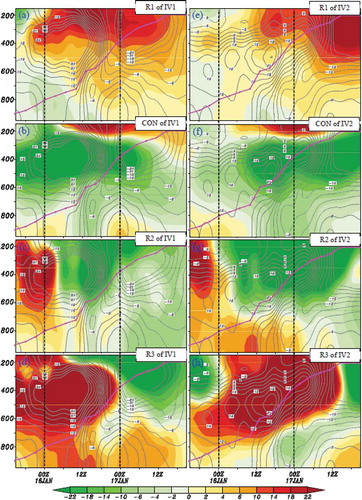
Figure 3. Budget terms of the rotational wind KE (shading; units: 10⁻³ J kg⁻¹s⁻¹) averaged within IV1 and IV2 (purple dashed boxes shown in Figure 1(a)), where the gray contours are TOT_R (units: 10⁻³ J kg⁻¹s⁻¹, with an interval of 3 × 10⁻³ J kg⁻¹s⁻¹), the solid purple line marks the top level of the cyclone, and the black-dashed lines show the maximum development stage.

Figure 4. Budget terms of the rotational wind KE (shading; units: 10⁻³ J kg⁻¹s⁻¹) averaged within IV3 and IV4 (purple dashed boxes shown in Figure 1(a)), where the gray contours are TOT_R (units: 10⁻³ J kg⁻¹s⁻¹, with an interval of 3 × 10⁻³ J kg⁻¹s⁻¹), the solid purple line marks the top level of the cyclone, and the black-dashed lines show the maximum development stage.

From Figures 3 and 4, the mechanisms accounting for the variation of lower-tropospheric rotational wind KE within different key regions can be summarized as follows. For key region IV1, the import of wind KE by the rotational wind (term R3) was the dominant factor (Figure 3(d)); the work done by pressure gradient force (term R2) had an overall weak favorable effect on the enhancement (Figure 3(c)); the work done by divergent wind (term R1) nearly showed a neutral effect (Figure 3(a)); whereas, the conversion term (term CON) mainly transferred rotational wind KE to divergent wind KE (Figure 3(b)), which decelerated the enhancement of rotational wind KE. For key region IV2, pressure gradient force’s work was the most important factor for the enhancement of rotational wind KE (Figure 3(c)); transport of wind KE by rotational wind (Figure 3(h)) and work done by divergent wind (Figure 3(e)) were also conducive to the enhancement; whereas, the conversion term mainly converted rotational wind KE to divergent wind KE (Figure 3(f)), which slowed the enhancement. For key region IV3, the import of wind KE by the rotational wind (Figure 4(d)) and work done by pressure gradient force (Figure 4(c)) governed the enhancement; work done by divergent wind (Figure 4(a)) was also favorable; whereas the conversion term (Figure 4(b)) mainly decelerated the enhancement of rotational wind KE. For key region IV4, the northward transport of wind KE by the rotational wind (Figure 4(h)) governed the enhancement; pressure gradient force did positive work first and negative work later (Figure 4(g)), which rendered a total effect of nearly zero; whereas, the work done by divergent wind (Figure 4(e)) and the conversion between rotational and divergent wind KE (Figure 4(f)) exerted an obvious negative effect, which decelerated the acceleration of rotational wind KE.

As discussed above, the most favorable and detrimental factors for the enhancement of lower-tropospheric rotational wind KE within key regions IV1–4 are summarized in Table 1. It is shown that, for key regions IV2 and IV3, which were located at lower latitudes than key regions IV1 and IV4 (Figure 1(a)), wind KE production was more important than the KE transport. The reason for the notable rotational wind KE production can be summarized as (i) the EEC mainly showed a centripetal pressure gradient force (as the cyclone was a low-pressure weather system); and (b) the rotational wind associated with the cyclone showed a cyclonic centripetal motion (as the cyclone was convergent). Points (a) and (b) resulted in a positive work on the rotational wind, as the angle between pressure gradient force and rotational wind was less than 90°. For key regions IV1 and IV4, wind KE transport was more important than the KE production. The reason for the notable wind KE transport can be summarized as: (i) around key regions IV1–4, the total wind KE mainly decreased centripetally (not shown); and (ii) the southerly wind component was significant in key regions IV1–4 (not shown), as rotational wind associated with the cyclone showed a cyclonic centripetal motion. Points (i) and (ii) resulted in a northward total wind KE transport. In all the above four key regions, the conversion term mainly acted to convert the rotational wind KE to divergent wind KE, which served as a dominant factor for maintenance of the divergent wind (not shown).

Table 1. The most favorable and detrimental factors for the enhancement of lower-tropospheric rotational wind KE within key regions IV1–IV4.

	Key region IV1	Key region IV2	Key region IV3	Key region IV4
Most favorable factors	R3	R2	R2, R3	R3
Most detrimental factors	CON	CON	CON	R1, CON

4. Conclusion

Based on a reasonable simulation of an extreme EEC that occurred over the western North Pacific Ocean during mid-January 2011 (Fu et al. 2018), this study investigated the energetics features of the EEC and determined the mechanisms accounting for the rapid enhancement of the lower-tropospheric winds associated with the cyclone by applying rotational and divergent wind KE analyses and budgets. Overall, the total wind KE associated with the EEC showed a remarkable enhancement in the lower troposphere during the maximum development stage (whereas, the middle- and upper-tropospheric total wind KE featured an unobvious variation and an obvious reduction, respectively). This was mainly due to the increase of rotational wind KE, particularly in the southeastern section of the cyclone, where the maximum surface wind appeared. The rotational wind KE enhancement was important for both the horizontal enlargement and upward stretching of the EEC. In contrast, the divergent wind KE, which was much smaller than the rotational wind, mainly featured a decreasing trend (corresponding to weakening of low-level convergence). The nonorthogonal wind KE, which linked the total wind KE, rotational wind KE, and divergent wind KE, showed obviously different relations to the rotational and divergent wind KE: in regions with strong rotational wind, it mainly enhanced the total wind KE; whereas, in regions with strong divergent wind, it mainly reduced the total wind KE.

Rotational wind KE budgets indicated that key regions IV1–4 of the EEC featured the largest lower-tropospheric rotational wind and fastest rotational wind enhancement. Within these key regions, remarkable similarities and differences could be found in the mechanisms accounting for the variation of lower-tropospheric rotational wind KE. For key regions IV1 and IV4, which were located at higher latitudes than key regions IV2–3, northward transport of total wind KE through key regions’ southern boundaries governed the rotational wind KE enhancement; for key region IV2, rotational wind KE production due to the work done by pressure gradient force was dominant; for key region IV3, mechanisms conducive to the rotational wind KE were a hybrid of the above two factors. Within key regions IV1–4, an overall conversion from rotational wind KE to divergent wind KE was obvious. This decelerated the rotational wind enhancement but served as a dominant factor for the maintenance of the divergent wind. This study provides a useful method and some new understandings of the rapid development of EECs. However, as a case study, the main findings in this work will certainly have some limitations. Therefore, more EEC events should be investigated in the future by using similar methods, so as to render a more comprehensive understanding of the wind enhancement associated with EECs.

Acknowledgments

The authors thank the National Centers for Environmental Prediction and the China Meteorological Administration for providing the data.

Disclosure statement

No potential conflict of interest was reported by the authors.

Correction Statement

This article has been republished with minor changes. These changes do not impact the academic content of the article.

Additional information

Funding

This research was supported by the National Key R&D Program of China [grant number 2018YFC0809400]; the National Natural Science Foundation of China [grant numbers 41775046 and 91637211]; and the Youth Innovation Promotion Association, Chinese Academy of Sciences.

References

- Buechler, D. E., and H. E. Fuelberg. 1986. “Budgets of Divergent and Rotational Kinetic Energy during Two Periods of Intense Convection.” Monthly Weather Review 114 (1): 95–114. doi:10.1175/1520-0493(1986)114<0095:BODARK>2.0.CO;2.
- Chen, S.-J., and L. Dell’osso. 1987. “A Numerical Case Study of East Asian Coastal Cyclogenesis.” Monthly Weather Review 115 (2): 477–487. doi:10.1175/1520-0493(1987)115<0477:ANCSOE>2.0.CO;2.
- Ding, Y., and Y. Liu. 1985. “On the Analysis of Typhoon Kinetic Energy, Part II Conversion between Divergent and Nondivergent Wind.” Science in China (B) 15 (11): 1045–1054. doi:10.1360/zb1985-15-11-1045.
- Dudhia, J. 1989. “Numerical Study of Convection Observed during the Winter Monsoon Experiment Using a Mesoscale Two-Dimensional Model.” Journal of the Atmospheric Sciences 46 (20): 3077–3107. doi:10.1175/1520-0469(1989)046<3077:NSOCOD>2.0.CO;2.
- Fu, S., F. Yu, D. Wang, and R. Xia. 2012. “A Comparison of Two Kinds of Eastward-moving Mesoscale Vortices during the Mei-yu Period of 2010.” Science China Earth Sciences 56 (2): 282–300. doi:10.1007/s11430-012-4420-5.
- Fu, S., J. Sun, and J. Sun. 2014. “Accelerating Two-stage Explosive Development of an Extratropical Cyclone over the Northwestern Pacific Ocean: A Piecewise Potential Vorticity Diagnosis.” Tellus A: Dynamic Meteorology and Oceanography 66: 1, 23210. doi:10.3402/tellusa.v66.23210.
- Fu, S., J. Sun, S. Zhao, and W. Li. 2011. “The Energy Budget of a Southwest Vortex with Heavy Rainfall over South China.” Advances in Atmospheric Sciences 28 (3): 709–724. doi:10.1007/s00376-010-0026-z.
- Fu, S., J. Sun, W. Li, and Y. Zhang. 2018. “Investigating the Mechanisms Associated with the Evolutions of Twin Extratropical Cyclones over the Northwest Pacific Ocean in Mid‐January 2011.” Journal of Geophysical Research 123 (8): 4088–4109. doi:10.1002/2017JD027852.
- Grell, G. A. 1993. “Prognostic Evaluation of Assumptions Used by Cumulus Parameterizations.” Monthly Weather Review 121 (3): 764–787. doi:10.1175/1520-0493(1993)121<0764:PEOAUB>2.0.CO;2.
- Grell, G. A., J. Dudhia, and D. R. Stauffer. 1995. A Description of the Fifth-generation Penn State/NCAR Mesoscale Model (MM5), 122. NCAR Tech. Note NCAR/TN_398_STR. doi: 10.5065/D60Z716B.
- Hakim, G. J., D. Keyser, and L. F. Bosart. 1996. “The Ohio Valley Wave-Merger Cyclogenesis Event of 25–26 January 1978. Part II: Diagnosis Using Quasigeostrophic Potential Vorticity Inversion.” Monthly Weather Review 124 (10): 2176–2205. doi:10.1175/1520-0493(1996)124<2176:TOVWMC>2.0.CO;2.
- Hawkins, H. F., and S. L. Rosenthal. 1965. “On the Computation of Stream Functions from the Wind Field.” Monthly Weather Review 93 (4): 245–252. doi:10.1175/1520-0493(1965)093<0245:OTCOSF>2.3.CO;2.
- Kuwano-Yoshida, A., and Y. Asuma. 2008. “Numerical Study of Explosively Developing Extratropical Cyclones in the Northwestern Pacific Region.” Monthly Weather Review 136 (2): 712–740. doi:10.1175/2007mwr2111.1.
- Lupo, A. R., P. J. Smith, and P. Zwack. 1992. “A Diagnosis of the Explosive Development of Two Extratropical Cyclones.” Monthly Weather Review 120 (8): 1490–1523. doi:10.1175/1520-0493(1992)120<1490:ADOTED>2.0.CO;2.
- Lynch, P. 1988. “Deducing the Wind from Vorticity and Divergence.” Monthly Weather Review 116 (1): 86–93. doi:10.1175/1520-0493(1988)116<0086:DTWFVA>2.0.CO;2.
- Qi, G.-Y. 1993. “Climatic Characteristics of Explosive Cyclone over the North Pacific Ocean.” Quarterly Journal of Applied Meteorology 4: 426–433.
- Reisner, J., R. M. Rasmussen, and R. T. Bruintjes. 1998. “Explicit Forecasting of Supercooled Liquid Water in Winter Storms Using the MM5 Mesoscale Model.” Quarterly Journal of the Royal Meteorological Society 124 (548): 1071–1107. doi:10.1002/qj.49712454804.
- Reynolds, R. W., N. A. Rayner, T. M. Smith, D. C. Stokes, and W. Wang. 2002. “An Improved in Situ and Satellite SST Analysis for Climate.” Journal of Climate 15 (13): 1609–1625. doi:10.1175/1520-0442(2002)015<1609:AIISAS>2.0.CO;2.
- Sanders, F., and J. R. Gyakum. 1980. “Synoptic-dynamic Climatology of the “Bomb”.” Monthly Weather Review 108 (10): 1589–1606. doi:10.1175/1520-0493(1980)108<1589:SDCOT>2.0.CO;2.
- Schultz, D. M., L. F. Bosart, B. A. Colle, H. C. Davies, C. Dearden, D. Keyser, and O. Martius, et al. 2019. “Extratropical Cyclones: A Century of Research on Meteorology’s Centerpiece.” Meteorological Monographs 59: 16.1-.56. doi:10.1175/amsmonographs-d-18-0015.1.
- Wu, L., J. E. Martin, and G. W. Petty. 2011. “Piecewise Potential Vorticity Diagnosis of the Development of a Polar Low over the Sea of Japan.” Tellus A: Dynamic Meteorology and Oceanography 63 (2): 198–211. doi:10.1111/j.1600-0870.2011.00511.x.
- Xu, Q., J. Cao, and S. Gao. 2011. “Computing Streamfunction and Velocity Potential in a Limited Domain of Arbitrary Shape. Part I: Theory and Integral Formulae.” Advances in Atmospheric Sciences 28 (6): 1433–1444. doi:10.1007/s00376-011-0185-6.
- Ying, M., W. Zhang, H. Yu, X. Lu, J. Feng, Y. Fan, Y. Zhu, and D. Chen. 2014. “An Overview of the China Meteorological Administration Tropical Cyclone Database.” Journal of Atmospheric and Oceanic Technology 31 (2): 287–301. doi:10.1175/JTECH-D-12-00119.1.
- Yoshida, A., and Y. Asuma. 2004. “Structures and Environment of Explosively Developing Extratropical Cyclones in the Northwestern Pacific Region.” Monthly Weather Review 132 (5): 1121–1142. doi:10.1175/1520-0493(2004)132<1121:SAEOED>2.0.CO;2.
- Zwack, P., and B. Okossi. 1986. “A New Method for Solving the Quasi-Geostrophic Omega Equation by Incorporating Surface Pressure Tendency Data.” Monthly Weather Review 114 (4): 655–666. doi:10.1175/1520-0493(1986)114<0655:ANMFST>2.0.CO;2.