A review of surface ozone source apportionment in China

ABSTRACT

Air pollution caused by particulate matter has significantly improved in China in recent years since the implementation of a series of stringent clean-air regulations. However, surface ozone concentrations have increased, especially in developed city clusters, such as the Beijing–Tianjin–Hebei, Yangtze River Delta, Pearl River Delta, and Sichuan Basin regions. Due to the complexity and nonlinearity of the ozone formation, accurately locating major sources of ozone and its precursors is an important basis for the formulation of cost-effective pollution control strategies. In this paper, the authors systematically summarize the reported results and outcomes of the methods and main conclusions of ozone source apportionment (regions and categories) in China from the published literature, based on observation-based methods and emission-based methods, respectively. The authors aim to provide a comprehensive understanding of ozone pollution and reliable references for the formulation of air pollution prevention policies in China.

GRAPHICAL ABSTRACT

摘要

近年来, 在实施了一系列较为严格的空气污染控制措施后, 中国的PM_2.5污染已得到明显改善, 但近地面臭氧污染问题却日益凸显, 尤其是在一些发达的城市群, 如京津冀, 长三角, 珠三角和四川盆地地区。鉴于臭氧生成的复杂性及其与前体物的非线性关系, 准确定位臭氧及其前体物的来源是制定经济高效的臭氧污染控制策略的重要前提。本文总结了近20年来国内外已发表文章中关于中国臭氧来源 (包括区域和行业来源) 的主要方法 (包括基于观测的方法和基于排放的方法) 和结论, 希望能为中国臭氧污染的全面了解和空气污染防治政策的制定提供可靠的参考。

KEYWORDS:

• Surface ozone
• long-term trends
• ozone source apportionment
• literature review

关键词:

• 近地面臭氧;长期趋势;臭氧来源解析;文献综述

1. Introduction

Tropospheric ozone is produced via the photochemical reaction of volatile organic compounds (VOCs), carbon monoxide (CO), and nitrogen oxides (NO_x = NO + NO₂) in the presence of sunlight (Atkinson 2000). Photochemical smog pollution was first reported in Los Angeles in 1940, but it was not until the 1950 s that Haagen-Smit (1952) determined that the irritating gas in the air was ozone (Tang, Zhang, and Shao 2006). Since then, photochemical smog pollution has emerged all over the world, but is especially serious in North America and Europe (Fiore et al. 1998; Solomon et al. 2000). Due to the continuous efforts with emissions control and restriction, ozone concentrations in most regions of the world, including North America, Europe, and North Africa, have decreased significantly in the past three decades. However, in East Asia, especially in China, ozone concentrations have shown an obvious increasing trend (Schultz et al. 2017; Gaudel et al. 2018; Lin et al. 2017).

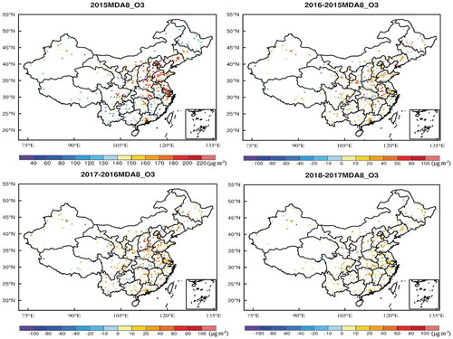
Lanzhou Xigu, a region of northwestern China with a large number of petrochemical industries, was in the late 1970s the first city in China to report field evidence of photochemical smog, which is widely regarded as a milestone of photochemical smog research and protection in China (Tang, Zhang, and Shao 2006). Over the past 20 years, serious ozone pollution has been found in the most highly populated and industrialized city clusters in China (Wang et al. 2017a, 2017b). Figure 1(a) shows that the highest levels of ozone pollution in China in recent years have been reported in the Beijing–Tianjin–Hebei (BTH), Yangtze River Delta (YRD), Pearl River Delta (PRD), and Sichuan Basin (SCB) regions. Many studies have analyzed the long-term trends of in-situ ozone field measurements and have consistently concluded that tropospheric ozone in China has been increasing since the 1990s (Xu et al. 2008a; Wang et al. 2009a; Sun et al. 2016; Wang et al. 2017a). For example, surface ozone concentrations increased at a growth rate of 1.8 ppbv yr⁻¹ at the Lin’an regional background station in Hangzhou from 1991 to 2006 (Xu et al. 2008a), and at a rate of 1.13 ppbv yr⁻¹ at Shangdianzi in Beijing from 2003 to 2015 (Ma et al. 2016). Concentrations of ozone in western China (e.g. at Waliguan) also increased, at a growth rate of 0.28 ppbv yr⁻¹ for nighttime ozone and 0.24 ppbv yr⁻¹ for daytime ozone, during the period 1994–2013 (Xu et al. 2016). Statistics for observational data from a network of 1484 sites operated by the China Ministry of Ecology and Environment (available at http://106.37.208.233:20035/) indicate that the 90th percentile of the daily maximum 8-h average ozone concentration (MDA8_O₃) at most stations in highly polluted areas had a significantly increasing trend from 2015 to 2018, although there was a slowdown in the growth rate in 2018 as a result of strict emission reduction measures (Figure 1).

Figure 1. The 90th percentile of annual MDA8_O₃ in (a) 2015 and the difference values during (b) 2015–16, (c) 2016–17, and (d) 2017–18 at the network of 1484 sites operated by the China Ministry of Ecology and Environment.

Figure 2 shows the annual variation in the number of sites at which the value of the 90th percentile of MDA8_O₃ exceeded the national secondary air quality standard of 160 µg m⁻³ and the annual maximum MDA8_O₃ (not for the same site in each of these four years) based on monitoring results from 1484 sites in the period 2015–18. The number of sites exceeding these thresholds increased from 424 (28.6%) sites in 2015 to 636 (45.7%) sites in 2018. The annual maximum MDA8_O₃ also increased, from 226.8 µg m⁻³ in 2015 to 238 µg m⁻³ in 2017, but it experienced a small decrease in 2018, which may reflect the significant achievements made in the implementation of emission reduction policies focused on VOCs control since 2018 (State Council 2018; Ou et al. 2016). Increased concentrations of tropospheric ozone have a detrimental effect on both human health and crop production (Feng et al. 2015; Wang et al. 2017a).

Figure 2. Interannual variations in the number of sites at which the value of the 90th percentile of MDA8_O₃ exceeded the national secondary air quality standard 160 µg m⁻³ (NSE) and the annual maximum MAD8_O₃ (MAX, not for the same site in each of these four years) based on the monitoring results from 1484 sites operated by the China Ministry of Ecology and Environment over 2015–18. The values above the bars represent the annual percentage of sites where the national secondary air quality standard was exceeded and the values of annual maximum MAD8_O₃, respectively.

The control of ozone pollution is a great challenge because of the diverse range of precursors and the nonlinear relationship between ozone concentrations and these precursors (Xing et al. 2011). Previous studies have suggested that increased amounts of anthropogenic non-methane VOCs have dominated the increase in ozone over eastern China (Sun et al. 2019) and that previous control measures focusing only on NO_x may not work or may even aggravate ozone pollution in the city clusters (Tang et al. 2012; Gao et al. 2017a; Wang et al. 2019a). Owing to the relatively long lifetime of ozone in the troposphere (Lin, Wuebbles, and Liang 2008), which may be as high as several days to weeks, high levels of ozone pollution are not only derived from local emission sources, but also from regional and even super-regional (outside the simulated area) transport (Zheng et al. 2010; Wang et al. 2011). Accurately determining the main sources of ozone (including the source regions and source categories) is therefore the key to the formulation of a reasonable and efficient ozone control strategy. In addition, several recent studies have proposed that the rapid decrease in PM_2.5 concentrations may have been an important factor in the increase in ozone pollution in China (Li et al. 2018a, 2019a, 2019b), which demonstrates the complexity of ozone pollution control and the urgent need for a win-win control strategy.

This paper is arranged as follows: Section 2 lists the approaches and main conclusions of studies on the sources of ozone and its precursors for both regional and sectoral sources in China, including back-trajectory analyses and ozone source apportionment based on the observation-based method (OBM) and emissions-based method (EBM). Section 3 provides a summary and some discussion for future research and the formulation of control strategies for ozone pollution.

2. Ozone source apportionment

An accurate analysis of the regional and sectoral sources of surface ozone is the most important prerequisite for the development of cost-effective ozone control policies. The trajectories of air masses have been widely studied in China to analyze the source and transport characteristics of ground-level ozone (Wang et al. 2006; Zheng et al. 2010; Liu et al. 2016a). However, this approach only analyzes the physical transport and deposition processes without taking into consideration the chemical processes, so it is more suitable for primary pollutants than secondary pollutants. Ozone formation is a secondary process and has a nonlinear response to the precursor chemicals (Sillman 1999; Zhang et al. 2008). Therefore, ozone source apportionment is required to determine the relative importance of NO_x and VOC emissions from different sectors and source regions.

Two methods are commonly used to study ozone sources: the EBM and the OBM (Russell and Dennis 2000). Table 1 gives a brief summary of the advantages and disadvantages of these two methods. Based on a known emissions inventory, the EBM can predict the transport and photochemical reactions of ozone and its precursors by performing numerical simulations based on air quality models. The OBM simulates the processes of atmospheric photochemical pollution constrained by measurements of the concentrations of ozone, NO₂, CO, HONO, and VOCs, the photolysis rate constant, temperature, humidity, and pressure. Compared with the EBM, the OBM can avoid the uncertainties caused by emission inventories and the simulated dynamics of the boundary layer (Russell and Dennis 2000), which has significant advantages for China because of the relatively insufficient research on emission inventories. As a result of the limitations of high-quality observational data, however, ozone source apportionment based on the OBM is limited to the study of fixed time and sites in practical applications and the regional sources of ozone cannot be analyzed. Therefore, the OBM should be viewed as a complement to, rather than a substitute for, the EBM.

Table 1. Brief summary of the advantages and disadvantages of ozone source apportionment methods.

Methodology	Advantages	Disadvantages	Methodology	Advantages	Disadvantages
Back-trajectory analysis	Simple principle and easy to operate. Can give the possible origin and transport trajectory.	Only transport and deposition process; lack of chemical reactions. Cannot accurately locate and quantify the contributions.
OBM	No need to input emission inventories.	High requirements for the accuracy and representativeness of the observation data. Limited to fixed time and sites. Only chemical reactions; lack of transport process.	CMB	Non-strict requirements on the number of ambient samples.	Requirements for accurate source profiles (Watson, Chow, and Fujita 2001). Collinearity of similar sources (Y J, Zheng, and Cai et al. 2015).
			PMF	No need to input the source profiles. Non-negative constraint can avoid negative contributions (Paatero 2004).	Need a lot of observation samples (Y J, Zheng, and Cai et al. 2015). Complicated and time-consuming.
EBM	Can simulate all the atmospheric physical and chemical processes during the whole simulated period.	Uncertainty of emission inventories	Sensitivity analysis	Simple and convenient to implement. Quantify the response of O3 concentrations to changes in the precursor emissions (Russell and Dennis 2000).	Large computation. The results include the effects of nonlinearity (Dunker et al. 2002; Qu et al. 2014; Clappier et al. 2017). Results include both positive and negative sensitivities (Zhang, Vijayaraghavan, and Seigneur 2005).
			Tagged source technology	Mass-balance of pollutants and eliminate nonlinear errors (Zhang, Vijayaraghavan, and Seigneur 2005; Kwok et al. 2015). Simultaneous calculation of concentration; sensitivity and contributions of different source categories in a single simulation (Kwok et al. 2015). Always predicts positive contributions (Zhang, Vijayaraghavan, and Seigneur 2005).	Unable to calculate emissions reduction percentage and predict the effects of emission reductions.

2.1 Back-trajectory analysis

The Hybrid Single Particle Lagrangian Integrated Trajectory (HYSPLIT) model (http://ready.arl.noaa.gov/HYSPLIT.php)—a mixed model using both the Eulerian and Lagrangian methods—is a useful tool for calculating back-trajectories. The accuracy of an individual trajectory is limited by the temporal and spatial resolution of the meteorological observations, measurement errors, numerical errors, and by the simplifying assumptions used in the trajectory model (Moody et al. 1995; Kahl 1996). Therefore, cluster analysis is often performed with a large number of back-trajectories to overcome these uncertainties and limitations. For example, Wang et al. (2006) concluded that ozone and its precursors from eastern central China and the YRD region may contribute to the high concentrations of ozone observed at Mount Tai and Huang through back-trajectory analysis. Although the back-trajectory method has been used to analyze the importance of regional transport for local ozone concentrations in many previous studies in China (Zheng et al. 2010; Liu et al. 2016a), it can only give a rough picture of the origin and transport pathways of large-scale air masses and cannot accurately locate and quantify the contributions, as shown in Table 1. This method is commonly used as a pilot analysis for regional sources and needs to be further explored in conjunction with other source attribution methods.

2.2 Ozone source apportionment based on OBMs

2.2.1 Receptor model

Previous studies have found that the increasing trend of ground-level ozone concentrations is related to high levels of anthropogenic emissions of VOCs and that the production of ozone is VOCs-limited in the urban areas of China (Liu et al. 2010; Su et al. 2017; Tang et al. 2017). Therefore, the identification and quantification of the sources of VOC emissions and their relationship with ozone production are a prerequisite for formulating an effective strategy for controlling ozone pollution. VOCs are usually attributed to a particular source using receptor models such as the chemical mass balance (CMB) and positive matrix factorization (PMF) methods based on the observed chemical composition. The mathematical and physical basis of CMB and PMF are both mass-balance Equations:

(1) $X=GF+E,$(1)

where X represents the concentration of chemical species at a given receptor site, G represents the contribution of the source to the acceptor site, F represents the mass fraction of the chemical species in the source (that is, the source component spectrum), and E is the residual. The physical basis of this equation is that the ambient concentration of a chemical species is equal to the linear sum of the product of the source contribution concentration value and the mass fraction of the species in the source composition spectrum.

Both methods are solved by the least-squares method. In contrast, the CMB method needs to input the source spectrum information (F) and the ambient concentration (X) at the receptor site, so the source contribution (G) is solved, while the PMF method only needs to input the ambient concentration (X), then solve the source contribution (G) and source spectrum information (F) (Song et al. 2008; Zhang et al. 2015). For a detailed introduction to solving this equation, please refer to Paatero (2004) and Song et al. (2007). For example, Song et al. (2007) used the CMB model to apportion the contributions of VOC sources and identified eight major sources of VOCs in Beijing. Guo et al. (2011) conducted source apportionment using the PMF method in the PRD region, identifying five and six emission sources of VOCs in Hong Kong and the inland region of the PRD, respectively. They also suggested that vehicular emissions and solvent use were the major sources of VOCs in the PRD (including Hong Kong) region.

Table 2 summarizes previous studies on the source apportionment of VOCs in four highly developed city clusters in China using these two receptor models during the past decade. Most of the work has been conducted in the BTH, YRD, and PRD regions, with only a few studies in the SCB region. Table 2 also lists the top three sources of VOCs in these studies, which suggests that vehicle exhausts, solvent use, liquefied petroleum gas, and the petrochemicals industry were the dominant sources of ambient VOCs in China. However, due to differences in the dominant industrial structure, the major sources differed in four clusters. Gasoline-related emissions (a combination of vehicle exhaust fumes and gasoline vapor), industrial emissions, and liquefied petroleum gas were the prominent sources of VOCs in the BTH region as a result of the large number of gasoline-powered vehicles and factories in Tianjin and Hebei. By contrast, the proportion of biomass burning increased in the YRD and PRD regions (up to 24%) due to the uncontrolled burning of straw residues from crops. The contributions of solvent usage in the PRD region (up to 51%) were larger than those in other regions, which may be attributable to the high-speed development of manufacturing and other industrial construction in the PRD region. The contribution of natural sources of VOCs from the dense vegetation in the SCB region (up to 14%) is significantly higher than in the other regions.

Table 2. Summary of CMB and PMF studies on the source apportionment of VOCs over China.

Region	Receptor	Period	Method	Top three major sources	Reference
BTH	Beijing	2002–03	CMB	Vehicle exhaust (57.7%), painting (12.4%), gasoline vapor (11.3%)	Liu et al. (2005)
	Beijing	Aug 2005	CMB	Gasoline exhaust (47%), LPG^a (26%), petrochemicals (10%)	Song et al. (2008)
	Beijing	Aug 2005	PMF	Gasoline related (52%), petrochemicals (20%), LPG(11%)	Song et al. (2007)
	Beijing (urban)	15 Aug–10 Sep 2006	PMF	Vehicle-related (62%), paint and industrial coating (16%), LPG (13%)	Yuan et al. (2009)
	Beijing (rural)			Vehicle-related (38%), LPG (37%), paint and industrial coating (14%)
	Tianjin	6–14 Aug 2009	PMF	Vehicle-related (51%), industry-related (26%), biogenic emission (9.5%)	Han et al. (2015)
	Beijing	18 Oct–22 Nov 2014	PMF	Fuel combustion (27%), vehicle exhaust (22%), solvent usage (10%)	Li et al. (2015a)
	Beijing	Nov 2014	PMF	Vehicle exhaust (41.4%), gasoline vapors and industrial production (33.4%), LPG/NG^b (25.3)	Wang et al. (2016)
	Tianjin	Nov 2014–Oct 2015	PMF	Automobile exhaust (23.1%), industry emission (19.9%), LPG/NG (18.6%)	Liu et al. (2016b)
	Beijing	11 Aug–3 Sep 2015	PMF	Vehicular exhaust (28%–33%), gasoline evaporation and exhaust (17%–24%), fuel combustion (10%–13%)	Li et al. (2016a)
	Langfang	Apr 2016–Mar 2017	PMF	Vehicular emissions (44.8%), LPG/NG/combustion (24.9%), petrochemical industry (9.6%)	Song et al. (2019a)
	Xianghe	6 Nov 2017–29 Jan 2018	PMF	Vehicle exhaust (31.0%), industrial emissions (26.4%), LPG/NG (18.6%)	Yang et al. (2019a)
YRD	Shanghai	2007–10	PMF	Solvent usage (32%), vehicle related (25%), fuel evaporation (15%)	Cai et al. (2010)
	Shanghai	Jan 2009–Dec 2010	PMF	Vehicular emissions (27.6%), coal burning and regional transport (24.9%), solvent usage (19.4%)	Wang et al. (2013)
	Ningbo	Dec 2012–Oct 2013	PMF	Petrochemical industry (35.6%), fuel and evaporation (16%), vehicle emissions(15.6%)	Mo et al. (2017)
	Nanjing	15 May–31 Aug 2013	PMF	Industry-related (52%), vehicular emission (34%), LPG/NG (9%)	Shao et al. (2016)
	Nanjing	Aug–Sep 2013	PMF	Vehicular emissions (38%), LPG/NG (20%), solvent usage (19%)	An et al. (2017)
		Dec 2013–Feb 2014		LPG/NG (36%), vehicular emissions (30%), biomass/biofuel burning (18%)
	Nantong	30 Jul–1 Aug 2014	PMF	Solvent use (16.2%), NG (15.6%), LPG (13.9)	Zhang et al. (2018)
	MLYR^c	22 Nov–4 Dec 2015	PMF	Combustion-related emissions (36.1%), regional aged air mass (27.5%), shipping emissions (23.5%)	Zhu et al. (2018)
	Shanghai	24 Aug–15 Sep 2016	PMF	Petrochemical industry (22.1%–33.9%), vehicle exhaust (22.2%–27.3%), solvent use (15.0%–20.1%)	Zheng et al. (2019)
	Shanghai	20–30 May 2017	PMF	Vehicle exhaust (33.9%), solvent use (22.6%), aged air mass and secondary formation (22.1%)	Liu et al. (2019b)
PRD (including Hong Kong)	Guangzhou	Oct–Nov 2004	CMB	Vehicle exhaust (31%–53%), solvent use (16%–44%), LPG (5%–16%)	Liu et al. (2008)
	Guangzhou	23 Oct–1 Dec 2007	PMF	Solvent usage (51%), vehicular emissions (19%), biomass burning (12%)	Ling et al. (2011)
	Hong Kong	Sep 2002–Aug 2003	PMF	LPG (22.5%), vehicle and marine vessel exhausts (19.8%), consumer and household products (9.1%)	Lau et al. (2010)
		Sep 2006–Aug 2007		LPG (31.3%), vehicle and marine vessel exhausts (17.9%), consumer and household products (8.88%)
	Guangzhou	Oct–Dec 2007	PMF	Solvent usage (46%), vehicular emission (26%), biomass burning (11%)	Guo et al. (2011)
	Hong Kong			Vehicular emission (48%), solvent usage (43%), biomass burning (9%)
	PRD	2005–08	PMF	Vehicular emissions (25%), industrial sources (17%), paint solvent use (17%)	Wu et al. (2016)
	PRD	Summer, winter 2008–09	PMF	Gasoline exhaust (23%), industrial emissions (16%), LPG and propellant emission (13%)	Yuan et al. (2013)
	Hong Kong	2005–10	PMF	Solvent usage (41%), vehicular emissions (31%), gasoline vapor and LPG usage (22%)	Ling et al. (2013)
	Hong Kong	6 Sep–29 Nov 2010	PMF	Vehicle exhaust (42%), solvent related sources (25%), gasoline (22%)	Ling and Guo (2014)
	Hong Kong	30 Oct–3 Nov 2010	PMF	LPG and consumer products (20%), diesel vehicular (18%), gasoline evapor (17%)	Lam et al. (2013)
	Hong Kong	2005–13	PMF	Consumer product and painting (32.6%), gasoline evapor and LPG (25.4%), architectural paints (21.5%)	Ou et al. (2015)
	Heshan	22 Oct–20 Nov 2014	PMF	Vehicular emissions (58%), biomass burning (24%), solvent usage (18%)	He et al. (2019)
	Heshan	22 Oct–22 Nov 2014	PMF	Vehicle exhaust (20%), paint solvent usage and LPG usage (22%), coal burning and industrial combustion sources (17%)	Song et al. (2019b)
SCB	Sichuan	2008–11	PMF	Gasoline-related emission (35%), fuel combustion (29%), solvent use (22%)	Zhang et al. (2014)
	Chongqing (rural)	24 Aug–22 Sep 2015	PMF	Aged background air (68.5%), industrial process (11.9%), biogenic (9.3%)	Li et al. (2018b)
	Chongqing (urban)			Vehicle exhaust (34.3), secondary anthropogenic (23.5%), solvent use (13%)
	Chongqing (suburban)			Vehicle exhaust (26.6%), solvent use (23.7%), secondary anthropogenic (22.4%)

Note: ^aLPG is liquefied petroleum gas.

^bNG is natural gas.

^cMLYR represents the middle and lower Yangtze River.

The strengths and weaknesses of the CMB and PMF methods are also listed in Table 1. Although the PMF model can extract source contributions from ambient samples without source profiles, it also requires a lot of observational data to achieve a convergent solution and is complex and time-consuming to run. The CMB model has no strict requirement on the number of ambient samples, but requires accurate source profiles, which have a high timeliness and are location-specific (Watson, Chow, and Fujita 2001), and the actual number of sources and profiles has to be assumed in advance (Lau et al. 2010). These two methods both have very high requirements for the accuracy and representativeness of observational data and are therefore limited in practical applications.

2.2.2 Other methods based on OBMs

To better identify the contribution of VOC sources to ozone pollution, it is also necessary to understand the contributions of the VOC sources to ozone production, which are characterized by the VOC reactivity (Ran et al. 2009; Tie et al. 2009). At present, a propylene-equivalent concentration method (Chameides et al. 1992) and a maximum incremental reactivity method (Carter 1994) are widely used to calculate the reactivity of VOCs, and thus the contributions of chemical species and emission sources to the production of ozone are also evaluated (Ran et al. 2011; Li et al. 2015b; Wang et al. 2016; An et al. 2017). For instance, Yuan et al. (2009), using the PMF and maximum incremental reactivity methods, showed that vehicular activities contributed 62% to the VOC loading and 55% to the ozone formation potential (OFP) at Peking University (an urban site), but only 38% to the VOC loading and 42% to the OFP at Yufa (a rural site). Li et al. (2015b) also found that alkenes and aromatic compounds were the largest contributors (47.65%–61.53%) to the total OFP of measured VOCs in the BTH region, consistent with the results of Wang et al. (2016). However, these two methods simply estimate the amount of ozone formed under optimum or ideal conditions, which is different from the amount formed in the real atmosphere. A combination of the PMF method and the photochemical box model is a useful tool to investigate the contributions of different sources of VOCs to the formation of ozone and the major species present in the different sources (Ling et al. 2011; Ling and Guo 2014).

The relative incremental reactivity (RIR) is an important indicator estimated by the OBM to evaluate the contributions of different sources to the photochemical production of ozone. According to Carter and Atkinson (1989), the RIR of the main primary pollutants can be calculated by Equation (2)(2) $\mathrm{R}\mathrm{I}\mathrm{R}\left(Y\right)=\left[\frac{\mathrm{\Delta }{P}_{{\mathrm{O}}_3}\left(Y\right)/P_{{\mathrm{O}}_3}\left(Y\right)}{\mathrm{\Delta }S\left(Y\right)/S\left(Y\right)}\right],$(2) :

(2) $\mathrm{R}\mathrm{I}\mathrm{R}\left(Y\right)=\left[\frac{\mathrm{\Delta }{P}_{{\mathrm{O}}_3}\left(Y\right)/P_{{\mathrm{O}}_3}\left(Y\right)}{\mathrm{\Delta }S\left(Y\right)/S\left(Y\right)}\right],$(2)

where Y represents a specific hydrocarbon species, NO or CO, and $P_{{\mathrm{O}}_3}\left(Y\right)$ represents the OFP, which is the net amount of ozone produced and NO consumed during the evaluation period. $S\left(Y\right)$, which is called the source effect, represents the integrated amount of species Y emitted or transported to the measurement site that results in the concentration of Y. $\mathrm{\Delta }S\left(Y\right)$ is the hypothetical change in the source effect $S\left(Y\right)$. $\mathrm{\Delta }{P}_{{\mathrm{O}}_3}$ is therefore the change in $P_{{\mathrm{O}}_3}\left(Y\right)$ caused by the source effect change $\mathrm{\Delta }S\left(Y\right)$. RIR(Y) represents the RIR of species Y. A positive value of the RIR indicates that reducing the precursor emissions will reduce the production of ozone and, the larger the value of the RIR, the more sensitive the production of ozone is to the precursor. Conversely, a negative value of the RIR means that reducing the precursor emissions can cause an increase in ozone production (such as the NO titration effect).

Based on the OBM model, numerous studies have analyzed the RIR to evaluate the contributions of different sources (even specific VOC species) to ozone production. For example, Ling et al. (2011) applied this approach in the PRD region and reported that solvent use (51%) and vehicular emissions (19%) were the two major contributors to local VOCs. The summed RIR values of these two sources accounted for 51% and 28% of the total RIR, respectively, and, among the major sources, alkenes and most aromatic compounds, especially ethene, toluene, and m/p-xylene, were significant contributors to the formation of ozone. Meanwhile, dispersion models including the conditional probability function, the potential source contribution function, and the concentration-weighted trajectory, have also been employed to identify the geographic origins of VOCs based on PMF source contributions and the wind direction data (Song et al. 2007, 2019b; Liu et al. 2016b, 2019b).

2.3 Ozone source apportionment based on EBMs

2.3.1 Sensitivity analysis and process analysis

Sensitivity analysis, such as the brute-force method (BFM) (Sillman 1995; Wang et al. 2019a), the decoupled direct method (DDM) (Dunker et al. 2002; Chang et al. 2016), and the high-order DDM (HDDM) (Hakami, Odman, and Russell 2003; Shen et al. 2015), which can obtain the response of ozone production to the perturbed emission inventories of precursors by multiple simulation cases, are commonly used for ozone source apportionment. For example, based on the BFM using the Models-3/Community Multiscale Air Quality (CMAQ) modeling system, Streets et al. (2007) suggested that during high ozone pollution episodes, 35%–60% of the ozone in Beijing can be attributed to sources outside Beijing, with maximum contributions of 28% from neighboring Hebei Province. Feng et al. (2016) and Li et al. (2017) analyzed the contributions of different anthropogenic sources through sensitivity studies and concluded that industrial emissions played the most important role in severe ozone pollution in both Xi’an and eastern China.

The main advantage of the BFM is simplicity and convenience in implementation, but it requires relatively large changes in emissions to ensure that the response of ozone is larger than the numerical error and needs large computation resources because of the additional simulations required for each perturbation. The DDM has typically been used in photochemical grid models to calculate the first-order sensitivities with respect to emissions and the initial and boundary concentrations (Dunker et al. 2002; Yarwood et al. 2013). However, the DDM is not suitable for the nonlinear response of ozone and secondary aerosols when the fluctuations of emissions are large. Thus, the HDDM was developed by Hakami, Odman, and Russell (2003) to efficiently calculate second- and higher-order sensitivities. However, there is still a lot of uncertainty in the sensitivity analysis method due to the nonlinearity.

Process analysis, such as the integrated process rate analysis method in CMAQ (Byun and Schere 2006), is undertaken to isolate the dominant processes contributing to the formation of ozone from gas-phase chemical reactions, horizontal and vertical convection, horizontal and vertical diffusion, dry deposition, and cloud processes. Numerous process analyses have shown that regional transport processes (including horizontal and vertical transport) and chemical production are the main causes of high ozone pollution in China (Wang et al. 2006; Xu et al. 2008b; Gao and Zhang 2012). In some regions with high emissions of NO_x, such as the YRD and North China Plain (NCP), chemistry is an important sink for ozone in the surface layer and makes a significant positive contribution in the upper boundary layer, leading to the strong vertical transport of ozone from upper levels to the surface layer (Li et al. 2012a; Tang et al. 2017).

2.3.2 Tagged source technology

To achieve the mass balance of pollutants and eliminate nonlinear errors, tagged source technology has been designed to assess the source apportionment of ozone and its precursors for regions or source groups selected simultaneously within a single simulation, instead of multiple runs with the BFM. The contributions of ozone and precursor species from the initial and boundary concentrations can also be tracked as separate source groupings so that all of the contributions to ozone can be accounted for in the apportionment. Ozone Source Apportionment Technology (OSAT) (Yarwood et al. 1996) applied in the Comprehensive Air Quality Model with Extensions (CAMx) (ENVIRON 2018) is the approach most commonly used to attribute ozone sources (Wang et al. 2009b; Li et al. 2012b, 2013; Shen et al. 2015). For example, Wang et al. (2009b) applied CAMx-OSAT to simulate a heavy ozone pollution episode in Beijing and found that the elevated ozone levels in urban areas were mainly sourced from local precursor emissions (accounting for 46%), whereas those at Dingling, a regional site, were affected by plumes from the Beijing urban area (55%). Taking into consideration the fact that the location of ozone formation may not be where the precursors were emitted, Wang et al. (2009b) used the Geographic Ozone Assessment Technology to trace the formation of ozone based on the geographical location and revealed that the transport of ozone was responsible for about 70% of the regional contribution of ozone to urban areas in Beijing, whereas the transport of ozone precursors accounted for the remainder of the ozone.

Other tagged source methods are widely used in photochemical grid models—for example, the Integrated Source Apportionment Method (ISAM) coupled with the CMAQ model (Collet et al. 2018; Han et al. 2018; Liu et al. 2019a). The CMAQ-ISAM, the implementation of which builds on and improves the structure developed for Tagged Species Source Apportionment (Wang, Chien, and Tonnesen 2009c), was first applied in the source apportionment of PM_2.5 by Kwok, Napelenok, and Baker (2013) and then extended for ozone source apportionment to track the contribution from user-selected categories of NO_x and VOC emissions (Kwok et al. 2015). Han et al. (2018) and Liu et al. (2019a) apportioned the high ozone episodes in the NCP through CMAQ-ISAM and suggested that the sources of emissions in Shandong and Hebei provinces contributed the most to ozone production in the NCP. Online tagged tracer modules implemented in the NAQPMS (Li et al. 2008; Wang et al. 2008; Yang et al. 2019b) and WRF-Chem (Gao et al. 2016, 2017b) models were also applied to explore the contributions of different source regions and source categories to the concentration of ozone in China and East Asia.

Tables 3 and 4 summarize the results of ozone source apportionment over China (limited to the BTH, YRD, PRD, and SCB regions) for regional and sectoral sources, respectively, based on the EBM method. It is found that, apart from contributions from the local and surrounding areas, super-regional transport also makes a significant contribution (up to 81.5%) to the high concentrations of ozone in China. Mobile and industrial sources are the major sources of surface ozone, which is partly consistent with the results of VOC source apportionment based on the OBM in Table 2.

Table 3. Summary of ozone regional source apportionments based on EBMs over China.

Region	Period	Model/Method	Receptor	Conclusion	Reference
BTH	26 Jun–2 Jul 2000	CAMx-OSAT	Beijing (urban)	Beijing (46%), Hebei (18.9%), super-region (21.2%)	Wang, Chien, and Tonnesen (2009c)
			Beijing (Dingling)	Beijing urban areas (55.2%), Hebei (12.1%), super-region (13.9%)
	Jul 2001	CMAQ-BFM	Beijing	Regional sources (including Hebei, Tianjin, Shandong, Shanxi, 35%–60%), Hebei (10%–30%)	Streets et al. (2007)
	Aug 2008	NAQPMS-online tagged tracer method	Beijing (urabn)	Beijing (39.2%), Baoding (9.4%), Langfang (4.1%), Zhangjiakou (3.1%)	Wang et al. (2008)
			Beijing (suburban)	Beijing (41.7%), Baoding (30.8%), Langfang (11%), Tiajin (8.1%)
	11–14 Aug 2015	CAMx-OSAT	Beijing	Beijing (37%), Hebei (26%), Shandong (12%), Henan (7%)	Jia et al. (2017)
			Tianjin	Tianjin (30%), Hebei (27%), Shandong (16%), Beijing (6%)
	Jun 2015	CMAQ-ISAM	Beijing	Beijing (23.1%), Tianjin (5.3%), Hebei (35.2%), Shandong (13.2%), Shanxi (5.4%)	Han et al. (2018)
			Tianjin	Tianjin (14.9%), Hebei (29.0%), Beijing (9.0%), Shandong (37.3%), Shanxi (3.6%)
			Hebei	Hebei (36.6%), Beijing (6.3%), Tianjin (5.3%), Shandong (19.4%), Shanxi (7.7%)
	Jul 2015	CAMx-OSAT	BTH	Local sources (6.9%–19.7%), in-region sources (10.3%–32.2%), out-region sources (37.3%–60.7%), BC (14.4%–23.1%)	Wang et al. (2017c)
	1–2 Jul 2015	CMAQ-ISAM	Beijing	Beijing (6.5%), Hebei (9.5%), BC (77.5%)	Liu et al. (2019a)
	3–10 Jul 2015			Beijing (13.6%), Tianjin (9.6%), Hebei (19.0%), Shandong (13.0%), BC (31.6%)
YRD	23–25 May 2004	NAQPMS-BFM	Mt. Tai and Mt. Huang	PRD regions and East China sources (20%–50%)	Wang et al. (2006)
	Jun 2006	NAQPMS-online tagged tracer method	Mt Tai	Local (11.5%), southern Shandong (21.5%), Jiangsu (9.8%), Anhui (6.6%), super-region (39.7%)	Li et al. (2008)
	6–31 Aug 2010	CAMx-OSAT	Shanghai	Shanghai (22.8%), Zhejiang (8.6%), Jiangsu (7.4%), super-region (61.2%)	Wang et al. (2014)
	9–30 Jun 2011	WRF-Chem-online tagged tracer method	Mt.Huang	Jiangxi (9.9%), regional sources (41.6%), super-region (55.4%)	Gao et al. (2017b)
	10–26 May 2013 (westerly^b)	WRF-Chem-online tagged tracer method	YRD	YRD (15%), Anhui (16.2%), Shandong (13.6%), Henan & Hebei (9%), super-region (35%)	Gao et al. (2016)
	~ (southerly)			YRD (27.9%), Anhui (12.8%), southern Zhejiang (8.2%), Hebei & Henan (6.2%), super-region (33.5%)
	~ (easterly)			YRD (31.3%), southern Zhejiang (7.3%), super-region (52.3%)
	Jul 2013	CAMx-OSAT	Shanghai	Shanghai (16%), Zhejiang (41.7%), Anuhui (19.1%), Jiangsu (4.4%), super-region (18.8%),	Li et al. (2016b)
			Chongming	Anuhui (28.2%), Zhejiang (25.5%), Jiangsu (16.2%), Shanghai (15.6%), super-region (14.5%)
			Dianshan Lake	Zhejiang (48.5%), Jiangsu (11.7%), Anhui (11.6%), Shanghai (7.4%), super-region (20.9%)
	Aug 2015	CAMx-OSAT	Shanghai	Shanghai (11.4%), northern Zhejiang (12.4%), southern Jiangsu (6.2%), super-region (50%)	Li et al. (2019c)
			Nanjing	Nanjing (8%), southern Jiangsu (13%), Anhui (11%)
			Hangzhou	Hangzhou (15.5%), northern Zhejiang (12.4%)
PRD	Jan, Apr 2006	CAMx-OSAT	PRD	Local and regional sources (18.5%–31.8%), super-region (68.2%–81.5%)	Li et al. (2013)
	Jul 2006			Local and regional sources (67.7%–79.6%), super-region (20.4%–32.3%)
	Oct 2006			Local and regional sources (34.6%–55.1%), super-region (44.9%–65.4%)
	24–25 Jul 2006	CAMx-OSAT	PRD	Local (28%), regional (42%), super-region (30%)	Li et al. (2012b)
	9–10 Nov 2006			Local (13%), regional (28%), super-region (55%)
	2015	NAQPMS-online tagged tracer method	Guangzhou	Guangzhou (14%–27%), Foshan (5%–19%), northern Guangdong (9%–19%), Jiangxi (7%–22%)	Yang et al. (2019b)

Note: ^aSuper-regional sources represent the contributions of emission sources outside the simulated region to the ozone at the receptor site

^bWesterly indicates the ozone source apportionment results when the prevailing wind direction is westerly during 10–26 May 2013, as well as southerly and easterly.

Table 4. Summary of ozone sectoral source apportionments based on EBMs over China.

Region	Period	Model/Method	Receptor	Conclusions	Reference
BTH	26 Jun–2 Jul 2000	CAMx-OSAT	Beijing	Mobile sources (31.6%), industrial area sources and point sources (20%), evaporation loss (13%), biogenic sources (12%)	Wang, Chien, and Tonnesen (2009c)
	Aug 2013	CMAQ-ISAM	Beijing	Industry (35.5%), residential (2.7%), Transportation (25.7%), Power (11.9%)	Wang et al. (2019b)
YRD	6–31 Aug 2010	CAMx-OSAT	Shanghai	Industrial process (53%), vehicle emission (19%), volatile sources (13.3%)	Wang et al. (2014)
	Jul 2013	CAMx-OSAT	Shanghai	Biogenic (22.9%), industrial boilers and kilns (20.2%), transportation (15.2%), industrial process (14.9%)	Li et al. (2016b)
			Chongming	Industrial boilers and kilns (30%), biogenic (21.3%), transportation (14.7%), industrial process (9.8%)
			Dianshan Lake	Biogenic (22.9%), industrial process (20.6%), transportation (14.8%), industrial process (12.1%)
	Aug 2013	CMAQ-ISAM	Shanghai	Industry (46.6%), power (11.5%), transportation (11.1%), residential (1.2%),	Wang et al. (2019b)
	Aug 2015	CAMx-OSAT	Shanghai	Mobile sources (42.5%), stationary combustion sources (20.5%), manufacturing process sources (17.8%), biogenic emissions (14%)	Li et al. (2019c)
			Nanjing	Mobile sources (35.5%), manufacturing process sources (23.5%), stationary combustion sources (20.5%),
			Hangzhou	Mobile sources (45.6%), stationary combustion sources (24%), manufacturing process sources (15.6%)
PRD	24–25 Jul 2006	CAMx-OSAT	PRD	Mobile sources (30%), area and point sources (28%), biogenic sources (8%)	Li et al. (2012b)
	7–10 Nov 2006			Mobile sourecs (28%), area and point sources (19%), biogenic sources (8%)
	Jul 2006	CAMx-OSAT	PRD	Mobile sources (28.4%–33.8%), point sources (22.4%–27%), area sources (22.1%–22.4%)	Li et al. (2013)
	Oct 2006			Mobile sources (40%–41.6%), area sources (15.7%–22.1%), point sources (10.2%–18.3%)
	Aug 2013	CMAQ-ISAM	Guangdong	Industry (29.1%), power (18.1%), residential (2.8%), transportation (11.1%)	Wang et al. (2019b)
	2015	NAQPMS-online tagged tracer method	Guangzhou	Transportation (38%–40%), industrial (20%–24%), biogenic (7%–13%), residential (7%–14%)	Yang et al. (2019b)
SCB	Aug 2013	CMAQ-ISAM	Chongqing	Industry (32.2%), transportation (22.3%), power (13%), residential (3.5%)	Wang et al. (2019b)

We explored the differences and connections between the two ozone source apportionment methods (sensitivity analysis and tagged source technology), as shown in Table 1. The source sensitivity approach includes the effects of nonlinearity in the system because the sum of the sensitivities of all the sources is not necessarily equal to the sum of their contributions in a fluctuation-free environment (Qu et al. 2014; Clappier et al. 2017). Therefore, when the relationship between emissions and concentrations is linear, the results of these two approaches are equivalent (or close) (Baker and Kelly 2014). However, in nonlinear situations (e.g. ozone chemistry), the two approaches can provide different results and tagged species techniques have the advantage of providing accurate source apportionments for nonlinear systems (Zhang, Vijayaraghavan, and Seigneur 2005; Grewe 2013; Kwok et al. 2015). Tagged source methods also have the benefit of estimating the ozone–NO_x–VOC sensitivity and the contributions from many different VOCs and NO_x source categories in a single model simulation, so the precursor species to be controlled and the contribution from specific geographical locations and emission sectors can be obtained. In fact, in practical applications, we usually use these two methods simultaneously with source tagged methods used for air quality planning and sensitivity analysis for quantifying the percentage reduction in emissions. Han et al. (2018) applied the CMAQ-ISAM approach to estimate the regional contributions of ozone in the major regions of the NCP. They reported that the emissions in Shandong and Hebei provinces were the major contributors to the production of ozone in the NCP. Furthermore, they conducted several sensitivity tests and concluded that the emissions control of industrial and residential sectors was the most efficient method when the emissions reduction percentage was higher than 40%.

3. Discussion and conclusions

This review systematically summarizes the existing literature on the source apportionment of tropospheric ozone in China over the past two decades. Our conclusions are as follows:

1. Most of the heavy ozone pollution and the major growth trends in China in the last 20 years have occurred in four developed city cluster areas—namely, the BTH, YRD, PRD, and SCB regions—despite the fact that the government has implemented a series of emission control measures.

2. The OBM avoids the uncertainties of the emission inventories required in the EBM. However, in practical applications, results based on the OBM are limited to a fixed time and fixed site, without the regional results obtained, due to the high requirements for the accuracy and representativeness of the observational data. For the EBM, sensitivity analysis and source tagged technology have their own advantages, and therefore we usually use these two methods simultaneously in practical applications. The source tagged method is used for air quality planning and sensitivity analysis is used to quantify the reduction in emissions. Meanwhile, a more in-depth exploration is still required to overcome the limitations and uncertainties of the OBM and EMB methods.

3. The results of ozone source apportionment over China suggest that, in addition to contributions from local and surrounding areas, super-regional (outside the simulated area) transport also makes a significant contribution to the high concentrations of ozone in China, indicating the importance of strengthening regional defense and control measures. Mobile and industrial sources are the major sources of surface ozone, and this is where future control actions should be focused. Existing ozone sensitivity analysis and source apportionment are mostly limited to a single ozone pollution episode or one month, with few long-term studies. Therefore, more long-term research should be carried out to provide references for the development of emission reduction strategies to achieve long-term ozone attainment in China.

Disclosure statement

No potential conflict of interest was reported by the authors.

Correction Statement

This article has been republished with minor changes. These changes do not impact the academic content of the article.

Additional information

Funding

This study was supported by the National Natural Science Foundation of China [grant number 41830109] and the National Key R&D Programs of China [grant number 2017YFB0503901].

References

- An, J., J. Wang, Y. Zhang, and B. Zhu. 2017. “Source Apportionment of Volatile Organic Compounds in an Urban Environment at the Yangtze River Delta, China.” Archives of Environmental Contamination and Toxicology 72 (3): 335–348. doi:10.1007/s00244-017-0371-3.
- Atkinson, R. 2000. “Atmospheric Chemistry of VOCs and NOx.” Atmospheric Environment 34 (12–14): 2063–2101. doi:10.1016/S1352-2310(99)00460-4.
- Baker, K. R., and J. T. Kelly. 2014. “Single Source Impacts Estimated with Photochemical Model Source Sensitivity and Apportionment Approaches.” Atmospheric Environment 96: 266–274. doi:10.1016/j.atmosenv.2014.07.042.
- Byun, D., and K. L. Schere. 2006. “Review of the Governing Equations, Computational Algorithms, and Other Components of the Models-3 Community Multiscale Air Quality (CMAQ) Modeling System.” Applied Mechanics Reviews 59 (2): 51–76. doi:10.1115/1.2128636.
- Cai, C., F. Geng, X. Tie, Q. Yu, and J. An. 2010. “Characteristics and Source Apportionment of VOCs Measured in Shanghai, China.” Atmospheric Environment 44 (38): 5005–5014. doi:10.1016/j.atmosenv.2010.07.059.
- Carter, W. P. L. 1994. “Development of Ozone Reactivity Scales for Volatile Organic Compounds.” Journal of the Air and Waste Management Association 44: 881–899. doi:10.1080/1073161x.1994.10467290.
- Carter, W. P. L., and R. Atkinson. 1989. “Computer Modeling Study of Incremental Hydrocarbon Reactivity.” Environmental Science and Technology 23 (7): 864–880. doi:10.1021/es00065a017.
- Chameides, W. L., F. Fehsenfeld, M. O. Rodgers, C. Cardelino, J. Martinez, D. Parrish, W. Lonneman, et al. 1992. “Ozone Precursor Relationships in the Ambient Atmosphere.” Journal of Geophysical Research 97 (D5): 6037. doi:10.1029/91JD03014.
- Chang, C. Y., E. Faust, X. Hou, P. Lee, H. C. Kim, B. C. Hedquist, and K. J. Liao. 2016. “Investigating Ambient Ozone Formation Regimes in Neighboring Cities of Shale Plays in the Northeast United States Using Photochemical Modeling and Satellite Retrievals.” Atmospheric Environment 142: 152–170. doi:10.1016/j.atmosenv.2016.06.058.
- Clappier, A., C. A. Belis, D. Pernigotti, and P. Thunis. 2017. “Source Apportionment and Sensitivity Analysis: Two Methodologies with Two Different Purposes.” Geoscientific Model Development 10 (11): 4245–4256. doi:10.5194/gmd-10-4245-2017.
- Collet, S., T. Kidokoro, P. Karamchandani, J. Jung, and T. Shah. 2018. “Future Year Ozone Source Attribution Modeling Study Using CMAQ-ISAM.” Journal of the Air and Waste Management Association 68 (11): 1239–1247. doi:10.1080/10962247.2018.1496954.
- Dunker, A. M., G. Yarwood, J. P. Ortmann, and G. M. Wilson. 2002. “The Decoupled Direct Method for Sensitivity Analysis in a Three-Dimensional Air Quality Model Implementation, Accuracy, and Efficiency.” Environmental Science and Technology 36 (13): 2965–2976. doi:10.1021/es0112691.
- ENVIRON. 2018. “User’s Guide on Comprehensive Air Quality Model with Extensions (Camx), Version 6.50”.
- Feng, T., N. Bei, R. J. Huang, J. Cao, Q. Zhang, W. Zhou, X. Tie, et al. 2016. “Summertime Ozone Formation in Xi’an and Surrounding Areas, China.” Atmospheric Chemistry and Physics 16: 4323–4342. doi:10.5194/acp-16-4323-2016.
- Feng, Z., E. Hu, X. Wang, L. Jiang, and X. Liu. 2015. “Ground-level O3 Pollution and Its Impacts on Food Crops in China: A Review.” Environmental Pollution 199: 42–48. doi:10.1016/j.envpol.2015.01.016.
- Fiore, A. M., D. J. Jacob, J. A. Logan, and J. H. Yin. 1998. “Long-term Trends in Ground Level Ozone over the Contiguous United States, 1980-1995.” Journal of Geophysical Research: Atmospheres 103 (D1): 1471–1480. doi:10.1029/97JD03036.
- Gao, J., B. Zhu, H. Xiao, H. Kang, X. Hou, and P. Shao. 2016. “A Case Study of Surface Ozone Source Apportionment during A High Concentration Episode, under Frequent Shifting Wind Conditions over the Yangtze River Delta, China.” Science of the Total Environment 544: 853–863. doi:10.1016/j.scitotenv.2015.12.039.
- Gao, J., B. Zhu, H. Xiao, H. Kang, X. Hou, Y. Yin, L. Zhang, and Q. Miao. 2017b. “Diurnal Variations and Source Apportionment of Ozone at the Summit of Mount Huang, a Rural Site in Eastern China.” Environmental Pollution 222: 513–522. doi:10.1016/j.envpol.2016.11.031.
- Gao, W., X. Tie, J. Xu, R. Huang, X. Mao, G. Zhou, and L. Chang. 2017a. “Long-term Trend of O3 in a Mega City (Shanghai), China: Characteristics, Causes, and Interactions with Precursors.” Science of the Total Environment 603: 425–433. doi:10.1016/j.scitotenv.2017.06.099.
- Gao, Y., and M. Zhang. 2012. “Sensitivity Analysis of Surface Ozone to Emission Controls in Beijing and Its Neighboring Area during the 2008 Olympic Games.” Journal of Environmental Sciences 24 (1): 50–61. doi:10.1016/S1001-0742(11)60728-6.
- Gaudel, A., O. R. Cooper, G. Ancellet, B. Barret, A. Boynard, J. P. Burrows, C. Clerbaux, et al. 2018. “Tropospheric Ozone Assessment Report: Present-day Distribution and Trends of Tropospheric Ozone Relevant to Climate and Global Atmospheric Chemistry Model Evaluation.” Elementa Science of the Anthropocene 6: 39. doi:10.1525/elementa.291.
- Grewe, V. 2013. “A Generalized Tagging Method.” Geoscientific Model Development 6 (1): 247–253. doi:10.5194/gmd-6-247-2013.
- Guo, H., H. R. Cheng, Z. H. Ling, P. K. K. Louie, and G. A. Ayoko. 2011. “Which Emission Sources are Responsible for the Volatile Organic Compounds in the Atmosphere of Pearl River Delta?” Journal of Hazardous Materials 188 (1–3): 116–124. doi:10.1016/j.jhazmat.2011.01.081.
- Haagen-Smit, A. J. 1952. “Chemistry and Physiology of Los Angeles Smog.” Industrial & Engineering Chemistry 44 (6): 1342–1346. doi:10.1021/ie50510a045.
- Hakami, A., M. T. Odman, and A. G. Russell. 2003. “High-order, Direct Sensitivity Analysis of Multidimensional Air Quality Models.” Environmental Science and Technology 37 (11): 2442–2452. doi:10.1021/es020677h.
- Han, M., X. Lu, C. Zhao, L. Ran, and S. Han. 2015. “Characterization and Source Apportionment of Volatile Organic Compounds in Urban and Suburban Tianjin, China.” Advances in Atmospheric Sciences 32 (3): 439–444. doi:10.1007/s00376-014-4077-4.
- Han, X., L. Zhu, S. Wang, X. Meng, M. Zhang, and J. Hu. 2018. “Modeling Study of Impacts on Surface Ozone of Regional Transport and Emissions Reductions over North China Plain in Summer 2015.” Atmospheric Chemistry and Physics 18 (16): 12207–12221. doi:10.5194/acp-18-12207-2018.
- He, Z., X. Wang, Z. Ling, J. Zhao, H. Guo, M. Shao, and Z. Wang. 2019. “Contributions of Different Anthropogenic Volatile Organic Compound Sources to Ozone Formation at a Receptor Site in the Pearl River Delta Region and Its Policy Implications.” Atmospheric Chemistry and Physics 19 (13): 8801–8816. doi:10.5194/acp-19-8801-2019.
- Jia, H., T. Yin, X. Qu, N. Cheng, B. Cheng, J. Wang, W. Tang, et al. 2017. “Characteristics and Source Simulation of Ozone in Beijing and Its Surrounding Areas in 2015.” China Environmental Science 37: 1231–1238. doi:10.1017/CBO9781107415324.004.
- Kahl, J. D. W. 1996. “On the Prediction of Trajectory Model Error.” Atmospheric Environment 30: 2945–2957. doi:10.1016/1352-2310(96)00017-9.
- Kwok, R. H. F., K. R. Baker, S. L. Napelenok, and G. S. Tonnesen. 2015. “Photochemical Grid Model Implementation and Application of VOC, NOx, and O3 Source Apportionment.” Geoscientific Model Development 8: 99–114. doi:10.5194/gmd-8-99-2015.
- Kwok, R. H. F., S. L. Napelenok, and K. R. Baker. 2013. “Implementation and Evaluation of PM2.5 Source Contribution Analysis in a Photochemical Model.” Atmospheric Environment 80: 398–407. doi:10.1016/j.atmosenv.2013.08.017.
- Lam, S. H. M., S. M. Saunders, H. Guo, Z. H. Ling, F. Jiang, X. M. Wang, and T. J. Wang. 2013. “Modelling VOC Source Impacts on High Ozone Episode Days Observed at a Mountain Summit in Hong Kong under the Influence of Mountain-valley Breezes.” Atmospheric Environment 81: 166–176. doi:10.1016/j.atmosenv.2013.08.060.
- Lau, A. K. H., Z. Yuan, J. Z. Yu, and P. K. K. Louie. 2010. “Source Apportionment of Ambient Volatile Organic Compounds in Hong Kong.” Science of the Total Environment 408: 4138–4149. doi:10.1016/j.scitotenv.2010.05.025.
- Li, G., N. Bei, J. Cao, J. Wu, X. Long, T. Feng, W. Dai, et al. 2017. “Widespread and Persistent Ozone Pollution in Eastern China during the Non-winter Season of 2015: Observations and Source Attributions.” Atmospheric Chemistry and Physics 17 (4): 2759–2774. doi:10.5194/acp-17-2759-2017.
- Li, J., X. Chen, Z. Wang, H. Du, W. Yang, Y. Sun, B. Hu, et al. 2018a. “Radiative and Heterogeneous Chemical Effects of Aerosols on Ozone and Inorganic Aerosols over East Asia.” Science of the Total Environment 622:1327–1342. doi:10.1016/j.scitotenv.2017.12.041.
- Li, J., Z. Wang, H. Akimoto, K. Yamaji, M. Takigawa, P. Pochanart, Y. Liu, et al. 2008. “Near-ground Ozone Source Attributions and Outflow in Central Eastern China during MTX2006.” Atmospheric Chemistry and Physics 8 (24): 7335–7351. doi:10.5194/acp-8-7335-2008.
- Li, J., R. Wu, Y. Li, Y. Hao, S. Xie, and L. Zeng. 2016a. “Effects of Rigorous Emission Controls on Reducing Ambient Volatile Organic Compounds in Beijing, China.” Science of the Total Environment 557: 531–541. doi:10.1016/j.scitotenv.2016.03.140.
- Li, J., S. D. Xie, L. M. Zeng, L. Y. Li, Y. Q. Li, and R. R. Wu. 2015a. “Characterization of Ambient Volatile Organic Compounds and Their Sources in Beijing, Before, During, and after Asia-Pacific Economic Cooperation China 2014.” Atmospheric Chemistry and Physics 15 (14): 7945–7959. doi:10.5194/acp-15-7945-2015.
- Li, J., C. Zhai, J. Yu, R. Liu, Y. Li, L. Zeng, and S. Xie. 2018b. “Spatiotemporal Variations of Ambient Volatile Organic Compounds and Their Sources in Chongqing, a Mountainous Megacity in China.” Science of the Total Environment 627: 1442–1452. doi:10.1016/j.scitotenv.2018.02.010.
- Li, K., D. J. Jacob, H. Liao, L. Shen, Q. Zhang, and K. H. Bates. 2019a. “Anthropogenic Drivers of 2013–2017 Trends in Summer Surface Ozone in China.” Proceedings of the National Academy of Sciences of the United States of America 116 (2): 422–427. doi:10.1073/pnas.1812168116.
- Li, K., D. J. Jacob, H. Liao, J. Zhu, V. Shah, L. Shen, K. H. Bates, et al. 2019b. “A Two-pollutant Strategy for Improving Ozone and Particulate Air Quality in China.” Nature Geoscience 12 (11): 906–910. doi:10.1038/s41561-019-0464-x.
- Li, L., J. An, L. Huang, R. Yan, C. Huang, and G. Yarwood. 2019c. “Ozone Source Apportionment over the Yangtze River Delta Region, China: Investigation of Regional Transport, Sectoral Contributions and Seasonal Differences.” Atmospheric Environment 202: 269–280. doi:10.1016/j.atmosenv.2019.01.028.
- Li, L., J. Y. An, Y. Y. Shi, M. Zhou, R. S. Yan, C. Huang, H. L. Wang, et al. 2016b. “Source Apportionment of Surface Ozone in the Yangtze River Delta, China in the Summer of 2013.” Atmospheric Environment 144: 194–207. doi:10.1016/j.atmosenv.2016.08.076.
- Li, L., C. H. Chen, C. Huang, H. Y. Huang, G. F. Zhang, Y. J. Wang, H. L. Wang, et al. 2012a. “Process Analysis of Regional Ozone Formation over the Yangtze River Delta, China Using the Community Multi-scale Air Quality Modeling System.” Atmospheric Chemistry and Physics 12 (22): 10971–10987. doi:10.5194/acp-12-10971-2012.
- Li, L., S. Xie, L. Zeng, R. Wu, and J. Li. 2015b. “Characteristics of Volatile Organic Compounds and Their Role in Ground-level Ozone Formation in the Beijing-Tianjin-Hebei Region, China.” Atmospheric Environment 113: 247–254. doi:10.1016/j.atmosenv.2015.05.021.
- Li, Y., A. K. H. Lau, J. C. H. Fung, H. Ma, and Y. Tse. 2013. “Systematic Evaluation of Ozone Control Policies Using an Ozone Source Apportionment Method.” Atmospheric Environment 76: 136–146. doi:10.1016/j.atmosenv.2013.02.033.
- Li, Y., A. K. H. Lau, J. C. H. Fung, J. Y. Zheng, L. J. Zhong, and P. K. K. Louie. 2012b. “Ozone Source Apportionment (OSAT) to Differentiate Local Regional and Super-regional Source Contributions in the Pearl River Delta Region, China.” Journal of Geophysical Research Atmospheres 117: 1–18. doi:10.1029/2011JD017340.
- Lin, J. T., D. J. Wuebbles, and X. Z. Liang. 2008. “Effects of Intercontinental Transport on Surface Ozone over the United States: Present and Future Assessment with a Global Model.” Geophysical Research Letters 35: 1–6. doi:10.1029/2007GL031415.
- Lin, M., L. W. Horowitz, R. Payton, A. M. Fiore, and G. Tonnesen. 2017. “US Surface Ozone Trends and Extremes from 1980 to 2014: Quantifying the Roles of Rising Asian Emissions, Domestic Controls, Wildfires, and Climate.” Atmospheric Chemistry and Physics 17 (4): 2943–2970. doi:10.5194/acp-17-2943-2017.
- Ling, Z. H., and H. Guo. 2014. “Contribution of VOC Sources to Photochemical Ozone Formation and Its Control Policy Implication in Hong Kong.” Environmental Science and Policy 38: 180–191. doi:10.1016/j.envsci.2013.12.004.
- Ling, Z. H., H. Guo, H. R. Cheng, and Y. F. Yu. 2011. “Sources of Ambient Volatile Organic Compounds and Their Contributions to Photochemical Ozone Formation at a Site in the Pearl River Delta, Southern China.” Environmental Pollution 159 (10): 2310–2319. doi:10.1016/j.envpol.2011.05.001.
- Ling, Z. H., H. Guo, J. Y. Zheng, P. K. K. Louie, H. R. Cheng, F. Jiang, K. Cheung, et al. 2013. “Establishing a Conceptual Model for Photochemical Ozone Pollution in Subtropical Hong Kong.” Atmospheric Environment 76: 208–220. doi:10.1016/j.atmosenv.2012.09.051.
- Liu, B., D. Liang, J. Yang, Q. Dai, X. Bi, Y. Feng, J. Yuan, et al. 2016b. “Characterization and Source Apportionment of Volatile Organic Compounds Based on 1-year of Observational Data in Tianjin, China.” Environmental Pollution 218: 757–769. doi:10.1016/j.envpol.2016.07.072.
- Liu, H., C. Liu, Z. Xie, Y. Li, X. Huang, S. Wang, J. Xu, and P. Xie. 2016a. “A Paradox for Air Pollution Controlling in China Revealed by “APEC Blue” and “Parade Blue”.” Scientific Reports 6: 1–13. doi:10.1038/srep34408.
- Liu, H., M. Zhang, X. Han, J. Li, and L. Chen. 2019a. “Episode Analysis of Regional Contributions to Tropospheric Ozone in Beijing Using a Regional Air Quality Model.” Atmospheric Environment 199: 299–312. doi:10.1016/j.atmosenv.2018.11.044.
- Liu, X. H., Y. Zhang, J. Xing, Q. Zhang, K. Wang, D. G. Streets, C. Jang, et al. 2010. “Understanding of Regional Air Pollution over China Using CMAQ, Part II. Process Analysis and Sensitivity of Ozone and Particulate Matter to Precursor Emissions.” Atmospheric Environment 44: 3719–3727. doi:10.1016/j.atmosenv.2010.03.036.
- Liu, Y., M. Shao, S. Lu, C. C. Chang, J. L. Wang, and L. Fu. 2008. “Source Apportionment of Ambient Volatile Organic Compounds in the Pearl River Delta, China: Part II.” Atmospheric Environment 42 (25): 6261–6274. doi:10.1016/j.atmosenv.2008.02.027.
- Liu, Y., M. Shao, J. Zhang, L. Fu, and S. Lu. 2005. “Distributions and Source Apportionment of Ambient Volatile Organic Compounds in Beijing City, China.” Journal of Environmental Science and Health 40 (10): 1843–1860. doi:10.1080/10934520500182842.
- Liu, Y., H. Wang, S. Jing, Y. Gao, Y. Peng, S. Lou, T. Cheng, et al. 2019b. “Characteristics and Sources of Volatile Organic Compounds (Vocs) in Shanghai during Summer: Implications of Regional Transport.” Atmospheric Environment 215: 116902. doi:10.1016/j.atmosenv.2019.116902.
- Ma, Z., J. Xu, W. Quan, Z. Zhang, W. Lin, and X. Xu. 2016. “Significant Increase of Surface Ozone at a Rural Site, North of Eastern China.” Atmospheric Chemistry and Physics 16 (6): 3969–3977. doi:10.5194/acp-16-3969-2016.
- Mo, Z., M. Shao, S. Lu, H. Niu, M. Zhou, and J. Sun. 2017. “Characterization of Non-methane Hydrocarbons and Their Sources in an Industrialized Coastal City, Yangtze River Delta, China.” Science of the Total Environment 593: 641–653. doi:10.1016/j.scitotenv.2017.03.123.
- Moody, J. L., S. J. Oltmans, H. Levy, and J. T. Merrill. 1995. “Transport Climatology of Tropospheric Ozone: Bermuda, 1988-1991.” Journal of Geophysical Research 100: 7179–7194. doi:10.1029/94JD02830.
- Ou, J., H. Guo, J. Zheng, K. Cheung, P. K. K. Louie, Z. Ling, and D. Wang. 2015. “Concentrations and Sources of Non-methane Hydrocarbons (Nmhcs) from 2005 to 2013 in Hong Kong: A Multi-year Real-time Data Analysis.” Atmospheric Environment 103: 196–206. doi:10.1016/j.atmosenv.2014.12.048.
- Ou, J., Z. Yuan, J. Zheng, Z. Huang, M. Shao, Z. Li, X. Huang, H. Guo, and P. K. Louie. 2016. “Ambient Ozone Control in a Photochemically Active Region: Short-term Despiking or Long-term Attainment?” Environmental Science & Technology 50: 5720–5728. doi:10.1021/acs.est.6b00345.
- Paatero, P. 2004. “User’s Guide for Positive Matrix Factorization Programs PMF2 and PMF3, Part 1: Tutorial”.
- Qu, Y., J. An, J. Li, Y. Chen, Y. Li, X. Liu, and M. Hu. 2014. “Effects of NOx and VOCs from Five Emission Sources on Summer Surface O3 over the Beijing-Tianjin-Hebei Region.” Advances in Atmospheric Sciences 31: 787–800. doi:10.1007/s00376-013-3132-x.
- Ran, L., C. Zhao, F. Geng, X. Tie, X. Tang, L. Peng, G. Zhou, et al. 2009. “Ozone Photochemical Production in Urban Shanghai, China: Analysis Based on Ground Level Observations.” Journal of Geophysical Research Atmospheres 114 (D15): 1–14. doi:10.1029/2008JD010752.
- Ran, L., C. S. Zhao, W. Y. Xu, X. Q. Lu, M. Han, W. L. Lin, P. Yan, et al. 2011. “VOC Reactivity and Its Effect on Ozone Production during the HaChi Summer Campaign.” Atmospheric Chemistry and Physics 11 (10): 4657–4667. doi:10.5194/acp-11-4657-2011.
- Russell, A., and R. Dennis. 2000. “NARSTO Critical Review of Photochemical Models and Modeling.” Atmospheric Environment 34: 2283–2324. doi:10.1016/S1352-2310(99)00468-9.
- Schultz, M. G., S. Schröder, O. Lyapina, O. Cooper, I. Galbally, I. Petropavlovskikh, E. Von Schneidemesser, et al. 2017. “Tropospheric Ozone Assessment Report: Database and Metrics Data of Global Surface Ozone Observations.” Elementa Science of the Anthropocene 5: 58. doi:10.1525/elementa.244.
- Shao, P., J. An, J. Xin, F. Wu, J. Wang, D. Ji, and Y. Wang. 2016. “Source Apportionment of VOCs and the Contribution to Photochemical Ozone Formation during Summer in the Typical Industrial Area in the Yangtze River Delta, China.” Atmospheric Research 176–177: 64–74. doi:10.1016/j.atmosres.2016.02.015.
- Shen, J., Y. Zhang, X. Wang, J. Li, H. Chen, R. Liu, L. Zhong, et al. 2015. “An Ozone Episode over the Pearl River Delta in October 2008.” Atmospheric Environment 122: 852–863. doi:10.1016/j.atmosenv.2015.03.036.
- Sillman, S. 1995. “The Use of NOy, H2O2, and HNO3 as Indicators for ozone-NOx-hydrocarbon Sensitivity in Urban Locations.” Journal of Geophysical Research 100: 14175. doi:10.1029/94JD02953.
- Sillman, S. 1999. “The Relation between Ozone, NOx and Hydrocarbons in Urban and Polluted Rural Environments.” Atmospheric Environment 33 (12): 1821–1845. doi:10.1016/S1352-2310(98)00345-8.
- Solomon, P., E. Cowling, G. Hidy, and C. Furiness. 2000. “Comparison of Scientific Findings from Major Ozone Field Studies in North America and Europe.” Atmospheric Environment 34: 1885–1920. doi:10.1016/S1352-2310(99)00453-7.
- Song, C., B. Liu, Q. Dai, H. Li, and H. Mao. 2019a. “Temperature Dependence and Source Apportionment of Volatile Organic Compounds (Vocs) at an Urban Site on the North China Plain.” Atmospheric Environment 207: 167–181. doi:10.1016/j.atmosenv.2019.03.030.
- Song, M., X. Liu, Y. Zhang, M. Shao, K. Lu, Q. Tan, M. Feng, and Y. Qu. 2019b. “Sources and Abatement Mechanisms of VOCs in Southern China.” Atmospheric Environment 201: 28–40. doi:10.1016/j.atmosenv.2018.12.019.
- Song, Y., W. Dai, M. Shao, Y. Liu, S. Lu, W. Kuster, and P. Goldan. 2008. “Comparison of Receptor Models for Source Apportionment of Volatile Organic Compounds in Beijing, China.” Environmental Pollution 156 (1): 174–183. doi:10.1016/j.envpol.2007.12.014.
- Song, Y., M. Shao, Y. Liu, S. Lu, W. Kuster, P. Goldan, and S. Xie. 2007. “Source Apportionment of Ambient Volatile Organic Compounds in Beijing.” Environmental Science & Technology 41 (12): 4348–4353. doi:10.1021/es0625982.
- State Council. 2018. “Three-Year Action Plan to Win the Blue Sky Defense.”
- Streets, D. G., J. S. Fu, C. J. Jang, J. Hao, K. He, X. Tang, Y. Zhang, et al. 2007. “Air Quality during the 2008 Beijing Olympic Games.” Atmospheric Environment 41 (3): 480–492. doi:10.1016/j.atmosenv.2006.08.046.
- Su, W., C. Liu, Q. Hu, G. Fan, Z. Xie, X. Huang, T. Zhang, et al. 2017. “Characterization of Ozone in the Lower Troposphere during the 2016 G20 Conference in Hangzhou.” Scientific Reports 7: 1–11. doi:10.1038/s41598-017-17646-x.
- Sun, L., L. Xue, T. Wang, J. Gao, A. Ding, O. R. Cooper, M. Lin, et al. 2016. “Significant Increase of Summertime Ozone at Mount Tai in Central Eastern China.” Atmospheric Chemistry and Physics 16 (16): 10637–10650. doi:10.5194/acp-16-10637-2016.
- Sun, L., L. Xue, Y. Wang, L. Li, J. Lin, R. Ni, Y. Yan, et al. 2019. “Impacts of Meteorology and Emissions on Summertime Surface Ozone Increases over Central Eastern China between 2003 and 2015.” Atmospheric Chemistry and Physics 19 (3): 1455–1469. doi:10.5194/acp-19-1455-2019.
- Tang, G., Y. Wang, X. Li, D. Ji, S. Hsu, and X. Gao. 2012. “Spatial-temporal Variations in Surface Ozone in Northern China as Observed during 2009-2010 and Possible Implications for Future Air Quality Control Strategies.” Atmospheric Chemistry and Physics 12: 2757–2776. doi:10.5194/acp-12-2757-2012.
- Tang, G., X. Zhu, J. Xin, B. Hu, T. Song, Y. Sun, L. Wang, et al. 2017. “Modelling Study of Boundary-layer Ozone over Northern China-Part I: Ozone Budget in Summer.” Atmospheric Research 187: 128–137. doi:10.1016/j.atmosres.2016.10.017.
- Tang, X., Y. Zhang, and M. Shao. 2006. Atmospheric Environmental Chemistry. Beijing: Higher Education Press.
- Tie, X., S. Madronich, G. Li, Z. Ying, A. Weinheimer, E. Apel, and T. Campos. 2009. “Simulation of Mexico City Plumes during the MIRAGE-Mex Field Campaign Using the WRF-Chem Model.” Atmospheric Chemistry and Physics 9 (14): 4621–4638. doi:10.5194/acp-9-4621-2009.
- Wang, G., S. Cheng, W. Wei, Y. Zhou, S. Yao, and H. Zhang. 2016. “Characteristics and Source Apportionment of VOCs in the Suburban Area of Beijing, China.” Atmospheric Pollution Research 7 (4): 711–724. doi:10.1016/j.apr.2016.03.006.
- Wang, H. L., C. H. Chen, Q. Wang, C. Huang, L. Y. Su, H. Y. Huang, S. R. Lou, et al. 2013. “Chemical Loss of Volatile Organic Compounds and Its Impact on the Source Analysis through a Two-year Continuous Measurement.” Atmospheric Environment 80: 488–498. doi:10.1016/j.atmosenv.2013.08.040.
- Wang, N., X. Lyu, X. Deng, X. Huang, F. Jiang, and A. Ding. 2019a. “Aggravating O3 Pollution Due to NOx Emission Control in Eastern China.” Science of the Total Environment 677: 732–744. doi:10.1016/j.scitotenv.2019.04.388.
- Wang, P., Y. Chen, J. Hu, H. Zhang, and Q. Ying. 2019b. “Source Apportionment of Summertime Ozone in China Using a Source-oriented Chemical Transport Model.” Atmospheric Environment 211: 79–90. doi:10.1016/j.atmosenv.2019.05.006.
- Wang, T., X. L. Wei, A. J. Ding, C. N. Poon, K. S. Lam, Y. S. Li, L. Y. Chan, and M. Anson. 2009a. “Increasing Surface Ozone Concentrations in the Background Atmosphere of Southern China, 1994-2007.” Atmospheric Chemistry and Physics 9: 6217–6227. doi:10.5194/acp-9-6217-2009.
- Wang, T., L. Xue, P. Brimblecombe, Y. F. Lam, L. Li, and L. Zhang. 2017a. “Ozone Pollution in China: A Review of Concentrations, Meteorological Influences, Chemical Precursors, and Effects.” Science of the Total Environment 575: 1582–1596. doi:10.1016/j.scitotenv.2016.10.081.
- Wang, W. N., T. H. Cheng, X. F. Gu, H. Chen, H. Guo, Y. Wang, F. W. Bao, et al. 2017b. “Assessing Spatial and Temporal Patterns of Observed Ground-level Ozone in China.” Scientific Reports 7: 3651. doi:10.1038/s41598-017-03929-w.
- Wang, X. S., J. Li, Y. Zhang, S. Xie, and X. Tang. 2009b. “Ozone Source Attribution during a Severe Photochemical Smog Episode in Beijing, China.” Science in China Series B: Chemistry 52 (8): 1270–1280. doi:10.1007/s11426-009-0137-5.
- Wang, Y., W. Xue, Y. Lei, and W. Wu. 2017c. “Model-derived Source Apportionment and Regional Transport Matrix Study of Ozone in Jingjinji.” China Environmental Science 37: 3684–3691. doi:10.1360/csb1991-36-8-603.
- Wang, Y., Y. Zhang, J. Hao, and M. Luo. 2011. “Seasonal and Spatial Variability of Surface Ozone over China: Contributions from Background and Domestic Pollution.” Atmospheric Chemistry and Physics 11 (7): 3511–3525. doi:10.5194/acp-11-3511-2011.
- Wang, Y. J., L. Li, J. Feng, C. Huang, H. Huang, C. Chen, H. Wang, et al. 2014. “Source Apportionment of Ozone in the Summer of 2010 in Shanghai Using OSAT Method.” Acta Scientiae Circumstantiae 34: 567–573. doi:10.13671/j.hjkxxb.2014.0104.
- Wang, Z., J. Li, X. Wang, P. Pochanart, and H. Akimoto. 2006. “Modeling of Regional High Ozone Episode Observed at Two Mountain Sites (Mt. Tai and Huang) in East China.” Journal of Atmospheric Chemistry 55 (3): 253–272. doi:10.1007/s10874-006-9038-6.
- Wang, Z., L. Li, Q. Wu, C. Gao, and X. Li. 2008. “Simulation of the Impacts of Regional Transport on Summer Ozone Levels over Beijing (In Chinese).” Chinese Journal of Nature 30: 194–198, 247-248. doi:10.1038/nmat2100.
- Wang, Z. S., C.-J. Chien, and G. S. Tonnesen. 2009c. “Development of a Tagged Species Source Apportionment Algorithm to Characterize Three-dimensional Transport and Transformation of Precursors and Secondary Pollutants.” Journal of Geophysical Research 114 (D21): 1–17. doi:10.1029/2008JD010846.
- Watson, J. G., J. C. Chow, and E. M. Fujita. 2001. “Review of Volatile Organic Compound Source Apportionment by Chemical Mass Balance.” Atmospheric Environment 35 (9): 1567–1584. doi:10.1016/S1352-2310(00)00461-1.
- Wu, F., Y. Yu, J. Sun, J. Zhang, J. Wang, G. Tang, and Y. Wang. 2016. “Characteristics, Source Apportionment and Reactivity of Ambient Volatile Organic Compounds at Dinghu Mountain in Guangdong Province, China.” Science of the Total Environment 548–549: 347–359. doi:10.1016/j.scitotenv.2015.11.069.
- Xing, J., S. X. Wang, C. Jang, Y. Zhu, and J. M. Hao. 2011. “Nonlinear Response of Ozone to Precursor Emission Changes in China: A Modeling Study Using Response Surface Methodology.” Atmospheric Chemistry and Physics 11 (10): 5027–5044. doi:10.5194/acp-11-5027-2011.
- Xu, J., Y. Zhang, J. S. Fu, S. Zheng, and W. Wang. 2008b. “Process Analysis of Typical Summertime Ozone Episodes over the Beijing Area.” Science of the Total Environment 399 (1–3): 147–157. doi:10.1016/j.scitotenv.2008.02.013.
- Xu, W., W. Lin, X. Xu, J. Tang, J. Huang, H. Wu, and X. Zhang. 2016. “Long-term Trends of Surface Ozone and Its Influencing Factors at the Mt Waliguan GAW Station, China-Part 1: Overall Trends and Characteristics.” Atmospheric Chemistry and Physics 16 (10): 6191–6205. doi:10.5194/acp-16-6191-2016.
- Xu, X., W. Lin, T. Wang, P. Yan, J. Tang, Z. Meng, and Y. Wang. 2008a. “Long-term Trend of Surface Ozone at a Regional Background Station in Eastern China 1991–2006: Enhanced Variability.” Atmospheric Chemistry and Physics 8 (10): 2595–2607. doi:10.5194/acp-8-2595-2008.
- Yan C, Zhang, Y, M. Zheng, J. Cai, Hu Y, Russell AG, Wang X, Wang S, et al. 2015. “Comparison and Overview of PM2.5 Source Apportionment Methods (In Chinese).” Chinese Science Bulletin 60: 109–121. doi:10.1360/N972014-00975.
- Yang, W., H. Chen, W. Wang, J. Wu, J. Li, Z. Wang, J. Zheng, and D. Chen. 2019b. “Modeling Study of Ozone Source Apportionment over the Pearl River Delta in 2015.” Environmental Pollution 253: 393–402. doi:10.1016/j.envpol.2019.06.091.
- Yang, Y., D. Ji, J. Sun, Y. Wang, D. Yao, S. Zhao, X. Yu, et al. 2019a. “Ambient Volatile Organic Compounds in a Suburban Site between Beijing and Tianjin: Concentration Levels, Source Apportionment and Health Risk Assessment.” Science of the Total Environment 695: 133889. doi:10.1016/j.scitotenv.2019.133889.
- Yarwood, G., C. Emery, J. Jung, U. Nopmongcol, and T. Sakulyanontvittaya. 2013. “A Method to Represent Ozone Response to Large Changes in Precursor Emissions Using High-order Sensitivity Analysis in Photochemical Models.” Geoscientific Model Development 6 (5): 1601–1608. doi:10.5194/gmd-6-1601-2013.
- Yarwood, G., T. Stoeckenius, G. Wilson, R. E. Morris, and M. A. Yocke. 1996. “Development of a Methodology to Assess Geographic and Temporal Ozone Control Strategies for the South Coast Air Basin.” report, South Coast Air Quality Management District, Diamond Bar, California.
- Yuan, Z., A. K. H. Lau, M. Shao, P. K. K. Louie, S. C. Liu, and T. Zhu. 2009. “Source Analysis of Volatile Organic Compounds by Positive Matrix Factorization in Urban and Rural Environments in Beijing.” Journal of Geophysical Research Atmospheres 114. doi:10.1029/2008JD011190.
- Yuan, Z., L. Zhong, A. K. H. Lau, J. Z. Yu, and P. K. K. Louie. 2013. “Volatile Organic Compounds in the Pearl River Delta: Identification of Source Regions and Recommendations for Emission-oriented Monitoring Strategies.” Atmospheric Environment 76: 162–172. doi:10.1016/j.atmosenv.2012.11.034.
- Zhang, J., Y. Sun, F. Wu, J. Sun, and Y. Wang. 2014. “The Characteristics, Seasonal Variation and Source Apportionment of VOCs at Gongga Mountain, China.” Atmospheric Environment 88: 297–305. doi:10.1016/j.atmosenv.2013.03.036.
- Zhang, J., Y. Zhao, Q. Zhao, G. Shen, Q. Liu, C. Li, D. Zhou, and S. Wang. 2018. “Characteristics and Source Apportionment of Summertime Volatile Organic Compounds in a Fast Developing City in the Yangtze River Delta, China.” Atmosphere 9 (10): 1–12. doi:10.3390/atmos9100373.
- Zhang, Y., K. Vijayaraghavan, and C. Seigneur. 2005. “Evaluation of Three Probing Techniques in a Three-dimensional Air Quality Model.” Journal of Geophysical Research D: Atmospheres 110: 1–21. doi:10.1029/2004JD005248.
- Zhang, Y. H., H. Su, L. J. Zhong, Y. F. Cheng, L. M. Zeng, X. S. Wang, Y. R. Xiang, et al. 2008. “Regional Ozone Pollution and Observation-based Approach for Analyzing Ozone-precursor Relationship during the PRIDE-PRD2004 Campaign.” Atmospheric Environment 42: 6203–6218. doi:10.1016/j.atmosenv.2008.05.002.
- Zheng, J., L. Zhong, T. Wang, P. K. K. Louie, and Z. Li. 2010. “Ground-level Ozone in the Pearl River Delta Region: Analysis of Data from a Recently Established Regional Air Quality Monitoring Network.” Atmospheric Environment 44: 814–823. doi:10.1016/j.atmosenv.2009.11.032.
- Zheng, S., X. Xu, Y. Zhang, L. Wang, Y. Yang, S. Jin, and X. Yang. 2019. “Characteristics and Sources of VOCs in Urban and Suburban Environments in Shanghai, China, during the 2016 G20 Summit.” Atmospheric Pollution Research 10 (6): 1766–1779. doi:10.1016/j.apr.2019.07.008.
- Zhu, H., H. Wang, S. Jing, Y. Wang, T. Cheng, S. Tao, S. Lou, et al. 2018. “Characteristics and Sources of Atmospheric Volatile Organic Compounds (Vocs) along the Mid-lower Yangtze River in China.” Atmospheric Environment 190: 232–240. doi:10.1016/j.atmosenv.2018.07.026.