Reinvestigation of potential deformation during a heavy rainfall event in North China

ABSTRACT

In this study, the physical meaning and generation mechanism of potential deformation (PD) are reinvestigated. A main trait of PD is that it contains deformation, which is an important factor to precipitation but not well applied in precipitation diagnosis. This paper shows PD shares similar features to deformation, but contains much more physical information than deformation. It can be understood as a type of deformation of a thermodynamic-coupled vector (u*, v*). For convenient application, squared PD (SPD) is used instead for analysis. By deriving the tendency equation of SPD, it is found that whether SPD is produced or reduced in the atmosphere is associated with the angle between the dilatation axes of PD and geostrophic PD. When the angle is less than $\frac{\pi }{2}$, SPD is generated. The diagnostic results during a heavy rainfall event in North China on 20 July 2016 show that the process of rapid increase in precipitation can be well revealed by SPD. The distribution of SPD becomes more organized and concentrated with increasing precipitation intensity. A diagnostic analysis of the SPD tendency equation shows that concentrated SPD is associated with the generation of SPD in the boundary layer followed by upward transport of the SPD. The concentration of SPD indicates a confluence of precipitation-favorable factors—namely, vertical wind shear and moist baroclinity, which can enhance vertical motions and thus cause an increase in precipitation. These diagnostic results further verify PD as a useful physical parameter for heavy precipitation diagnosis.

Graphical abstract

摘要

以往研究发现，变形场与降水关系密切，但这种相关性在降水诊断中的应用不多。位势变形将大气热力因子与变形场结合，将变形场更好地引入到暴雨诊断分析中。本文研究了位势变形的物理意义及其在暴雨过程中的产生机制。研究发现，位势变形具有与变形相似的特征，但包含了更多的物理信息，可看作一种热力耦合速度矢（u*, v*）的变形。进一步，推导了位势变形的平方（SPD）的倾向方程，发现大气中SPD的产生或减少与位势变形的伸展轴和地转位势变形的伸展轴的夹角有关，当夹角小于π/2时，SPD产生。 将位势变形应用于2016年7月20日一次华北暴雨的诊断分析中，发现SPD对暴雨过程中的降水快速增强有良好反映。随着降水增强，SPD分布更加集中、有组织性。对SPD倾向方程的诊断结果表明，SPD的集中和SPD在边界层产生并向上输送有关。SPD的集中是对降水有利的物理因子（如垂直风切变、湿斜压性）在降水区汇合的表现，这些物理因子有助于上升运动增强，从而引起降水加强。该研究进一步验证了位势变形在暴雨诊断分析中的有用性。

KEYWORDS:

• Deformation
• potential deformation
• heavy precipitation

关键词:

• 变形
• 位势变形
• 暴雨

1. Introduction

Deformation is a basic characteristic of the wind field and has a significant role in precipitation development. Although previous studies have shown the close relation between deformation and precipitation (Bluestein 1977; Deng 1986; Gao et al. 2008; Li, Ran, and Gao 2016), few have applied deformation to precipitation diagnosis. A possible reason is that deformation reflects the dynamic features of the atmosphere, while the occurrence of precipitation requires both dynamic and thermodynamic conditions.

On the basis of non-uniformly saturated moist atmosphere theory (Gao, Wang, and Zhou 2004; Liang, Lu, and Tollerud 2010; Ran, Li, and Gao 2013) and classical potential vorticity theory (Hoskins, McIntyre, and Robertson 1985), Li et al. (2017) introduced a new parameter called potential deformation (PD), which combines deformation with vertical wind shear, baroclinity, and static stability. By coupling with these thermodynamic factors, Li et al. (2017) showed that PD anomalies and mesoscale convective system (MCS) precipitation share very similar evolution patterns, verifying the high correlation of PD and the precipitation of MCSs. This correlation is attributed by Li et al. (2017) to the precipitation-favorable information contained in PD. However, several questions remain about PD, including its physical meaning, how large PD anomalies generate during heavy precipitation, and what role the synoptic environment described by PD has in the process of precipitation evolution. Therefore, in this paper, PD is reinvestigated in a heavy rainfall process, with the above questions explored by comparing the analogies of PD and deformation and by deriving the PD tendency equation.

The paper is arranged as follows. Section 2 gives the physical meaning of PD and derivations of its tendency equation. Section 3 provides a case study of the generation process of PD anomalies during heavy precipitation and their influence on the process of heavy precipitation evolution. A summary of the study is given in section 4.

2. Physical meaning and tendency equation of PD

2.1 Physical meaning

According to Li et al. (2017), for a non-uniformly saturated atmosphere in p coordinates, PD (q) is defined as the sum of potential stretching deformation ($q_{\mathrm{s}\mathrm{t}}$) and potential shearing deformation ($q_{\mathrm{s}\mathrm{h}}^{\hspace{0.17em}}$) squared:

(1) $q^2=q_{\mathrm{s}\mathrm{h}}^2+q_{\mathrm{s}\mathrm{t}}^2,$(1)

where

(2) $q_{\mathrm{s}\mathrm{t}}^{\hspace{0.17em}}=-\frac{\mathrm{\partial }u}{\mathrm{\partial }p}\frac{\mathrm{\partial }{\theta }^{\ast }}{\mathrm{\partial }x}+\frac{\mathrm{\partial }v}{\mathrm{\partial }p}\frac{\mathrm{\partial }{\theta }^{\ast }}{\mathrm{\partial }y}+E_{\mathrm{s}\mathrm{t}}^{\hspace{0.17em}}\frac{\mathrm{\partial }{\theta }^{\ast }}{\mathrm{\partial }p},$(2)

(3) $q_{\mathrm{s}\mathrm{h}}^{\hspace{0.17em}}=-\frac{\mathrm{\partial }v}{\mathrm{\partial }p}\frac{\mathrm{\partial }{\theta }^{\ast }}{\mathrm{\partial }x}-\frac{\mathrm{\partial }u}{\mathrm{\partial }p}\frac{\mathrm{\partial }{\theta }^{\ast }}{\mathrm{\partial }y}+E_{\mathrm{s}\mathrm{h}}^{\hspace{0.17em}}\frac{\mathrm{\partial }{\theta }^{\ast }}{\mathrm{\partial }p}.$(3)

Here,

(4) $E_{\mathrm{s}\mathrm{t}}^{\hspace{0.17em}}=\frac{\mathrm{\partial }u}{\mathrm{\partial }x}-\frac{\mathrm{\partial }v}{\mathrm{\partial }y}$(4)

and

(5) $E_{\mathrm{s}\mathrm{h}}^{\hspace{0.17em}}=\frac{\mathrm{\partial }v}{\mathrm{\partial }x}+\frac{\mathrm{\partial }u}{\mathrm{\partial }y}$(5)

are stretching deformation and shearing deformation, respectively. u and v are zonal and meridional velocities, ${\theta }^{\ast }$ is generalized potential temperature (GPT). For other notations in Equations (2(2) $q_{\mathrm{s}\mathrm{t}}^{\hspace{0.17em}}=-\frac{\mathrm{\partial }u}{\mathrm{\partial }p}\frac{\mathrm{\partial }{\theta }^{\ast }}{\mathrm{\partial }x}+\frac{\mathrm{\partial }v}{\mathrm{\partial }p}\frac{\mathrm{\partial }{\theta }^{\ast }}{\mathrm{\partial }y}+E_{\mathrm{s}\mathrm{t}}^{\hspace{0.17em}}\frac{\mathrm{\partial }{\theta }^{\ast }}{\mathrm{\partial }p},$(2) –5(5) $E_{\mathrm{s}\mathrm{h}}^{\hspace{0.17em}}=\frac{\mathrm{\partial }v}{\mathrm{\partial }x}+\frac{\mathrm{\partial }u}{\mathrm{\partial }y}$(5) ) refer to Li et al. (2017). From Equations (2(2) $q_{\mathrm{s}\mathrm{t}}^{\hspace{0.17em}}=-\frac{\mathrm{\partial }u}{\mathrm{\partial }p}\frac{\mathrm{\partial }{\theta }^{\ast }}{\mathrm{\partial }x}+\frac{\mathrm{\partial }v}{\mathrm{\partial }p}\frac{\mathrm{\partial }{\theta }^{\ast }}{\mathrm{\partial }y}+E_{\mathrm{s}\mathrm{t}}^{\hspace{0.17em}}\frac{\mathrm{\partial }{\theta }^{\ast }}{\mathrm{\partial }p},$(2) –5(5) $E_{\mathrm{s}\mathrm{h}}^{\hspace{0.17em}}=\frac{\mathrm{\partial }v}{\mathrm{\partial }x}+\frac{\mathrm{\partial }u}{\mathrm{\partial }y}$(5) ) it is found that $q_{\mathrm{s}\mathrm{t}}$ and $q_{\mathrm{s}\mathrm{h}}^{\hspace{0.17em}}$ have similar forms to the moist potential vorticity (MPV) (Schubert et al. 2001) or the generalized potential vorticity (GPV) (Gao, Wang, and Zhou 2004; Ran, Li, and Gao 2013). The difference is that MPV or GPV contains the vorticity, whereas $q_{\mathrm{s}\mathrm{t}}$ and $q_{\mathrm{s}\mathrm{h}}^{\hspace{0.17em}}$ reflect the stretching deformation $E_{\mathrm{s}\mathrm{t}}$ and shearing deformation $E_{\mathrm{s}\mathrm{h}}$, respectively. However, like $E_{\mathrm{s}\mathrm{t}}$ and $E_{\mathrm{s}\mathrm{h}}$ (Bluestein 1992), $q_{\mathrm{s}\mathrm{t}}$ and $q_{\mathrm{s}\mathrm{h}}^{\hspace{0.17em}}$ cannot be used separately, because they are not Galilean invariants and may change with the coordinate rotation. When the coordinates $\left(x,y,p\right)$ rotate in an anticlockwise manner to $\left(x^{\prime },y^{\prime },p\right)$ by an angle $\gamma$, potential stretching deformation and potential shearing deformation in the rotated coordinates can be respectively expressed by

(6) $q{\prime }_{\mathrm{s}\mathrm{t}}^{\hspace{0.17em}}=q_{\mathrm{s}\mathrm{t}}cos2\gamma +q_{\mathrm{s}\mathrm{h}}sin2\gamma$(6)

and

(7) $q{\prime }_{\mathrm{s}\mathrm{h}}^{\hspace{0.17em}}=-q_{\mathrm{s}\mathrm{t}}sin2\gamma +q_{\mathrm{s}\mathrm{h}}cos2\gamma .$(7)

Further, it can be shown that the sum of their squares is rotationally invariant:

(8) $q{\prime }_{\mathrm{s}\mathrm{t}}^2+q{\prime }_{\mathrm{s}\mathrm{h}}^2=q_{\mathrm{s}\mathrm{t}}^2+q_{\mathrm{s}\mathrm{h}}^2=q_{\hspace{0.17em}}^2.$(8)

This is why PD is defined as the sum of the potential stretching deformation and potential shearing deformation squared.

If the coordinate system $\left(x,y,p\right)$ is rotated anticlockwise through an angle ${\gamma }_{\mathrm{a}}$ until $q{\prime }_{\mathrm{s}\mathrm{h}}=0$, then

(9) $q{\prime }_{\mathrm{s}\mathrm{t}}^{\hspace{0.17em}}=q_{\mathrm{s}\mathrm{t}}cos2{\gamma }_{\mathrm{a}}+q_{\mathrm{s}\mathrm{h}}sin2{\gamma }_{\mathrm{a}}$(9)

and

(10) $0=-q_{\mathrm{s}\mathrm{t}}sin2{\gamma }_{\mathrm{a}}+q_{\mathrm{s}\mathrm{h}}cos2{\gamma }_{\mathrm{a}}.$(10)

Then, in the rotated coordinate,

(11) $q=q{\prime }_{\mathrm{s}\mathrm{t}}^{\hspace{0.17em}}=\frac{q_{\mathrm{s}\mathrm{t}}}{cos2{\gamma }_{\mathrm{a}}}=\frac{q_{\mathrm{s}\mathrm{h}}}{sin2{\gamma }_{\mathrm{a}}}$(11)

and

(12) ${\gamma }_{\mathrm{a}}=\frac{1}{2}{tan}^{-1}\frac{q_{\mathrm{s}\mathrm{h}}}{q_{\mathrm{s}\mathrm{t}}},$(12)

which means that after the coordinate is rotated by ${\gamma }_{\mathrm{a}}$, PD is only determined by potential stretching deformation.

The physical meaning of PD lies in the understanding of Equations (11)(11) $q=q{\prime }_{\mathrm{s}\mathrm{t}}^{\hspace{0.17em}}=\frac{q_{\mathrm{s}\mathrm{t}}}{cos2{\gamma }_{\mathrm{a}}}=\frac{q_{\mathrm{s}\mathrm{h}}}{sin2{\gamma }_{\mathrm{a}}}$(11) and (12)(12) ${\gamma }_{\mathrm{a}}=\frac{1}{2}{tan}^{-1}\frac{q_{\mathrm{s}\mathrm{h}}}{q_{\mathrm{s}\mathrm{t}}},$(12) . To illustrate this, a new vector $\left(u^{\ast },v^{\ast }\right)$ is introduced and supposed to satisfy

(13) $q_{\mathrm{s}\mathrm{t}}=-\frac{\mathrm{\partial }u}{\mathrm{\partial }p}\frac{\mathrm{\partial }{\theta }^{\ast }}{\mathrm{\partial }x}+\frac{\mathrm{\partial }v}{\mathrm{\partial }p}\frac{\mathrm{\partial }{\theta }^{\ast }}{\mathrm{\partial }y}+E_{\mathrm{s}\mathrm{t}}^{\hspace{0.17em}}\frac{\mathrm{\partial }{\theta }^{\ast }}{\mathrm{\partial }p}=\frac{\mathrm{\partial }{u}^{\ast }}{\mathrm{\partial }x}-\frac{\mathrm{\partial }{v}^{\ast }}{\mathrm{\partial }y}$(13)

and

(14) $q_{\mathrm{s}\mathrm{h}}=-\frac{\mathrm{\partial }v}{\mathrm{\partial }p}\frac{\mathrm{\partial }{\theta }^{\ast }}{\mathrm{\partial }x}-\frac{\mathrm{\partial }u}{\mathrm{\partial }p}\frac{\mathrm{\partial }{\theta }^{\ast }}{\mathrm{\partial }y}+E_{\mathrm{s}\mathrm{h}}^{\hspace{0.17em}}\frac{\mathrm{\partial }{\theta }^{\ast }}{\mathrm{\partial }p}=\frac{\mathrm{\partial }{v}^{\ast }}{\mathrm{\partial }x}+\frac{\mathrm{\partial }{u}^{\ast }}{\mathrm{\partial }y}.$(14)

Comparing Equations (13)(13) $q_{\mathrm{s}\mathrm{t}}=-\frac{\mathrm{\partial }u}{\mathrm{\partial }p}\frac{\mathrm{\partial }{\theta }^{\ast }}{\mathrm{\partial }x}+\frac{\mathrm{\partial }v}{\mathrm{\partial }p}\frac{\mathrm{\partial }{\theta }^{\ast }}{\mathrm{\partial }y}+E_{\mathrm{s}\mathrm{t}}^{\hspace{0.17em}}\frac{\mathrm{\partial }{\theta }^{\ast }}{\mathrm{\partial }p}=\frac{\mathrm{\partial }{u}^{\ast }}{\mathrm{\partial }x}-\frac{\mathrm{\partial }{v}^{\ast }}{\mathrm{\partial }y}$(13) and (14(14) $q_{\mathrm{s}\mathrm{h}}=-\frac{\mathrm{\partial }v}{\mathrm{\partial }p}\frac{\mathrm{\partial }{\theta }^{\ast }}{\mathrm{\partial }x}-\frac{\mathrm{\partial }u}{\mathrm{\partial }p}\frac{\mathrm{\partial }{\theta }^{\ast }}{\mathrm{\partial }y}+E_{\mathrm{s}\mathrm{h}}^{\hspace{0.17em}}\frac{\mathrm{\partial }{\theta }^{\ast }}{\mathrm{\partial }p}=\frac{\mathrm{\partial }{v}^{\ast }}{\mathrm{\partial }x}+\frac{\mathrm{\partial }{u}^{\ast }}{\mathrm{\partial }y}.$(14) ) to Equations (4)(4) $E_{\mathrm{s}\mathrm{t}}^{\hspace{0.17em}}=\frac{\mathrm{\partial }u}{\mathrm{\partial }x}-\frac{\mathrm{\partial }v}{\mathrm{\partial }y}$(4) and (5(5) $E_{\mathrm{s}\mathrm{h}}^{\hspace{0.17em}}=\frac{\mathrm{\partial }v}{\mathrm{\partial }x}+\frac{\mathrm{\partial }u}{\mathrm{\partial }y}$(5) ), the meaning of the new vector $\left(u^{\ast },v^{\ast }\right)$ to $q_{\mathrm{s}\mathrm{t}}$ and $q_{\mathrm{s}\mathrm{h}}^{\hspace{0.17em}}$ is like the wind vector $\left(u,v\right)$ to $E_{\mathrm{s}\mathrm{t}}$ and $E_{\mathrm{s}\mathrm{h}}$. $q_{\mathrm{s}\mathrm{t}}$ can be seen as stretching deformation of $\left(u^{\ast },v^{\ast }\right)$ and $q_{\mathrm{s}\mathrm{h}}^{\hspace{0.17em}}$ is shearing deformation of $\left(u^{\ast },v^{\ast }\right)$. Therefore, PD may be seen as the deformation of the new vector $\left(u^{\ast },v^{\ast }\right)$. A schematic illustration is given in Figure 1 based on Equations (11)(11) $q=q{\prime }_{\mathrm{s}\mathrm{t}}^{\hspace{0.17em}}=\frac{q_{\mathrm{s}\mathrm{t}}}{cos2{\gamma }_{\mathrm{a}}}=\frac{q_{\mathrm{s}\mathrm{h}}}{sin2{\gamma }_{\mathrm{a}}}$(11) and (12). In Figure 1, $\left(u^{\ast },v^{\ast }\right)$, denoted by the black arrows, forms a pure deformation pattern. The $x^{\prime }$ coordinate of the rotated coordinate in Figure 1(a) or the $y^{\prime }$ coordinate in Figure 1(b) is the dilatation axis of this deformation pattern. Perpendicular to the dilatation axis, the flow described by the new vector $\left(u^{\ast },v^{\ast }\right)$ is compressed, while parallel to the dilatation axis the flow is stretched. PD is simply the quantity that measures to what extent the flows in Figure 1 are deformed. Orientation of the dilatation axis of PD can be calculated from Equations (12)(12) ${\gamma }_{\mathrm{a}}=\frac{1}{2}{tan}^{-1}\frac{q_{\mathrm{s}\mathrm{h}}}{q_{\mathrm{s}\mathrm{t}}},$(12) .

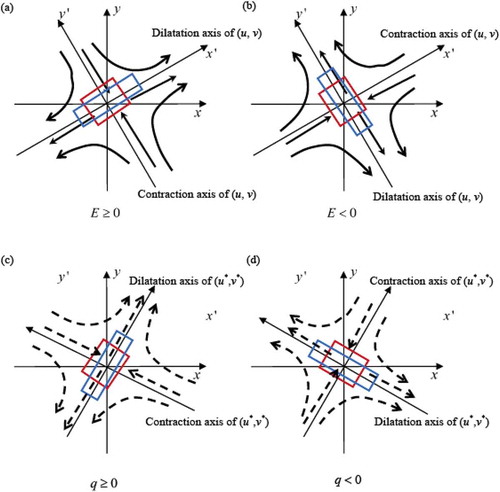
Figure 1. The effects of (a, b) deformation and (c, d) potential deformation on a fluid element. Thick black arrows in (a, b) are wind fields $\left(u,v\right)$, while dotted black arrows in (c, d) are thermodynamic-weighted velocities $\left(u^{\ast },v^{\ast }\right)$. The red square is the fluid element at the origin, while the blue square is the original element after the effects of deformation or potential deformation. In (a, c), deformation and potential deformation have positive values and they act to stretch the fluid element along the $x^{\prime }$ axis, which is called the dilatation axis, and compress it along the $y^{\prime }$ axis, which is called contraction axis. In (b, d), deformation and potential deformation have negative values and they act to stretch the fluid element along the $y^{\prime }$ axis (also the dilatation axis), and compress it along the $x^{\prime }$ axis (also the contraction axis). The illustrations of deformation in (a, b) are from Bluestein (1992). To find whether q is positive or negative, one can use Equation (13)(13) $q_{\mathrm{s}\mathrm{t}}=-\frac{\mathrm{\partial }u}{\mathrm{\partial }p}\frac{\mathrm{\partial }{\theta }^{\ast }}{\mathrm{\partial }x}+\frac{\mathrm{\partial }v}{\mathrm{\partial }p}\frac{\mathrm{\partial }{\theta }^{\ast }}{\mathrm{\partial }y}+E_{\mathrm{s}\mathrm{t}}^{\hspace{0.17em}}\frac{\mathrm{\partial }{\theta }^{\ast }}{\mathrm{\partial }p}=\frac{\mathrm{\partial }{u}^{\ast }}{\mathrm{\partial }x}-\frac{\mathrm{\partial }{v}^{\ast }}{\mathrm{\partial }y}$(13) . Equation (14)(14) $q_{\mathrm{s}\mathrm{h}}=-\frac{\mathrm{\partial }v}{\mathrm{\partial }p}\frac{\mathrm{\partial }{\theta }^{\ast }}{\mathrm{\partial }x}-\frac{\mathrm{\partial }u}{\mathrm{\partial }p}\frac{\mathrm{\partial }{\theta }^{\ast }}{\mathrm{\partial }y}+E_{\mathrm{s}\mathrm{h}}^{\hspace{0.17em}}\frac{\mathrm{\partial }{\theta }^{\ast }}{\mathrm{\partial }p}=\frac{\mathrm{\partial }{v}^{\ast }}{\mathrm{\partial }x}+\frac{\mathrm{\partial }{u}^{\ast }}{\mathrm{\partial }y}.$(14) gives the orientation of the dilatation axis, which describes the direction potential deformation is acting.

Taking $\frac{\mathrm{\partial }}{\mathrm{\partial }x}$(13) $+\frac{\mathrm{\partial }}{\mathrm{\partial }y}$(14) and $\frac{\mathrm{\partial }}{\mathrm{\partial }x}$(14) $-\frac{\mathrm{\partial }}{\mathrm{\partial }y}$(13), it can be derived that $u^{\ast }$ and $v^{\ast }$ satisfy

(15) $\frac{\mathrm{\partial }{q}_{\mathrm{s}\mathrm{t}}}{\mathrm{\partial }x}+\frac{\mathrm{\partial }{q}_{\mathrm{s}\mathrm{h}}}{\mathrm{\partial }y}={\text{bnabla}}^2{u}^{\ast }$(15)

and

(16) $\frac{\mathrm{\partial }{q}_{\mathrm{s}\mathrm{h}}}{\mathrm{\partial }x}-\frac{\mathrm{\partial }{q}_{\mathrm{s}\mathrm{t}}}{\mathrm{\partial }y}={\text{bnabla}}^2{v}^{\ast },$(16)

where ${\mathrm{\nabla }}^2=\frac{{\mathrm{\partial }}^2}{\mathrm{\partial }{x}^2}+\frac{{\mathrm{\partial }}^2}{\mathrm{\partial }{y}^2}$ is the two-dimensional Laplacian operator. Therefore, $u^{\ast }$ and $v^{\ast }$ may be obtained by numerically solving the above two Poisson equations with proper boundary conditions. In addition, as both $q_{\mathrm{s}\mathrm{t}}$ and $q_{\mathrm{s}\mathrm{h}}$ on the left-hand side of Equations (15)(15) $\frac{\mathrm{\partial }{q}_{\mathrm{s}\mathrm{t}}}{\mathrm{\partial }x}+\frac{\mathrm{\partial }{q}_{\mathrm{s}\mathrm{h}}}{\mathrm{\partial }y}={\text{bnabla}}^2{u}^{\ast }$(15) and (16(16) $\frac{\mathrm{\partial }{q}_{\mathrm{s}\mathrm{h}}}{\mathrm{\partial }x}-\frac{\mathrm{\partial }{q}_{\mathrm{s}\mathrm{t}}}{\mathrm{\partial }y}={\text{bnabla}}^2{v}^{\ast },$(16) ) synthetically contain dynamic $\left(u,v\right)$ and thermodynamic ${\theta }^{\ast }$ fields (Equations (2)(2) $q_{\mathrm{s}\mathrm{t}}^{\hspace{0.17em}}=-\frac{\mathrm{\partial }u}{\mathrm{\partial }p}\frac{\mathrm{\partial }{\theta }^{\ast }}{\mathrm{\partial }x}+\frac{\mathrm{\partial }v}{\mathrm{\partial }p}\frac{\mathrm{\partial }{\theta }^{\ast }}{\mathrm{\partial }y}+E_{\mathrm{s}\mathrm{t}}^{\hspace{0.17em}}\frac{\mathrm{\partial }{\theta }^{\ast }}{\mathrm{\partial }p},$(2) and (3(3) $q_{\mathrm{s}\mathrm{h}}^{\hspace{0.17em}}=-\frac{\mathrm{\partial }v}{\mathrm{\partial }p}\frac{\mathrm{\partial }{\theta }^{\ast }}{\mathrm{\partial }x}-\frac{\mathrm{\partial }u}{\mathrm{\partial }p}\frac{\mathrm{\partial }{\theta }^{\ast }}{\mathrm{\partial }y}+E_{\mathrm{s}\mathrm{h}}^{\hspace{0.17em}}\frac{\mathrm{\partial }{\theta }^{\ast }}{\mathrm{\partial }p}.$(3) )), it can be inferred that $\left(u^{\ast },v^{\ast }\right)$ is a combination of $\left(u,v\right)$ and ${\theta }^{\ast }$. Thus, for the moment, here we see them as a certain type of velocity that contains the influence of thermodynamic factors and term them thermodynamic-coupled velocities. PD reflects the confluence and diffluence of the thermodynamic-coupled velocities. As indicated in the introduction, deformation ($E^2=E_{\mathrm{s}\mathrm{h}}^2+E_{\mathrm{s}\mathrm{t}}^2$; Equations (4)(4) $E_{\mathrm{s}\mathrm{t}}^{\hspace{0.17em}}=\frac{\mathrm{\partial }u}{\mathrm{\partial }x}-\frac{\mathrm{\partial }v}{\mathrm{\partial }y}$(4) and (5(5) $E_{\mathrm{s}\mathrm{h}}^{\hspace{0.17em}}=\frac{\mathrm{\partial }v}{\mathrm{\partial }x}+\frac{\mathrm{\partial }u}{\mathrm{\partial }y}$(5) )) is a pure dynamic quantity, which greatly limits its application to precipitation diagnosis despite the evidence of a close relationship between deformation and precipitation. PD has similar characteristics to deformation, as stated above, but it couples both dynamic and thermodynamic factors, which is thus more applicable for diagnosing precipitation.

2.2 Tendency equation of PD

In Li et al. (2017), PD is written in its squared forms as

(17) $\begin{array}{rl}& q^2={\left(\frac{\mathrm{\partial }{\mathit{V}}_{\mathrm{h}}}{\mathrm{\partial }z}\right)}^2{\text{bnabla}}_{\mathrm{h}}^2{\theta }_{\hspace{0.17em}}^{\ast }+E^2{\left(\frac{\mathrm{\partial }{\theta }_{\hspace{0.17em}}^{\ast }}{\mathrm{\partial }z}\right)}^2\\ & +\left[2\left(-\frac{\mathrm{\partial }v}{\mathrm{\partial }z}\frac{\mathrm{\partial }{\theta }_{\hspace{0.17em}}^{\ast }}{\mathrm{\partial }x}-\frac{\mathrm{\partial }u}{\mathrm{\partial }z}\frac{\mathrm{\partial }{\theta }_{\hspace{0.17em}}^{\ast }}{\mathrm{\partial }y}\right)E_{\mathrm{s}\mathrm{h}}\frac{\mathrm{\partial }{\theta }_{\hspace{0.17em}}^{\ast }}{\mathrm{\partial }z}\right.\\ & +\left.2\left(-\frac{\mathrm{\partial }u}{\mathrm{\partial }z}\frac{\mathrm{\partial }{\theta }_{\hspace{0.17em}}^{\ast }}{\mathrm{\partial }x}+\frac{\mathrm{\partial }v}{\mathrm{\partial }z}\frac{\mathrm{\partial }{\theta }_{\hspace{0.17em}}^{\ast }}{\mathrm{\partial }y}\right)E_{\mathrm{s}\mathrm{t}}\frac{\mathrm{\partial }{\theta }_{\hspace{0.17em}}^{\ast }}{\mathrm{\partial }z}\right],\end{array}$(17)

where ${\mathit{V}}_{\mathrm{h}}=\left(u,v\right)$ is horizontal wind vector. Equation (17)(17) $\begin{array}{rl}& q^2={\left(\frac{\mathrm{\partial }{\mathit{V}}_{\mathrm{h}}}{\mathrm{\partial }z}\right)}^2{\text{bnabla}}_{\mathrm{h}}^2{\theta }_{\hspace{0.17em}}^{\ast }+E^2{\left(\frac{\mathrm{\partial }{\theta }_{\hspace{0.17em}}^{\ast }}{\mathrm{\partial }z}\right)}^2\\ & +\left[2\left(-\frac{\mathrm{\partial }v}{\mathrm{\partial }z}\frac{\mathrm{\partial }{\theta }_{\hspace{0.17em}}^{\ast }}{\mathrm{\partial }x}-\frac{\mathrm{\partial }u}{\mathrm{\partial }z}\frac{\mathrm{\partial }{\theta }_{\hspace{0.17em}}^{\ast }}{\mathrm{\partial }y}\right)E_{\mathrm{s}\mathrm{h}}\frac{\mathrm{\partial }{\theta }_{\hspace{0.17em}}^{\ast }}{\mathrm{\partial }z}\right.\\ & +\left.2\left(-\frac{\mathrm{\partial }u}{\mathrm{\partial }z}\frac{\mathrm{\partial }{\theta }_{\hspace{0.17em}}^{\ast }}{\mathrm{\partial }x}+\frac{\mathrm{\partial }v}{\mathrm{\partial }z}\frac{\mathrm{\partial }{\theta }_{\hspace{0.17em}}^{\ast }}{\mathrm{\partial }y}\right)E_{\mathrm{s}\mathrm{t}}\frac{\mathrm{\partial }{\theta }_{\hspace{0.17em}}^{\ast }}{\mathrm{\partial }z}\right],\end{array}$(17) shows that squared potential deformation (SPD) is composed of three components: the coupling of vertical wind shear and moist baroclinity (denoted as C1); the coupling of total deformation and moist static stability (denoted as C2); and the cross-coupling of all the above elements (denoted as C3). SPD is used instead of PD because the sign of PD has little physical meaning and can make the analysis complicated. Li et al. (2017) showed that PD and SPD have very similar distribution patterns during the process of precipitation, and used SPD and its three components to find the connection between PD and MCS precipitation from the perspective of the precipitation-favorable information contained in PD. However, the physical process of how the large PD anomalies form during heavy precipitation and what role the synoptic environment described by PD has in precipitation evolution cannot be acquired from only Equation (17)(17) $\begin{array}{rl}& q^2={\left(\frac{\mathrm{\partial }{\mathit{V}}_{\mathrm{h}}}{\mathrm{\partial }z}\right)}^2{\text{bnabla}}_{\mathrm{h}}^2{\theta }_{\hspace{0.17em}}^{\ast }+E^2{\left(\frac{\mathrm{\partial }{\theta }_{\hspace{0.17em}}^{\ast }}{\mathrm{\partial }z}\right)}^2\\ & +\left[2\left(-\frac{\mathrm{\partial }v}{\mathrm{\partial }z}\frac{\mathrm{\partial }{\theta }_{\hspace{0.17em}}^{\ast }}{\mathrm{\partial }x}-\frac{\mathrm{\partial }u}{\mathrm{\partial }z}\frac{\mathrm{\partial }{\theta }_{\hspace{0.17em}}^{\ast }}{\mathrm{\partial }y}\right)E_{\mathrm{s}\mathrm{h}}\frac{\mathrm{\partial }{\theta }_{\hspace{0.17em}}^{\ast }}{\mathrm{\partial }z}\right.\\ & +\left.2\left(-\frac{\mathrm{\partial }u}{\mathrm{\partial }z}\frac{\mathrm{\partial }{\theta }_{\hspace{0.17em}}^{\ast }}{\mathrm{\partial }x}+\frac{\mathrm{\partial }v}{\mathrm{\partial }z}\frac{\mathrm{\partial }{\theta }_{\hspace{0.17em}}^{\ast }}{\mathrm{\partial }y}\right)E_{\mathrm{s}\mathrm{t}}\frac{\mathrm{\partial }{\theta }_{\hspace{0.17em}}^{\ast }}{\mathrm{\partial }z}\right],\end{array}$(17) . Therefore, we derive the tendency equation of SPD to explore the above questions.

Conducting $\frac{\mathrm{\partial }}{\mathrm{\partial }t}+\mathit{V}\cdot \text{bnabla}$ to $q_{\mathrm{s}\mathrm{t}}$ and $q_{\mathrm{s}\mathrm{h}}$ (Equations (2)(2) $q_{\mathrm{s}\mathrm{t}}^{\hspace{0.17em}}=-\frac{\mathrm{\partial }u}{\mathrm{\partial }p}\frac{\mathrm{\partial }{\theta }^{\ast }}{\mathrm{\partial }x}+\frac{\mathrm{\partial }v}{\mathrm{\partial }p}\frac{\mathrm{\partial }{\theta }^{\ast }}{\mathrm{\partial }y}+E_{\mathrm{s}\mathrm{t}}^{\hspace{0.17em}}\frac{\mathrm{\partial }{\theta }^{\ast }}{\mathrm{\partial }p},$(2) and (3(3) $q_{\mathrm{s}\mathrm{h}}^{\hspace{0.17em}}=-\frac{\mathrm{\partial }v}{\mathrm{\partial }p}\frac{\mathrm{\partial }{\theta }^{\ast }}{\mathrm{\partial }x}-\frac{\mathrm{\partial }u}{\mathrm{\partial }p}\frac{\mathrm{\partial }{\theta }^{\ast }}{\mathrm{\partial }y}+E_{\mathrm{s}\mathrm{h}}^{\hspace{0.17em}}\frac{\mathrm{\partial }{\theta }^{\ast }}{\mathrm{\partial }p}.$(3) )), respectively, and incorporating the motion and thermodynamic equations on the f-plane in p-coordinates for an inviscid, non-uniformly saturated atmosphere (Ran, Li, and Gao 2013), one can obtain

(18) $\frac{\mathrm{\partial }{q}_{\mathrm{s}\mathrm{t}}}{\mathrm{\partial }t}+\mathit{V}\cdot \text{bnabla}{q}_{\mathrm{s}\mathrm{t}}=f{q}_{\mathrm{s}\mathrm{h}}+\frac{{\mathrm{\partial }}^2\varphi }{\mathrm{\partial }x\mathrm{\partial }p}\frac{\mathrm{\partial }{\theta }^{\ast }}{\mathrm{\partial }x}-\frac{{\mathrm{\partial }}^2\varphi }{\mathrm{\partial }y\mathrm{\partial }p}\frac{\mathrm{\partial }{\theta }^{\ast }}{\mathrm{\partial }y}+\left(\frac{{\mathrm{\partial }}^2\varphi }{\mathrm{\partial }{y}^2}-\frac{{\mathrm{\partial }}^2\varphi }{\mathrm{\partial }{x}^2}\right)\frac{\mathrm{\partial }{\theta }^{\ast }}{\mathrm{\partial }p}$(18)

and

(19) $\frac{\mathrm{\partial }{q}_{\mathrm{s}\mathrm{h}}}{\mathrm{\partial }t}+\mathit{V}\cdot \text{bnabla}{q}_{\mathrm{s}\mathrm{h}}=-f{q}_{\mathrm{s}\mathrm{t}}+\frac{{\mathrm{\partial }}^2\varphi }{\mathrm{\partial }y\mathrm{\partial }p}\frac{\mathrm{\partial }\theta }{\mathrm{\partial }x}+\frac{{\mathrm{\partial }}^2\varphi }{\mathrm{\partial }x\mathrm{\partial }p}\frac{\mathrm{\partial }\theta }{\mathrm{\partial }y}-2\frac{{\mathrm{\partial }}^2\varphi }{\mathrm{\partial }y\mathrm{\partial }x}\frac{\mathrm{\partial }\theta }{\mathrm{\partial }p},$(19)

where $\mathit{V}=\left(u,v,w\right)$ is the three-dimensional velocity, $w$is vertical velocity. Using the geostrophic wind $u_{\mathrm{g}}=-\frac{1}{f}\frac{\mathrm{\partial }\varphi }{\mathrm{\partial }y}$ and $v_{\mathrm{g}}=\frac{1}{f}\frac{\mathrm{\partial }\varphi }{\mathrm{\partial }x}$ to substitute the ϕ-related parts in Equations (18)(18) $\frac{\mathrm{\partial }{q}_{\mathrm{s}\mathrm{t}}}{\mathrm{\partial }t}+\mathit{V}\cdot \text{bnabla}{q}_{\mathrm{s}\mathrm{t}}=f{q}_{\mathrm{s}\mathrm{h}}+\frac{{\mathrm{\partial }}^2\varphi }{\mathrm{\partial }x\mathrm{\partial }p}\frac{\mathrm{\partial }{\theta }^{\ast }}{\mathrm{\partial }x}-\frac{{\mathrm{\partial }}^2\varphi }{\mathrm{\partial }y\mathrm{\partial }p}\frac{\mathrm{\partial }{\theta }^{\ast }}{\mathrm{\partial }y}+\left(\frac{{\mathrm{\partial }}^2\varphi }{\mathrm{\partial }{y}^2}-\frac{{\mathrm{\partial }}^2\varphi }{\mathrm{\partial }{x}^2}\right)\frac{\mathrm{\partial }{\theta }^{\ast }}{\mathrm{\partial }p}$(18) and (19(19) $\frac{\mathrm{\partial }{q}_{\mathrm{s}\mathrm{h}}}{\mathrm{\partial }t}+\mathit{V}\cdot \text{bnabla}{q}_{\mathrm{s}\mathrm{h}}=-f{q}_{\mathrm{s}\mathrm{t}}+\frac{{\mathrm{\partial }}^2\varphi }{\mathrm{\partial }y\mathrm{\partial }p}\frac{\mathrm{\partial }\theta }{\mathrm{\partial }x}+\frac{{\mathrm{\partial }}^2\varphi }{\mathrm{\partial }x\mathrm{\partial }p}\frac{\mathrm{\partial }\theta }{\mathrm{\partial }y}-2\frac{{\mathrm{\partial }}^2\varphi }{\mathrm{\partial }y\mathrm{\partial }x}\frac{\mathrm{\partial }\theta }{\mathrm{\partial }p},$(19) ) obtains

(20) $\frac{\mathrm{\partial }{q}_{\mathrm{s}\mathrm{t}}}{\mathrm{\partial }t}+\mathit{V}\cdot \text{bnabla}{q}_{\mathrm{s}\mathrm{t}}=f{q}_{\mathrm{s}\mathrm{h}}-f{\bar{q}}_{\mathrm{s}\mathrm{h}}$(20)

and

(21) $\frac{\mathrm{\partial }{q}_{\mathrm{s}\mathrm{h}}}{\mathrm{\partial }t}+\mathit{V}\cdot \text{bnabla}{q}_{\mathrm{s}\mathrm{h}}=-f{q}_{\mathrm{s}\mathrm{t}}+f{\bar{q}}_{\mathrm{s}\mathrm{t}},$(21)

where

(22) ${\bar{q}}_{\mathrm{s}\mathrm{t}}=-\frac{\mathrm{\partial }{u}_{\mathrm{g}}}{\mathrm{\partial }p}\frac{\mathrm{\partial }{\theta }^{\ast }}{\mathrm{\partial }x}+\frac{\mathrm{\partial }{v}_{\mathrm{g}}}{\mathrm{\partial }p}\frac{\mathrm{\partial }{\theta }^{\ast }}{\mathrm{\partial }y}+\left(\frac{\mathrm{\partial }{u}_{\mathrm{g}}}{\mathrm{\partial }x}-\frac{\mathrm{\partial }{v}_{\mathrm{g}}}{\mathrm{\partial }y}\right)\frac{\mathrm{\partial }{\theta }^{\ast }}{\mathrm{\partial }p}$(22)

and

(23) ${\bar{q}}_{\mathrm{s}\mathrm{h}}=-\frac{\mathrm{\partial }{v}_{\mathrm{g}}}{\mathrm{\partial }p}\frac{\mathrm{\partial }{\theta }^{\ast }}{\mathrm{\partial }x}-\frac{\mathrm{\partial }{u}_{\mathrm{g}}}{\mathrm{\partial }p}\frac{\mathrm{\partial }{\theta }^{\ast }}{\mathrm{\partial }y}+\left(\frac{\mathrm{\partial }{v}_{\mathrm{g}}}{\mathrm{\partial }x}+\frac{\mathrm{\partial }{u}_{\mathrm{g}}}{\mathrm{\partial }y}\right)\frac{\mathrm{\partial }{\theta }^{\ast }}{\mathrm{\partial }p},$(23)

are potential stretching deformation and potential shearing deformation associated with geostrophic wind, respectively.

Then, the Lagrangian form of the SPD equation is given by

(24) $\frac{\mathrm{d}{q}^2}{\mathrm{d}t}=f\left(q_{\mathrm{s}\mathrm{h}}{\bar{q}}_{\mathrm{s}\mathrm{t}}-{\bar{q}}_{\mathrm{s}\mathrm{h}}{q}_{\mathrm{s}\mathrm{t}}\right).$(24)

The term on the right-hand side of Equation (24)(24) $\frac{\mathrm{d}{q}^2}{\mathrm{d}t}=f\left(q_{\mathrm{s}\mathrm{h}}{\bar{q}}_{\mathrm{s}\mathrm{t}}-{\bar{q}}_{\mathrm{s}\mathrm{h}}{q}_{\mathrm{s}\mathrm{t}}\right).$(24) is called ‘the generation term’, which is associated with ageostrophic wind. If the ageostrophic wind is very weak or the actual wind approaches the geostrophic wind, the generation term tends to zero. Then, SPD will be conserved for a non-uniformly saturated and frictionless atmosphere.

If we further introduce geostrophic potential deformation $\bar{q}$ to represent ${\bar{q}}_{\mathrm{s}\mathrm{t}}$ and ${\bar{q}}_{\mathrm{s}\mathrm{h}}$; namely,

(25) ${\bar{q}}^2={\bar{q}}_{\mathrm{s}\mathrm{t}}^2+{\bar{q}}_{\mathrm{s}\mathrm{h}}^2,$(25)

(26) $\bar{q}=\bar{q}{{}^{\prime }}_{\mathrm{s}\mathrm{t}}=\frac{{\bar{q}}_{\mathrm{s}\mathrm{t}}}{cos2{\gamma }_{\mathrm{b}}}=\frac{{\bar{q}}_{\mathrm{s}\mathrm{h}}}{sin2{\gamma }_{\mathrm{b}}},$(26)

and

(27) ${\gamma }_{\mathrm{b}}=\frac{1}{2}{tan}^{-1}\frac{{\bar{q}}_{sh}}{{\bar{q}}_{st}},$(27)

the generation term can then be rewritten as

(28) $f\left(q_{\mathrm{s}\mathrm{h}}{\bar{q}}_{\mathrm{s}\mathrm{t}}-{\bar{q}}_{\mathrm{s}\mathrm{h}}{q}_{\mathrm{s}\mathrm{t}}\right)=fq\bar{q}sin2\left({\gamma }_{\mathrm{a}}-{\gamma }_{\mathrm{b}}\right).$(28)

Here, ${\gamma }_{\mathrm{b}}$ is the angle that the coordinate needs to rotate to make the geostrophic potential shearing deformation disappear (like Equations (11)(11) $q=q{\prime }_{\mathrm{s}\mathrm{t}}^{\hspace{0.17em}}=\frac{q_{\mathrm{s}\mathrm{t}}}{cos2{\gamma }_{\mathrm{a}}}=\frac{q_{\mathrm{s}\mathrm{h}}}{sin2{\gamma }_{\mathrm{a}}}$(11) and (12)). Remember that $q$ and $\bar{q}$ in the above equation can be positive or negative, and ${\gamma }_{\mathrm{a}}$ or ${\gamma }_{\mathrm{b}}$ can be the orientation of the dilatation axis or contraction axis depending on the sign of $q$ and $\bar{q}$ (Figure 1). To make the problem easier, the orientation of the dilatation axes of PD and geostrophic PD is introduced as ${\gamma }_{\mathrm{d}\mathrm{a}}$ and ${\gamma }_{\mathrm{d}\mathrm{b}}$, respectively. According to Figure 1, if $q\ge 0$, ${\gamma }_{\mathrm{d}\mathrm{a}}={\gamma }_{\mathrm{a}}$, otherwise, ${\gamma }_{\mathrm{d}\mathrm{a}}={\gamma }_{\mathrm{a}}+\frac{\pi }{2}$. If $\bar{q}\ge 0$, ${\gamma }_{\mathrm{d}\mathrm{b}}={\gamma }_{\mathrm{b}}$, otherwise, ${\gamma }_{\mathrm{d}\mathrm{b}}={\gamma }_{\mathrm{b}}+\frac{\pi }{2}$. Therefore, one can derive that, whether $q$ and $\bar{q}$ are positive or negative, the generation term can be expressed as

(29) $f\left(q_{\mathrm{s}\mathrm{h}}{\bar{q}}_{\mathrm{s}\mathrm{t}}-{\bar{q}}_{\mathrm{s}\mathrm{h}}{q}_{\mathrm{s}\mathrm{t}}\right)=f\left|q\right|\left|\bar{q}\right|sin2\left({\gamma }_{\mathrm{d}\mathrm{a}}-{\gamma }_{\mathrm{d}\mathrm{b}}\right),$(29)

This means that whether SPD is produced or reduced is determined by the angle between the dilatation axes of PD and geostrophic PD. Specifically, when $({\gamma }_{\mathrm{d}\mathrm{a}}-{\gamma }_{\mathrm{d}\mathrm{b}})\in \left(0,\frac{\pi }{2}\right)$, SPD will be generated.

In the following section, SPD and its tendency equation are employed to diagnose the heavy rainfall event that occurred in North China during 19–20 July 2016. Here, the term ‘diagnose’ means using the SPD and the SPD tendency equation to detect the occurrence and evolution of precipitation and determine the possible mechanism for the production of SPD and thereby its influence on heavy precipitation.

3. Case study

3.1 SPD anomalies and heavy precipitation

The torrential rain event that occurred in North China during 19–20 July 2016 was a rare extreme heavy precipitation case in North China. During this process, precipitation at nine national stations exceeded the historical extreme value in Beijing, resulting in heavy casualties and economic losses. The National Centers for Environmental Prediction Global Forecast System analysis dataset was used for the analysis. The precipitation observations were obtained from the National Meteorological Center of the China Meteorological Administration.

Figure 2 presents the 700-hPa horizontal and vertical distributions of SPD (or PD tick marks) and precipitation at 0000 UTC and 0600 UTC 20 July. These two times were chosen since they belonged to the most rapid growth stage of precipitation in Beijing. As shown in Figure 2(a), at 0000 UTC, the 6-h accumulated precipitation center was over the areas of Hebei and Tianjin, with the maximum rainfall amount up to 109 mm per 6 h. At this time, precipitation in Beijing was below 50 mm per 6 h. SPD overlapped the precipitation area and showed strong anomalies. Outside the precipitation area, SPD values were less than 2 × 10⁻¹⁴ K² Pa⁻² s⁻², while within the precipitation area SPD values reached up to 18 × 10⁻¹⁴ K² Pa⁻² s⁻². Corresponding to the large values of SPD, PD tick marks (Figure 2(c)) within the precipitation area are much longer than those outside of the precipitation area. At 0600 UTC (Figure 2(b,d)), the contrast in SPD distributions between precipitation and non-precipitation areas is even stronger.

Figure 2. (a–d) Horizontal distributions of SPD (black lines; units: 10⁻¹⁴ K² Pa⁻² s⁻²) and PD tick marks (units: 10⁻⁸ K Pa⁻¹ s⁻¹) at 700 hPa; vertical cross sections of SPD (solid black lines; units: 10⁻¹⁴ K² Pa⁻² s⁻²; six intervals) along (e) 38.5°N and (f) 39.5°N, with 6-h accumulated precipitation superposed (green bars). The left-hand column is 0000 UTC and the right-hand column is 0600 UTC 20 July 2016. PD tick marks are like deformation tick marks (Bluestein 1992). Their orientations are parallel to the dilatation axis of PD and their lengths are magnitudes of PD. The color-shaded areas are 6-h accumulated precipitation.

Figure 2(a–d) provides strong evidence of the close connection between SPD and precipitation. However, comparing the times of 0000 UTC and 0600 UTC (Figure 2(a,c) versus 2(b,d)), the distributions of SPD are quite different. At 0000 UTC (Figure 2(a)), strong SPD anomalies are distributed sparsely, with two evident SPD centers, respectively, located in the northwest and east of the precipitation center. Around the northwest SPD center, PD tick marks (Figure 2(c)) are mostly west–east oriented (thick black line along 40°N), indicating a confluence of the thermally coupled flow $\left(u^{\ast },v^{\ast }\right)$ normal to these tick marks. In contrast, PD tick marks around the east SPD center are northeast–southwest oriented (thick black line along 118°E), indicating a confluence of $\left(u^{\ast },v^{\ast }\right)$ in the northwest–southeast direction. This means that the dynamic and thermodynamic information contained in $\left(u^{\ast },v^{\ast }\right)$ is concentrated mainly near the borders of the precipitation center, but not over the precipitation center. At 0600 UTC, SPD becomes more collective and organized with only one center, collocated with the precipitation center (Figure 2(b)). PD tick marks corresponding to this center (Figure 2(d)) are consistently southwest–northeast oriented and the lengths of the PD tick marks become much longer compared to Figure 2(c). In the meantime, precipitation evidently increases, with the maximum 6-h accumulated precipitation up to 137 mm per 6 h. This indicates a possible relationship between the concentrated and organized SPD and precipitation development.

By seeing how SPD becomes concentrated over the precipitation region, one may also know how the precipitation increases. As we can see from Figure 2(e,f), which show the vertical distributions of SPD over the Beijing precipitation center at 0000 UTC and 0600 UTC 20 July 2016, the increase in precipitation is evident and the difference in the SPD distribution between the two times is also apparent. At 0000 UTC in Figure 2(e), strong SPD anomalies are confined below 750 hPa within the precipitation region. The maximum SPD is located in the boundary layer below 900 hPa at about 116°E. At 0600 UTC in Figure 2(f), SPD anomalies exhibit a distinct upward extension. Large values of SPD can reach up to 500 hPa in the mid atmosphere with a center at about 750 hPa collocating with the precipitation peak location. However, in the boundary layer, SPD becomes much smaller compared with 0000 UTC. Thus, it may be inferred that the organized SPD corresponding to the precipitation center at 700 hPa at 0600 UTC in Figure 2(b) is associated with the upward extension of SPD.

3.2 Diagnosis of the SPD concentration process

To investigate the reason for the concentration process of SPD, Equation (24)(24) $\frac{\mathrm{d}{q}^2}{\mathrm{d}t}=f\left(q_{\mathrm{s}\mathrm{h}}{\bar{q}}_{\mathrm{s}\mathrm{t}}-{\bar{q}}_{\mathrm{s}\mathrm{h}}{q}_{\mathrm{s}\mathrm{t}}\right).$(24) , which is written as

(30) $\frac{\mathrm{\partial }{q}^2}{\mathrm{\partial }t}=-{\mathit{V}}_{\mathrm{h}}\cdot \text{bnabla}{q}^2-w\frac{\mathrm{\partial }{q}^2}{\mathrm{\partial }p}+f\left|q\right|\left|\bar{q}\right|sin2\left({\gamma }_{\mathrm{d}\mathrm{a}}-{\gamma }_{\mathrm{d}\mathrm{b}}\right),$(30)

is used. The terms on the right-hand side of Equation (30)(30) $\frac{\mathrm{\partial }{q}^2}{\mathrm{\partial }t}=-{\mathit{V}}_{\mathrm{h}}\cdot \text{bnabla}{q}^2-w\frac{\mathrm{\partial }{q}^2}{\mathrm{\partial }p}+f\left|q\right|\left|\bar{q}\right|sin2\left({\gamma }_{\mathrm{d}\mathrm{a}}-{\gamma }_{\mathrm{d}\mathrm{b}}\right),$(30) are, respectively, the horizontal advection term, the vertical advection term, and the Lagrangian generation term.

Figure 3 shows the vertical temporal evolution of the average SPD and its forcing (Equation (30)(30) $\frac{\mathrm{\partial }{q}^2}{\mathrm{\partial }t}=-{\mathit{V}}_{\mathrm{h}}\cdot \text{bnabla}{q}^2-w\frac{\mathrm{\partial }{q}^2}{\mathrm{\partial }p}+f\left|q\right|\left|\bar{q}\right|sin2\left({\gamma }_{\mathrm{d}\mathrm{a}}-{\gamma }_{\mathrm{d}\mathrm{b}}\right),$(30) ) over the Beijing center (38.5°–41.5°N, 116°–118°E). As in Figure 3(a), large values of SPD (black solid lines) are first present in the boundary layer accompanying the appearance of precipitation (long black dashed line) at 1200 UTC on 19 July, and gradually extend upward with precipitation development. They show an inclination (black arrow) with height during the development of precipitation.

Figure 3. (a) Time–height cross sections of the total forcing (units: 10⁻¹⁸ K² Pa⁻² s⁻³), (b) the horizontal advection term (units: 10⁻¹⁸ K² Pa⁻² s⁻³), (c) the vertical advection term (units: 10⁻¹⁸ K² Pa⁻² s⁻³), and (d) the Lagrangian generation term (units: 10⁻¹⁸ K² Pa⁻² s⁻³) for the local change of SPD, averaged over the Beijing rainfall center (38.5–41.5°N, 116°–118°E), with solid lines representing the averaged SPD and long dashed lines the averaged 6-h accumulated precipitation; and (e) the horizontal distribution of the generation term (units: 10⁻¹⁸ K² Pa⁻² s⁻³) and (f) the tick marks of PD and geostrophic PD (units: 10⁻⁶ K Pa⁻¹ s⁻¹) at 950 hPa at 0000 UTC 20 July, with 6-h accumulated precipitation shaded.

Corresponding to the development of precipitation and appearance of large SPD, the total forcing for the local change of SPD (shaded areas; the sum of the three terms on the right-hand side of Equation (30)(30) $\frac{\mathrm{\partial }{q}^2}{\mathrm{\partial }t}=-{\mathit{V}}_{\mathrm{h}}\cdot \text{bnabla}{q}^2-w\frac{\mathrm{\partial }{q}^2}{\mathrm{\partial }p}+f\left|q\right|\left|\bar{q}\right|sin2\left({\gamma }_{\mathrm{d}\mathrm{a}}-{\gamma }_{\mathrm{d}\mathrm{b}}\right),$(30) ) appears strong from 1200 UTC 19 July to 0600 UTC 21 July (Figure 3(a)). Over the whole event, negative values of the total forcing are mainly in the near-surface layer below 950 hPa. Above these negative values are strong positive values at 950–800 hPa. In the precipitation development stage, another positive center of the total forcing appears in the middle levels at 750–600 hPa. According to Figure 3(a–c), the two positive forcing centers of the total forcing are mainly caused by the vertical advection term, which means that the upward transport of SPD from low levels to middle levels is the main contributing mechanism to SPD anomalies in the atmosphere. This is consistent with the vertical SPD extension in Figure 2(e,f), and implies that vertical transport is the main factor contributing to the local concentration of SPD.

However, upward transport of SPD anomalies means that there should be a source for the anomalies, which is attributed to the generation term. As shown in Figure 3(d), the generation term shows a positive center in the boundary layers overlapping the strong SPD anomalies. Nearly in the same place, the horizontal advection term shows a strong negative center.

As stated in section 2.2, whether the SPD can be generated is determined by the angle between the dilatation axes of PD and geostrophic PD, which can be obtained from the relative orientations of PD and geostrophic PD tick marks. To see how the SPD is generated in the boundary layer, Figure 3(f,g) also depict the horizontal distribution of the generation term and the tick marks of PD and geostrophic PD at 950 hPa at 0000 UTC 20 July. As shown in Figure 3(e,f), overlapping with the precipitation center, the generation term presents strong positive values, denoting the production of SPD. Corresponding to these positive values, the angles between the dilation axes (tick marks in Figure 3(b)) of PD and geostrophic PD are mostly less than $\frac{\pi }{2}$.

To determine the role of SPD concentration in the precipitation increase, the three components of SPD in Equation (17)(17) $\begin{array}{rl}& q^2={\left(\frac{\mathrm{\partial }{\mathit{V}}_{\mathrm{h}}}{\mathrm{\partial }z}\right)}^2{\text{bnabla}}_{\mathrm{h}}^2{\theta }_{\hspace{0.17em}}^{\ast }+E^2{\left(\frac{\mathrm{\partial }{\theta }_{\hspace{0.17em}}^{\ast }}{\mathrm{\partial }z}\right)}^2\\ & +\left[2\left(-\frac{\mathrm{\partial }v}{\mathrm{\partial }z}\frac{\mathrm{\partial }{\theta }_{\hspace{0.17em}}^{\ast }}{\mathrm{\partial }x}-\frac{\mathrm{\partial }u}{\mathrm{\partial }z}\frac{\mathrm{\partial }{\theta }_{\hspace{0.17em}}^{\ast }}{\mathrm{\partial }y}\right)E_{\mathrm{s}\mathrm{h}}\frac{\mathrm{\partial }{\theta }_{\hspace{0.17em}}^{\ast }}{\mathrm{\partial }z}\right.\\ & +\left.2\left(-\frac{\mathrm{\partial }u}{\mathrm{\partial }z}\frac{\mathrm{\partial }{\theta }_{\hspace{0.17em}}^{\ast }}{\mathrm{\partial }x}+\frac{\mathrm{\partial }v}{\mathrm{\partial }z}\frac{\mathrm{\partial }{\theta }_{\hspace{0.17em}}^{\ast }}{\mathrm{\partial }y}\right)E_{\mathrm{s}\mathrm{t}}\frac{\mathrm{\partial }{\theta }_{\hspace{0.17em}}^{\ast }}{\mathrm{\partial }z}\right],\end{array}$(17) (also see Li et al. (2017)) are further analyzed. Figure 4 illustrates vertical cross-sections of all these components along the precipitation centers at 0000 UTC and 0600 UTC 20 July. By comparing Figure 4(a–f) and Figure 2(e–f), it can be seen that the coupling of vertical wind shear and moist baroclinity (C1) and the coupling of total deformation and moist static stability (C2) are the two components contributing to the distribution patterns of SPD anomalies within the precipitation areas. At 0000 UTC (Figure 4(a,c,e), SPD anomalies in the boundary layer are mainly caused by C2, denoting a horizontal confluence of moist static stability along the dilatation axis of deformation. At 0600 UTC (Figure 4(b,d,f), C2 in the boundary layer decreases and C1 in the mid-to-lower layers increases, resulting in a high-value center at 800–700 hPa similar to SPD in Figure 2(f). This indicates that the information on the abovementioned air concentration by the generation–transportation mechanism is contained in C1, i.e., the coupling of vertical wind shear and moist baroclinity (black dashed boxes in Figure 4).

Figure 4. Vertical cross-sections of SPD components (solid black lines; units: 10⁻¹⁴ K² Pa⁻² s⁻²; six intervals): (a, b) the coupling of vertical wind shear and moist baroclinity; (c, d) the coupling of total deformation and moist static stability; (e, f) the cross-coupling of all the above elements; (g, h) vertical wind shear (units: 10⁻⁴ m s⁻¹ pa⁻¹); (i, j) generalized potential temperature (units: K) and (k, l) omega (units: pa s⁻¹) along 38.5°N at 0000 UTC (left-hand column) and 39.5°N at 0600 UTC (right-hand column), with 6-h accumulated precipitation superposed (green bars). The black dashed boxes indicate the main area where the air is concentrated by the generation–transportation mechanism.

Vertical wind shear is an important enhancing mechanism for deep moist convection by strengthening the vertical gradients of pressure (Markowski and Richardson 2010). As in Figure 4(g,h), vertical wind shear at 0600 UTC around the precipitation center (116°E) reaches up to 21 × 10⁻⁴ m s⁻¹ pa⁻¹ (black dashed boxes) – much larger than that at 0000 UTC. Meanwhile, generalized potential temperature (GPT) is moist-adiabatically conserved (Gao, Wang, and Zhou 2004), which means airflow will move along the GPT surfaces. Therefore, an increasing moist baroclinity makes the GPT isolines steep and thus enhances the vertical motion component along these isolines. As shown in Figure 4(i,j), owing to the strong vertical gradients of GPT, the GPT surfaces are nearly horizontal in the boundary layer around the precipitation center and sparse in the mid-to-lower atmosphere at 0000 UTC (black dashed boxes). At 0600 UTC, in the mid-to-lower atmosphere, moist baroclinity increases evidently and the isolines become much steeper, implying a more vertical velocity component than that at 0000 UTC. As shown in Figure 4(k,l), the vertical velocity in the black dashed boxes associated with the concentrated SPD increase evidently from 0000 UTC to 0600 UTC.

4. Conclusion

On the basis of the close relationship between deformation and precipitation, Li et al. (2017) introduced a new diagnostic parameter, PD (potential deformation), for a more flexible application of deformation in the diagnosis of heavy precipitation. In this study, the physical meaning of PD, the development process of SPD during precipitation diagnosed from the PD tendency equation, and the role of SPD development in increasing precipitation are investigated. These aspects were not considered in Li et al. (2017).

It is shown that PD shares similar features to deformation but contains much more precipitation-favorable physical elements than deformation. PD is invariant relative to rotating coordinates and can be understood as a certain type of deformation of thermodynamic-coupled velocities$\left(u^{\ast },v^{\ast }\right)$. The meaning of PD to the thermodynamic-coupled velocities is like that of deformation to the wind velocities. By diagnosing PD, areas with strong confluence or diffluence of the thermodynamic-coupled velocities can be detected, and these areas are considered to be more favorable for precipitation occurrence. Then, SPD (squared potential deformation) is used for the diagnosis of a heavy rainfall event that occurred in North China on 20 July 2016. The results reaffirmed the close relationship between SPD development and strong precipitation evolution. A new finding is that, accompanying the rapid enhancement of precipitation intensity, the SPD distribution becomes more organized and concentrated. To study the reason causing the SPD’s concentration, the SPD tendency equation is derived. It is found that whether SPD is generated or reduced in the atmosphere is associated with the angle between the dilatation axes of PD and geostrophic PD. When the angle is less than $\frac{\pi }{2}$, SPD is generated. Calculation of the SPD equation indicates that the abovementioned concentrated SPD in the mid-to-lower atmosphere is associated with a generation of SPD in the boundary layer and then an upward transport of the SPD. Further diagnosis of the SPD compositions shows that the concentration of SPD is mainly related to vertical wind shear and moist baroclinity. Both of these factors can enhance vertical motions, which then cause precipitation to increase.

In this paper, the parameter PD is reaffirmed to be a good indicator of heavy precipitation. However, what should be noted is that precipitation is associated with very complicated physical and microphysical processes. PD performs well in mesoscale convection, such as the case shown in this paper, but this might not be the case for stratiform precipitation or isolated convection with weak to moderate updraft. More cases should be studied for PD, which is the aim of future work.

Disclosure statement

No potential conflict of interest was reported by the authors.

Additional information

Funding

This study was supported by the Strategic Pilot Science and Technology Special Program of the Chinese Academy of Sciences [grant number XDA17010105], the National Key Research and Development Project [grant number 2018YFC1507104], the Scientific and Technological Developing Scheme of Jilin Province [grant number 20180201035SF], and the National Natural Science Foundation of China [grant numbers 41875056, 41775140, and 41575065].

References

- Bluestein, H. B. 1977. “Synoptic-scale Deformation and Tropical Cloud Bands.” Journal of the Atmospheric Sciences 34: 891–900. doi:10.1175/1520-0469(1977)034<0891:SSDATC>2.0.CO;2.
- Bluestein, H. B. 1992. Kinematics of the Wind Field. Synoptic-dynamic Meteorology in Midlatitudes: Volume I Principles of Kinematics and Dynamics, 81–109. New York: Oxford University Press.
- Deng, Q. H. 1986. “The Deformation Field in the Planetary Boundary Layer and Heavy Rainfall.” Journal of Academy of Meteorological Science 1: 165–174 (in Chinese).
- Gao, S. T., S. Yang, M. Xue, and C. G. Cui. 2008. “Total Deformation and Its Role in Heavy Precipitation Events Associated with Deformation-dominant Flow Patterns.” Advances in Atmospheric Sciences 25 (1): 11–23. doi:10.1007/s00376-008-0011-y.
- Gao, S. T., X. R. Wang, and Y. S. Zhou. 2004. “Generation of Generalized Moist Potential Vorticity in a Frictionless and Moist Adiabatic Flow.” Geophysical Research Letters 31: L12113. doi:10.1029/2003GL019152.
- Hoskins, B. J., M. E. McIntyre, and A. W. Robertson. 1985. “On the Use and Significance of Isentropic Potential Vorticity Maps.” Quarterly Journal of the Royal Meteorological Society 111: 877–946. doi:10.1002/qj.49711147002.
- Li, N., L. K. Ran, L. N. Zhang, and S. T. Gao. 2017. “Potential Deformation and Its Application to the Diagnosis of Heavy Precipitation in Mesoscale Convective Systems.” Advances in Atmospheric Sciences 34 (7): 894–908. doi:10.1007/s00376-017-6282-4.
- Li, N., L. K. Ran, and S. T. Gao. 2016. “The Impact of Deformation Strain on a Vortex Development in a Baroclinic Moist Atmosphere.” Advances in Atmospheric Sciences 33: 233–246. doi:10.1007/s00376-015-5082-y.
- Liang, Z. M., C. G. Lu, and E. I. Tollerud. 2010. “Diagnostic Study of Generalized Moist Potential Vorticity in a Non-uniformly Saturated Atmosphere with Heavy Precipitation.” Quarterly Journal of the Royal Meteorological Society 136: 1275–1288.
- Markowski, P., and Y. Richardson. 2010. Mesoscale Meteorology in Midlatitudes, 407. Chichester: John Wiley & Sons.
- Ran, L. K., N. Li, and S. Gao. 2013. “PV-based Diagnostic Quantities of Heavy Precipitation: Solenoidal Vorticity and Potential Solenoidal Vorticity.” Journal of Geophysical Research 118: 5710–5723.
- Schubert, W. H., S. A. Hausman, M. Garcia, K. V. Ooyama, and H. C. Kuo. 2001. “Potential Vorticity in a Moist Atmosphere.” Journal of the Atmospheric Sciences 58: 3148–3157. doi:10.1175/1520-0469(2001)058<3148:PVIAMA>2.0.CO;2.