SPCTRE: sparsity-constrained fully-digital reservoir computing architecture on FPGA

Abstract

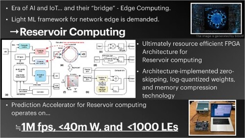
This paper proposes an unconventional architecture and algorithm for implementing reservoir computing on FPGA. An architecture-oriented algorithm with improved throughput and architecture designed to reduce memory and hardware resource requirements are presented. The proposed architecture exhibits good performance in terms of benchmarks for reservoir computing. A prediction accelerator for reservoir computing that operates on 55.45 mW at 450 K fps with <3000 LEs is realized by implementing the architecture on FPGA. The proposed approach presents a novel FPGA implementation of reservoir computing focussing on both algorithms and architecture that may serve as a basis for applications of AI at network edge.

GRAPHICAL ABSTRACT

Keywords:

• Reservoir computing
• parallel computing architecture
• FPGA implementation

1. Introduction

The integration of AI and edge computing is a challenge faced by today's information-driven society. In the context of the modern global information society, integrating artificial intelligence (AI) and edge computing remains as an important challenge in computer science. Large amounts of information including data on users' physical and environmental data can be collected easily owing to the emergence of a connected information society and the widespread implementation of Internet of things (IoT) devices. Furthermore, this information can be used to improve social services, analyse user behaviours, and improve the quality of human life. In addition, the use of artificial intelligence with such data is expected to accelerate this trend. However, existing cloud-based AI systems implemented using general-purpose hardware require a substantial amount of power and computational resources, and tend to suffer from various other problems such as privacy risks. Given this context, the demand for edge AI devices that can improve resource efficiency using hardware with limited resources specialized for ML processing is increasing [1, 2]. To this end, reservoir computing has attracted attention owing to its simple algorithms and low requirements for computational resources [3]. In this study, we propose an unconventional FPGA architecture together with an algorithm for reservoir computing that achieves high throughput with limited hardware resource requirements and high energy efficiency.

The remainder of this study is organized as follows. In Section 2, we explain the algorithms of reservoir computing and briefly introduce some related studies. In Section 3, we present the algorithms used in the proposed approach. In Section 4, we build on these concepts to describe the proposed FPGA architecture. In Section 5, we provide the results of an experimental evaluation of the proposed architecture operating on conventional benchmarks for reservoir computing. Finally, we conclude by summarizing our findings in Section 6. In addition, in Appendix 1, we discuss the proposed methods in terms of their architecture, as an appendix. We show the experimental results in terms of power consumption and resource utilization mapped on the actual FPGA.

2. Backgrounds

In this Section, we describe the backgrounds, motivation of this work and related works.

2.1. Reservoir computing

Reservoir computing is one of the recurrent neural network (RNN) frameworks known for its low computational resource requirements. The model of reservoir computing comprises an fixed-structural neural network and a separated learning system. The neural network part is called reservoir layer, and the learning system is called readout layer. The reservoir projects an input series onto a high-dimensional state space and make complex supervisors linearly separable. Unlike conventional RNN frameworks, the reservoir connections are not updated during training. The readout layer is trained to fit the supervisor by tuning the output weights. Learning is done by linear regression or gradient-based learning algorithms [4], which is much heavier than prediction algorithm in terms of computational resources. In this study, we focus on implementing reservoir computing with one-dimensional input, one-dimensional prediction, and no output feedback mechanism as a primitive model that is shown in Figure 1. The characteristics are defined as follows (Vectors are in bold small-case characters, and the matrices are in bold large characters): (1) $\begin{array}{rl}\mathbf{x}\left(t\right)& =f\left(\mathbf{Wx}\right(t-1)+{\mathbf{w}}_{\mathrm{in}}\times u(t)+\mathbf{b})\end{array}$(1) (2) $\begin{array}{rl}z\left(t\right)& ={\mathbf{w}}_{\mathrm{out}}\cdot \mathbf{x}\left(t\right)\end{array}$(2) where the terms N, $\mathbf{W}$, ${\mathbf{w}}_{\mathbf{in}}$, $\mathbf{b}$,${\mathbf{w}}_{\mathbf{out}}$, t, $\mathbf{x}\left(t\right)$, $f\left(x\right)$, $z\left(t\right)$, and $u\left(t\right)$ represent the number of network nodes, the network weight (N,N) matrix, the input weight (N,1) vector, the bias (N,1) vector, the output weight (N,1)-sized vector (trained and updated), the discrete unit of time, the state (N,1) vector of the reservoir per unit time t, the activation function (a hyperbolic tangent or identity function is often employed), the output scalar in unit time t, and the input scalar in unit time t, respectively. The following are known from reservoir computing studies:

1. The Spectral radius (explained in Section 3.2.3) of the network weight matrix must be smaller than 1, but should be close to 1 [5].

2. A network weight matrix can be a sparse matrix; its density is often smaller than 10%.

3. Each element of the network weight matrix and input weight vector is often generated as a random number.

4. However, nonzero values do not need to be distributed randomly. One such example is a cyclic reservoir [6].

   Figure 1. Basic model of reservoir computing. It has 1-D input, N-D output, and 1-D prediction. $y\left(t\right)$ is the supervisor.

   

2.2. Motivation

Reservoir computing offers a feature preferred for edge AI implementation, that is, its algorithm simplicity. Several previous studies focussed on the edge implementation of reservoir computing. Although these methods share the same objectives, their approaches vary. One possible way is a physical implementation. Many studies proposed implementing a reservoir with physical systems; for example, optical systems, chemical reactions, and analog circuits [7–10]. However, there are some challenges specific to the physical system: the resolution of the Analog to Digital / Digital to Analog conversion, and noise tolerance [11]. Many studies challenged FPGA implementation of reservoir computing with few hardware resources and high throughput, and resource efficiency was achieved by adopting mathematical approaches. Ref. [12] implements stochastic computing for reservoir computing, which helps achieve high hardware resource efficiency but lower system throughput. Architectural approaches were also reported. Ref. [13] showed that employing a bit serial adder and multiply-accumulate operation can reduce considerable hardware resources for the weight matrix, and the digital signal processors (DSPs) for multiplying. Nevertheless, the system loses throughput. These approaches are familier in the context of conventional RNN accelerators, and not specialized for the framework of Reservoir Computing.

Based on this background, we investigate an algorithm and architecture for FPGA implementation of reservoir computing that improves the resource efficiency and throughput of the system without losing accuracy. The main contributions of this work are summarized below;

• Architecture-oriented reservoir structure; Multiplexed Cyclic Reservoir, its parallel computation flow, and its FPGA architecture.

• Log-quantized internal weights; eliminate DSPs for the network calculation.

• Weight generator; eliminates random access memory(RAM) for storing weights.

• Performance enhancement of the reservoir by the spectral radius tuning method for our proposed architecture.

This study is a completed version of our previous work and includes a more detailed description and additional evaluations [14].

3. Algorithm

We propose a parallel-computation-oriented network structure: namely, the multiplexed cyclic reservoir. We further introduce the memory and computational resource reduction using a weight generator and log-quantized weights. An arbitrary application task can be processed efficiently on the later-mentioned architecture, by re-training it; adopting these algorithms.

3.1. Multiplexed cyclic reservoir

3.1.1. Concept

The network weight matrix of the reservoir is sparse, and therefore, the product of the state vector and network weight matrix involves many unnecessary calculations. This implies that the system can skip unnecessary calculations for improving throughput, i.e. zero skipping [15]. However, if the sparse areas are randomly distributed, implementing zero skipping requires complex logic such as a conditional branching mechanism. Nonetheless, Ref. [6] showed that geometric (non-randomly distribution) sparsity does not degrade the reservoir performance. If the sparse area is geometrically and regularly distributed, zero skipping can be implemented using simple combinational logic. Consequently, we design a network weight matrix with a geometric pattern-sparse area, which we refer to as a multiplexed cyclic reservoir. The network structure and matrix of the multiplexed cyclic reservoir are shown in Figure 2. Each node of the multiplexed cyclic reservoir has more than one connection to its neighbouring nodes, and as the sparsity map of Figure 2 shows, the dense area is distributed diagonally. By applying the multiplexed cyclic reservoir concept, we can adjust the density of the model, and the number of connections in each node which is defined as M. Our proposal is superior to the existing cyclic reservoir works in terms of flexibility to changes in the parameters of model. This geometrically patterned sparse matrix enables the implementation of zero skipping using simple combinational logic, and it reduces the number of multiplication and addition operations.

Figure 2. Concept of multiplexed cyclic reservoir. Geometric sparsity enables the system to implement zero skipping with simple combinational logic, and the controllable density provides flexibility to changes in the parameters of model. $\mathbf{W}$ is network weight matrix and $\mathbf{x}\left(t\right)$ is state vector.

3.1.2. Parallel computation flow

A multiplexed cyclic reservoir is compatible with a parallel processing. Upon a hardware implementations of machine learning, the reusability of data, and degree of parallelism must be addressed [16, 17]. We design a parallel computation flow paying attention to these concepts. The multiplexed cyclic reservoir only needs to use network weights that have valid values, i.e. nonzero, to calculate the state vector $\mathbf{x}\left(t\right)$, as shown in Figure 3(a). Therefore, the elements of the reservoir's state vector can be expressed using M = 2 and N = 8 as examples. (3) $\mathbf{x}\left(t\right)=\left[\begin{array}{c}f\left(x_{\left(7\right)}\right(t-1)W_{(1,7)}+x_{\left(8\right)}(t-1)W_{(1,8)}+u(t)w_{\mathrm{in}\left(1\right)}+b)\\ f\left(x_{\left(8\right)}\right(t-1)W_{(2,8)}+\mathrm{red}{x}_{\left(1\right)}(t-1)W_{(2,1)}+u(t)w_{\mathrm{in}\left(2\right)}+b)\\ f(\mathrm{red}{x}_{\left(1\right)}(t-1)W_{(3,1)}+x_{\left(2\right)}(t-1)W_{(3,2)}+u(t)w_{\mathrm{in}\left(3\right)}+b)\\ f\left(x_{\left(2\right)}\right(t-1)W_{(4,2)}+x_{\left(3\right)}(t-1)W_{(4,3)}+u(t)w_{\mathrm{in}\left(4\right)}+b)\\ ⋮\\ f\left(x_{\left(6\right)}\right(t-1)W_{(8,6)}+x_{\left(7\right)}(t-1)W_{(8,7)}+u(t)w_{\mathrm{in}\left(8\right)}+b)\end{array}\right]$(3) We define the symbols as follows: $\mathbf{x}\left(t\right)$ represents the state vector of the reservoir at unit time t, $x_{\left(1\right)}(t-1)$ represents the row-1, column-1 element of the state vector of the reservoir at unit time t−1, $W_{(1,8)}$ represents the row-1, column-8 element of the network weight matrix, and other terms are the same as in the definition from Section 2.1. In Equation  (3(3) $\mathbf{x}\left(t\right)=\left[\begin{array}{c}f\left(x_{\left(7\right)}\right(t-1)W_{(1,7)}+x_{\left(8\right)}(t-1)W_{(1,8)}+u(t)w_{\mathrm{in}\left(1\right)}+b)\\ f\left(x_{\left(8\right)}\right(t-1)W_{(2,8)}+\mathrm{red}{x}_{\left(1\right)}(t-1)W_{(2,1)}+u(t)w_{\mathrm{in}\left(2\right)}+b)\\ f(\mathrm{red}{x}_{\left(1\right)}(t-1)W_{(3,1)}+x_{\left(2\right)}(t-1)W_{(3,2)}+u(t)w_{\mathrm{in}\left(3\right)}+b)\\ f\left(x_{\left(2\right)}\right(t-1)W_{(4,2)}+x_{\left(3\right)}(t-1)W_{(4,3)}+u(t)w_{\mathrm{in}\left(4\right)}+b)\\ ⋮\\ f\left(x_{\left(6\right)}\right(t-1)W_{(8,6)}+x_{\left(7\right)}(t-1)W_{(8,7)}+u(t)w_{\mathrm{in}\left(8\right)}+b)\end{array}\right]$(3) ), the element $x_{\left(1\right)}(t-1)$ appears twice on the right-hand side of the equation, marked in red because the number of connections per node is M = 2. We design a computational flow that processes multiplications by referring to a single element of $\mathbf{x}(t-1)$ in parallel to increase the reusability of data and the degree of parallelism, as shown in Figure 3(b). This method allows us to obtain the product of $\mathbf{W}$ and $\mathbf{x}\mathbf{(}\mathbf{t}\mathbf{-}\mathbf{1}\mathbf{)}$ within almost N clock cycles. Furthermore, this technique flow reduces the hardware resource usage by avoiding the use of a multi-output-port memory. The degree of parallelism becomes M by applying this calculation flow, and it increases if the density of $\mathbf{W}$ increases. Hence, the system reaches a theoretical maximum throughput, if M (density of model) increases.

Figure 3. (a) Visualized zero skipping method. A grey arrow mean a 0 weight. (b) Parallel processing flow – product of the network matrix and state vector. The grey area is filled with 0. The red arrows and elements correspond to the red coloured terms of Equation (3(3) $\mathbf{x}\left(t\right)=\left[\begin{array}{c}f\left(x_{\left(7\right)}\right(t-1)W_{(1,7)}+x_{\left(8\right)}(t-1)W_{(1,8)}+u(t)w_{\mathrm{in}\left(1\right)}+b)\\ f\left(x_{\left(8\right)}\right(t-1)W_{(2,8)}+\mathrm{red}{x}_{\left(1\right)}(t-1)W_{(2,1)}+u(t)w_{\mathrm{in}\left(2\right)}+b)\\ f(\mathrm{red}{x}_{\left(1\right)}(t-1)W_{(3,1)}+x_{\left(2\right)}(t-1)W_{(3,2)}+u(t)w_{\mathrm{in}\left(3\right)}+b)\\ f\left(x_{\left(2\right)}\right(t-1)W_{(4,2)}+x_{\left(3\right)}(t-1)W_{(4,3)}+u(t)w_{\mathrm{in}\left(4\right)}+b)\\ ⋮\\ f\left(x_{\left(6\right)}\right(t-1)W_{(8,6)}+x_{\left(7\right)}(t-1)W_{(8,7)}+u(t)w_{\mathrm{in}\left(8\right)}+b)\end{array}\right]$(3) ).

3.2. Technologies for the network weight matrix

3.2.1. Log-quantized internal weights

The heaviest part of the calculation process in reservoir computing is the multiplication of the network weight matrix and the reservoir state vector. This process requires $N^2$ multiplications if zero-skipping is not applied, which results in a heavy load in terms of hardware resources. We applied logarithmic quantization to each element of the network weight matrix to reduce the load on hardware resources. We can replace the multipliers with a variable-bit shifter using this method. Although a variable bit shifter requires a larger circuit than a fixed-bit shifter, it still reduces hardware resource usage compared to multipliers. The process of the proposed method is summarized as (4) $\begin{array}{rl}{W}_{\mathrm{shift}(i,j)}& =\lfloor {\log }_2|W_{(i,j)}|\rfloor \end{array}$(4) (5) $\begin{array}{rl}{W}_{\mathrm{lq}(i,j)}& =\{\begin{array}{ll}\mathrm{sign}\left(W_{(i,j)}\right)\times 2^{W_{\mathrm{shift}(i,j)}}& -p\leqq W_{\mathrm{shift}(i,j)}\leqq -1\\ 0& W_{\mathrm{shift}(i,j)}<-p\\ \mathrm{sign}\left(W_{(i,j)}\right)\times \frac{1}{2}& -1<W_{\mathrm{shift}(i,j)}\end{array}\end{array}$(5) where $W_{(i,j)}$, $W_{\mathrm{lq}(i,j)}$, and $W_{\mathrm{shift}(i,j)}$ represent the row-i, column-j element of the source (non log-quantized) network weight matrix, the log-quantized expression of $W_{(i,j)}$, and the number of shift bits (i.e. exponential part of $W_{\mathrm{lq}(i,j)}$), respectively. p defines the lower limit of the weight. In this study, we used $p=6$ as an example. This formula describes the log-quantization process for $\mathbf{W}$; however, in reality, the same process is applied to the input weight matrix ${\mathbf{w}}_{\mathrm{in}}$. The system can completely eliminate the multiplier for the network calculation by applying this method. In addition, the system can compress memory resources because it stores ${\mathbf{W}}_{\mathrm{shift}}$ (the number of shifting bits), not ${\mathbf{W}}_{\mathrm{lq}}$ (log-quantized weight).

3.2.2. Weight generator

The elements of the network weight matrix are generated as random numbers and are fixed. Some researchers have used this feature to generate a network weight matrix from a resource-efficient random number generator [18, 19]. In this study, we optimize these technologies. Once the seed and the topology of the LFSR is determined, the output of the LFSR can be known before implementation. Thus, the network weight matrix of the reservoir is perfectly fixed by determining the seed and the topology of LFSR at the beginning of a prediction. The elements of $\mathbf{W}$ and ${\mathbf{w}}_{\mathrm{in}}$ are all logarithmically quantized by applying our proposal in Section 3.2.1. Thus, we use the LFSR to generate a number of shifting bits. We employ 10-bit LFSR for weights generation, and the feedback polynomial of the LFSR is described as follows: (6) $x^{10}+x^7+1$(6) Theoretically, using the conventional method, memorizing the network weight matrix requires [Bit width of output] $\times N^2$ bits of RAM. However, this method enables a system to eliminate the RAM for weights, which makes memory resources almost negligible.

3.2.3. Spectral radius tuning

The spectral radius represents the maximum absolute value of the matrix's eigenvalues. The spectral radius of $\mathbf{W}$ is expected to be close to 1. The output of the reservoir becomes saturated if the spectral radius exceeds 1. The closer it is to one, the better the performance of the reservoir is. This phenomenon is known as the ‘Edge of chaos’ [5]. In a conventional architecture, $\mathbf{W}$ is strictly tuned to meet the requirement before implementation, and the tuned weights are stored in RAM. However, the log-quantization of each element of the network weight matrix creates difficulty to tune the spectral radius because all weights are expressed as the number of shifting bits and shifting bits can not be multiplied with fixed point numbers directly. Furthermore, tuning the weights themselves is also extremly difficult because they are generated on-the-fly, and they can not be tuned before implementation. Thus, simply applying log-quantization to the weights without spectral tuning can cause the reservoir to saturate. Therefore, we propose a method to tune the spectral radius without affecting the network weight matrix by applying a scaling factor α: (7) $\mathbf{W}=\frac{{\mathbf{W}}_{\mathbf{raw}}\alpha }{\rho \left({\mathbf{W}}_{\mathbf{raw}}\right)}$(7) In Equation  (7(7) $\mathbf{W}=\frac{{\mathbf{W}}_{\mathbf{raw}}\alpha }{\rho \left({\mathbf{W}}_{\mathbf{raw}}\right)}$(7) ), ${\mathbf{W}}_{\mathrm{raw}}$ represents the network weight matrix before tuning; it is only a set of random numbers. $\rho \left(\mathbf{A}\right)$ represents the spectral radius of the matrix $\mathbf{A}$, and α represents the scaling factor ($\alpha 1$). We define the correction factor β as (8) $\text{β}=\frac{\alpha }{\rho \left({\mathbf{W}}_{\mathbf{raw}}\right)}$(8) and by combining to Equation  (2(2) $\begin{array}{rl}z\left(t\right)& ={\mathbf{w}}_{\mathrm{out}}\cdot \mathbf{x}\left(t\right)\end{array}$(2) ) the following formula is obtained (… means ‘do not care’). (9) $\begin{array}{rl}\mathbf{x}\left(t\right)& =f\left(\frac{{\mathbf{W}}_{\mathbf{raw}}\alpha }{\rho \left({\mathbf{W}}_{\mathbf{raw}}\right)}\mathbf{x}\right(t-1)+\dots \end{array}$(9) (10) $\begin{array}{rl}& \leftrightarrow \mathbf{x}\left(t\right)=f({\mathbf{W}}_{\mathbf{raw}}\mathrm{red}\text{β}\mathbf{x}(t-1)+\dots \end{array}$(10) This suggests that the correction factor does not need to be multiplied by ${\mathbf{W}}_{\mathrm{raw}}$; it can be multiplied by $\mathbf{x}(t-1)$ instead. We can calculate the correction factor before synthesis because α is a constant and ${\mathbf{W}}_{\mathrm{raw}}$, which is generated from the LFSR in our system, is predictable. Therefore, we build a system that tunes the spectral radius by multiplying β by $\mathbf{x}(t-1)$. Based on this observation, we propose a method to tune the spectral radius by tuning the state vector of the reservoir. This method enables the system to tune the spectral radius accurately using only one multiplier. Note that the proposed system require no multipliers at all if shift-based weighting is employed for the tuning.

4. Architecture

The main architecture was completed by implementing the proposed algorithms. We describe the main architecture and its pipeline timing diagram in this Section.

4.1. Main architecture

The proposed architecture is shown in Figure 4. Figure 4(a) represents the overall architecture. The Compute Unit is a module designed for network calculations, as shown in Figure 4(b). The Compute Unit has two input ports: a regular port and a weighting port. The input from the weighting port is multiplied with an element of the network weight matrix, where the multiplication is processed by variable bit shifting. The input from the regular port is not multiplied. The output of the Compute Unit is the sum of the input from the regular port and the result of variable bit shifting. An element of the network weight was generated by the LFSR. The output of the LFSR is updated at every clock cycle. The LFSR is reset when the system starts one cycle of prediction, and this process maintains the network weight matrix (which is generated by the LFSR) fixed structure in every cycle of prediction. The Spectral Radius gate is a multiplier for spectral radius tuning, as shown in Figure 4(c). The input port of the Spectral Radius gate is connected to the output of the RAM storing the state vector. The Spectral Radius gate multiplies β with each element of the state vector. The Activation Unit computes the activation function. Although we can use any computational logic as an Activation Unit, we employ an identity function, i.e. a register, without any logic. The controller controls the reset timing of LFSR and the RAM addresses.

Figure 4. Architecture of the system and its components. In this figure, we display the system for multiplexed cyclic reservoir with N = 8 and M = 2 as an example. (a) displays the overall architecture, (b) displays the architecture of the Compute Unit, (c) shows the architecture of the Spectral Radius gate, and (d) shows the architecture of the Activation Unit. The main architecture has M+1 Compute Units. The first one is used for input weighting, and the others are used for states weighting. The number of latter ones is M. (e) shows the connection map of the model, and (f) shows the sparsity map of the model. The hatched and dotted area in (b) are optimized with our proposed algorithms (mentioned in Section 3.2 and evaluated in Section 4.1). In (e) and (f), each coloured connections and elements correspond to the colour of the components from (a). For example, red coloured connections are processed by Compute Unit 0.

The system is created by combining these components. The system has one Compute Unit for input weighting (Compute Unit IN) and M Compute Units for state weighting. M corresponds to the density of the network and it is reconfigurable. The Compute Unit IN receives the bias term and the input of the reservoir, and its output port is connected to the head Compute Unit for state weighting. The Compute Units for state weighting are connected to neighbouring Compute Units for distributing the calculation of the state vector. The Activation Unit receives the output of the tail Compute Unit and calculates the elements of the state vector. The RAM stores the state vector of the reservoir. The number of words is the same as the number of nodes N. The connection map and sparsity map are shown in Figure 4(e ,f).

4.2. Pipeline chart

The overall pipeline timing diagram is presented in Figure 5(a). First, the system processes input weights and adds a bias term. The Compute Unit IN processes the sum of the bias term and the input of the reservoir and sends them to the neighbouring Compute Unit. Other Compute Units process network calculations in M clock cycles, where the network calculations are distributed among the Compute Units. The Activation Unit requires more than one clock cycle to calculate the output depending on the implemented activation function. We call the latency of the Activation Unit the activation delay, and if the activation function is implemented as an identity function, the activation delay is one clock cycle. We visualize these processes and calculations in Figure 5(b). The proposed architecture completes one prediction cycle within N+M+(Activation Delay)+2 clock cycles. Therefore, the throughput of the proposed architecture strongly depends on M, which is the number of Compute Units (or network density). This implies that decreasing the density of the network increases throughput.

Figure 5. Pipeline chart and visualized calculation flow. (a) describes the pipeline chart of the overall architecture. Each coloured process corresponds to each component of the architecture of the overall system in Figure 4(a). (b) is the calculation flow of the red marked area from (a). Only one transaction is shown for simplicity. In this figure, we employ a multiplexed cyclic reservoir with N = 8 and M = 2 and 1 clock cycle as the activation delay.

5. Algorithm evaluation

We evaluated our proposed architecture from the perspective of an algorithm by applying some benchmarks tasks.

5.1. Models and environments

For the model, we employed N = 100 and M = 5 as typical values for the evaluation, as displayed in Figure 6. Spectral radius of generated (before tuning) network weight matrix is 0.35510. Thus, to tune the spectral radius to 0.8, we set β to $\frac{0.8}{0.35510}$ = 2.25288. For the numeric expression, the bit widths of the output, input, and internal states were fixed to 32 bit, as typical values. Our prototype model employs 32-bit fixed-point arithmetic with one sign bit and 31 mantissa bits; the expression has a range of [-1,1] because the output of the reservoir is limited to [-1, 1] in many reservoir computing studies. First, we designed the behavioral model of the proposed algorithms in Python. Subsequently, we designed the RTL model of the proposed architecture in Verilog HDL and employed the Icarus Verilog 11.0 as the simulation environment. We confirmed that the outputs of the RTL model and the behavioural model matched.

Figure 6. (a) Implemented architecture for algorithm evaluation. N = 100 and M = 5. CU means Compute Unit. (b) shows the sparsity map of the model.

5.2. Benchmark; memory capacity task

First, we performed a Memory Capacity (MC) task [20]. In the MC task, the system is trained to estimate past inputs from the present outputs of the reservoir. The MC task evaluatesthe capacity of the reservoir for a linear character. For the dataset, the input was a random number series generated by the numpy library with a length of 5000 units; the dynamic range of the series was [-1,1], as in the previous studies. The generated floating-point numbers were converted into our fixed-point expression and read by the simulator. Using this dataset, we obtained the output of the reservoir using the writememh function in Icarus Verilog. The output of the reservoir is expressed as a fixed-point expressions. For the learning conditions, we applied linear regression to the outputs of the reservoir and trained the output weights. The system uses 1000 iterations for initialization, 3000 iterations for training, and 1000 iterations for prediction. The fading memory curves are shown in Figure 7(a); the result of the MC task is 43.47.

Figure 7. (a) Result of the MC task. We calculate accumulation of MCk, and got the length of linear characteristic memory; 43.47. The system can remember the input of almost 40 unit times before. (b) Result of the NARMA10 task. A comparison plot is displayed. In the pale blue area, system operates in the training phase. In the pale red area, the system operates in the prediction phase.

5.3. Benchmark; NARMA10 task

Subsequently, we performed the NARMA10 task [21]. NARMA10 is a time series with 10 previous inputs and outputs as arguments. This task is often used to evaluate the overall performance of time-series prediction, and its accuracy is evaluated using the normalized root mean square deviation (NRMSD) of the ground truth and prediction series. A lower value indicates better performance. In the benchmark, we employed almost the same method based on the MC task. For the dataset, the input was generated from the random-number inputs used in the MC task. The input series from the MC task, whose dynamic range was [-1,1], is shrunk linearly to [0,0.5]. The reservoir output from the MC task was reused during the evaluation. Length of the input and training was the same as the MC task. A comparison plot is shown in Figure 7(b). The NRMSD between the ground truth and the prediction series was equal to 0.1323. From these benchmark results, we confirmed that the proposed architecture has echo state property and exhibits good performance in linear characteristic memory.

6. Conclusion

We devised unconventional algorithms and a new architecture for reservoir computing at the network edge. The LFSR-generated weights help lower the memory resource usage to a negligible level, and the log-quantization of weights eliminates the multipliers used in typical network calculations. In addition, we devised an algorithm optimized for the reservoir computing framework, i.e. the multiplexed cyclic reservoir, and its architecture ensures efficient parallel processing, calculation reduction, and the flexibility against changes in the models. The completed architecture exhibited good performance in algorithm evaluation. Essentially, this study entailed the development of a cutting-edge technology for FPGA implementation of reservoir computing through algorithm–architecture co-design, thus contributing to the vision of the Intelligence of Things.

Acknowledgments

The authors express their sincere gratitude to Tokyo Electron Ltd. for their valuable assistance and cooperation.

Disclosure statement

No potential conflict of interest was reported by the author(s).

Appendix: Detailed architectural discussion

As the appendix, we summarize much deeper architectural discussions (hardware resources, scalabilities, breakdowns and comparisons), for interests to FPGA architecture.

A.1. Experiment setup

For the model, we employed N = 100 and M = 5 as the subjects for the evaluation (Figure 6). The numeric expression is the same as in the previous section: fixed-point number with a dynamic range [ $-1,1$]. We defined conventional architectures without the proposed method to evaluate the effectiveness of the proposed method, as summarized in Table A1.

Table A1. Comparison between conventional models and the proposed model.

	Architectures
Proposed techniques	B	C	A (Proposal)
Weight ROM requirement	Yes	No	No
Multipliers requirement	Yes	Yes	No(bit shift)
MCR architecture	Applied	Applied	Applied

Note: ${}^{\ast }$MCR means multiplexed cyclic reservoir.

Each conventional architecture employs an alternative architecture for the Compute Unit. Architecture A represents the complete architecture; i.e. the dotted and hatched areas in Figure 4 are both included. In architecture B, variable bit shifting (hatched area) is replaced with a 32-bit multiplier, while the weight generator (dotted area) is replaced with a ROM storing the network weights. In architecture C, variable bit shifting (hatched area) is replaced with a 32-bit multiplier, but the weight generator (dotted area) is left unchanged. Other features of architecture A are not changed in architectures B and C. For the compilation environment, we employed the FPGA development suite Quartus® Prime 21.10 as the implementation environment. We employed an Intel® Cyclone® IV EP4CE115F29C7N as the target FPGA.

A.2. Basic information

Table A2 lists the compilation results of the proposed architecture (Architecture A).

Table A2. Compilation results of the proposed architecture (Architecture A).

	Parameters of model	N = 100, M = 5
About model	Cycles in one prediction	109 clock cycles
About target	FPGA	Intel® Cyclone® IV EP4CE115F29C7N
Compilation	Total LE	2203
Results	Total registers	402
	Total memory bits	4096
	Total DSP (9×9 multiplier)	8
	Thermal power of core	82.40 mW

The architecture is compact and the hardware resource usage is extremely low. The thermal power was estimated using Quartus Power Analyzer. Its throughput is as high as 450 K fps prediction in 50 MHz clk. One prediction required 109 clock cycles.

A.3. Breakdowns and scalabilities

A breakdown of hardware resources and power consumption by module is shown in Figure A1. The breakdown shows that most hardware resources are occupied by the Compute Units, and the number of Logic Elements (LEs) per one Compute Unit is 322. Half the power consumption is used by the Compute Units, and one Compute Unit operates at a 3.15 mW on average. In contrast, the RAM is not dominant in terms of power consumption. This means that the size of the network (N) does not strongly affect the power consumption. However, more hardware resources and power consumption are required with an increase in the network density (M). Detailed breakdowns are summarized in Table A3. Next, we focus on the scalability of our architecture. We set two parameters (N=100 and M=5) as the typical values. However, the parameters (size and density) of the model should be reconfigurable on the field to adapt to tasks and applications. Our proposed architecture is designed to be flexible to changes in the model. Therefore, we estimated the effects on the hardware resources, power consumption, and throughput by scaling the density and size of the model. In this study, we investigated four topics: M versus a 32 bit adder and LE, N versus block RAM words, M versus power consumption and N and M versus throughput. The results are summarized in Figure A2. This figure shows that the hardware resources and power consumption scale linearly with the density of the models. The memory resource also scales linearly with the size of the models, because memory for network weights (requiring $N^2$ words) was eliminated. The throughput was scaled inversely because the clock cycle required for one prediction scaled linearly.

Figure A1. (a) LE breakdown pie graph. (b) Power breakdown pie graph. Note: The power consumption of the I/O block is excluded.

A.4. Comparison to a conventional architecture

We proposed two methods to improve the hardware resource efficiency: the weight generator and log-quantized internal weight methods. We designed conventional architectures that exclude our proposal, architectures B and C, to confirm its effectiveness, and we compared their hardware resource usage with architecture A, which is the completed architecture. We focussed on the amount of computing resources -- LE and DSP -- and BRAM to verify its effectiveness. Comparisons with the conventional architectures are presented in Figure A3.

Figure A2. (a) M versus a 32-bit adder and LE. The number of LEs is obtained by synthesizing each model; M = 1, 5, 10, and 20. Each square corresponds to actual synthesized results. (b) N versus block RAM words. (c)M versus power consumption (estimation). If the number of Compute Units increases, the power consumption increases by 3.15 mW per one Compute Unit. The square represents the compilation results. (d)N and M versus throughput. The clock frequency is 50 MHz.

Figure A3. (a) Comparisons of number of DSPs and LEs in each architecture. (b) Comparisons of BRAM usage in each architecture.

Table A3. Detailed information of breakdowns.

	Resource types
Modules	# of LEs	# of registers	Thermal power [mW]
Controller	78	10	0.33
Compute Units	1932	252	18.92
RAM	53	47	1.77
Spectral Radius gate	85	28	3.33
Other	55	65	5.88
(I/O block)	N/A	N/A	52.17
Total	2203	402	82.40

The number of LEs increased by applying the proposed method, and the number of LEs in the completed model was twice that in the conventional model. However, the number of DSPs is reduced to 14% of the conventional model in the completed model. Because the completed architecture is equipped with a variable-bit shifting logic to eliminate every DSP in the network calculation. This change enables the system to be implemented with much hardware resource hungry system, e.g; learning system. The block RAM usage was also reduced to 14% of that of the conventional model, because the weight generator eliminated RAM for network weights. These results demonstrate the effectiveness of the proposed methods.

A.5. Hardware implementation

Finally, we show the result of power consumption test of hardware implementation of the proposed architecture, as demonstration. For the model, architecture A was employed as the subject for implementation. The input to the reservoir was a random number series with a range [ $-1$,1] generated from the 6-bit LFSR. The clock signal was provided by the evaluation board's built-in 50 MHz clock. The programmed architecture operated continuously. We employed Intel® Quartus® Prime 21.10 as the FPGA programming tool, and chose the Terasic® DE2-115 as the target hardware, which is equipped within Intel® Cyclone® IV EP4CE115F29C7N. The core voltage and current were measured using a power analyser to calculate the power consumption of the FPGA. Figure  A4 shows the experimental environment. We measured the power consumption of the FPGA while the programmed architecture was continuously operated. The results of the experiment are summarized in Table A4, and the power consumption is considerably low; it is 55.45 mW.

Figure A4. Photo of the test environment.

A.6. Comparison to other works

We provide a comparison with other studies that propose FPGA implementations of reservoir computing in Table A5. Ref. [12] proposed a smart architecture with no DSPs, although its throughput is not high because of the stochastic-computing-based algorithm. Furthermore, Ref. [22] shows good hardware resource efficiency and throughput. However, our work closes to its level in terms of throughput, and beats in power consumption running almost the same size of model. The flexibility of the network density is one of our advantages. This feature allows the system to get its parameters tuning for adapting to tasks and applications on field.

Table A4. Power measurement result.

About model	Parameters of model	N = 100, M = 5
About target	FPGA	Intel® Cyclone® IV EP4CE115F29C7N
	Hardware	Terasic ® DE2-115
Result		55.45 mW

Table A5. Comparison to other works.

Informations		This work			[12]	[23]	[22]
About model	Parameters of model	N = 100	N = 50	N = 48	N = 100	$N=50$	$N=48$
	Note	$M=5$	$M=1$	$M=1$	SC based, 16bit	M = 1(Cyclic)	M = 1,TA based
About environment	Target FPGA	Cyclone IV	Cyclone IV	Cyclone IV	Cyclone IV	Cyclone III	Cyclone IV
Results	Total LE	2203	976	958	5306	1605	≈ 3000
	Total DSP	8	8	8	0	16	0
	Throughput [fps]	450 K	900 K	940 K	760	N/A	1M
	Power [W]	55.45 m	37.07 m	36.13 m	N/A	83 m	1500 m

Notes: ${}^{\ast }$ The amount of clock cycles required for one prediction is equal to N+M+4.${}^{\ast \ast }$ We choose parameters of our work to match to other implementations.

A.7. Summary of architecture evaluation

The completed architecture demonstrates its excellent hardware resource efficiency. The number of DSPs was eight, and the number of LEs was under 3000. The proposed architecture showed linear scalabilities to changes in parameters. The system completed a single prediction within 109 clock cycles; this implies that the system achieves over 450 K fps prediction by driving the proposed architecture with a 50 MHz clk. Thus, the power consumption is advantageous, and the system operates on 55.45 mW of power. This paper presents a novel approach of FPGA implementation of reservoir computing with algorithm–architecture co-design.

References

- Take it to the edge. Nat Electron. 2019;2(1):1–1. doi: 10.1038/s41928-019-0203-8
- Wang X, Han Y, Leung VCM, et al. Edge AI. Singapore: Springer; 2020. doi: 10.1007/978-981-15-6186-3
- Nakajima K, Fischer I, editors. Reservoir computing. Singapore: Springer; 2021. doi:10.1007/978-981-13-1687-6
- Sussillo D, Abbott LF. Generating coherent patterns of activity from chaotic neural networks. Neuron. 2009, 2023/07/08;63(4):544–557. doi: 10.1016/j.neuron.2009.07.018.
- Langton CG. Computation at the edge of chaos: phase transitions and emergent computation. Phys D Nonlinear Phenom. 1990;42(1–3):12–37. doi: 10.1016/0167-2789(90)90064-V
- Rodan A, Tino P. Minimum complexity echo state network. IEEE Trans Neural Netw. 2011;22(1):131–144. doi: 10.1109/TNN.2010.2089641
- Vinckier Q, Duport F, Smerieri A, et al. High-performance photonic reservoir computer based on a coherently driven passive cavity. Optica. 2015;2(5):438–446. doi: 10.1364/OPTICA.2.000438
- Akai-Kasaya M, Takeshima Y, Kan S, et al. Performance of reservoir computing in a random network of single-walled carbon nanotubes complexed with polyoxometalate. Neuromorphic Comput Eng. 2022;2(1):014003. doi: 10.1088/2634-4386/ac4339
- Kan S, Nakajima K, Asai T, et al. Physical implementation of reservoir computing through electrochemical reaction. Adv Sci. 2022;9(6):2104076. doi: 10.1002/advs.v9.6
- Kubota H, Hasegawa T, Akai-Kasaya M, et al. Noise sensitivity of physical reservoir computing in a ring array of atomic switches. Nonlinear Theory Appl IEICE. 2022;13(2):373–378. doi: 10.1587/nolta.13.373
- Soriano MC, Ortín S, Keuninckx L, et al. Delay-based reservoir computing: noise effects in a combined analog and digital implementation. IEEE Trans Neural Netw Learn Syst. 2015;26(2):388–393. doi: 10.1109/TNNLS.2014.2311855
- Alomar ML, Canals V, Perez-Mora N, et al. Fpga-based stochastic echo state networks for time-series forecasting. Intell Neuroscience. 2016 Jan;2016. doi: 10.1155/2016/3917892.
- Lin C, Liang Y, Yi Y. Fpga-based reservoir computing with optimized reservoir node architecture. In: 2022 23rd International Symposium on Quality Electronic Design (ISQED); 2022. p. 1–6.
- Abe Y, Nishida K, Ando K, et al. Sparsity-centric reservoir computing architecture. In: KJCCS 2024; Jan. NOLTA IEICE; 2024. p. Paper ID: 62.
- Gao C, Neil D, Ceolini E, et al. Deltarnn: A power-efficient recurrent neural network accelerator. In: Proceedings of the 2018 ACM/SIGDA International Symposium on Field-Programmable Gate Arrays; New York, NY, USA. Association for Computing Machinery; 2018. p. 21–30; FPGA '18. doi: 10.1145/3174243.3174261.
- Chen YH, Emer J, Sze V. Eyeriss: a spatial architecture for energy-efficient dataflow for convolutional neural networks. SIGARCH Comput Archit News. 2016;44(3):367–379. doi: 10.1145/3007787.3001177
- Bhattacharyya SS, Deprettere EF, Leupers R, et al. Handbook of signal processing systems. Switzerland: Springer International Publishing; 2019. doi:10.1007/978-3-319-91734-4.
- Abe Y, Nishida K, Akai-Kasaya M, et al. Reservoir computing with high-order polynomial activation functions and regenerative internal weights for enhancing nonlinear capacity and hardware resource efficiency. In: NOLTA'23; Sep. 26-29; Cittadella Campus of the University, Catania, Italy. NOLTA IEICE; 2023. p. 447–450.
- Gupta S, Chakraborty S, Thakur CS. Neuromorphic time-multiplexed reservoir computing with on-the-fly weight generation for edge devices. IEEE Trans Neural Netw Learn Syst. 2022;33(6):2676–2685. doi: 10.1109/TNNLS.2021.3085165
- Jaeger H. Short term memory in echo state networks. GMD Report; 2002 01.
- Atiya A, Parlos A. New results on recurrent network training: unifying the algorithms and accelerating convergence. IEEE Trans Neural Netw. 2000;11(3):697–709. doi: 10.1109/72.846741
- Galán-Prado F, Font-Rosselló J, Rosselló JL. Tropical reservoir computing hardware. IEEE Trans Circuits Syst II Express Briefs. 2020;67(11):2712–2716.
- Alomar ML, Soriano MC, Escalona-Morán M, et al. Digital implementation of a single dynamical node reservoir computer. IEEE Trans Circuits Syst II Express Briefs. 2015;62(10):977–981.