Investigating the impact of vaccine hesitancy on an emerging infectious disease: a mathematical and numerical analysis

ABSTRACT

Throughout the last two centuries, vaccines have been helpful in mitigating numerous epidemic diseases. However, vaccine hesitancy has been identified as a substantial obstacle in healthcare management. We examined the epidemiological dynamics of an emerging infection under vaccination using an SVEIR model with differential morbidity. We mathematically analyzed the model, derived ${\mathcal{R}}_0$, and provided a complete analysis of the bifurcation at ${\mathcal{R}}_0=1$. Sensitivity analysis and numerical simulations were used to quantify the tradeoffs between vaccine efficacy and vaccine hesitancy on reducing the disease burden. Our results indicated that if the percentage of the population hesitant about taking the vaccine is 10%, then a vaccine with 94% efficacy is required to reduce the peak of infections by 40%. If 60% of the population is reluctant about being vaccinated, then even a perfect vaccine will not be able to reduce the peak of infections by 40%.

KEYWORDS:

• Emerging infections
• vaccine hesitancy
• compartmental models & ODEs
• basic reproduction number
• forward bifurcations

MATHEMATICS SUBJECT CLASSIFICATIONS:

• 92-10
• 92-08
• 92B05
• 92D30
• 37G10

1. Introduction

Vaccination against infectious diseases is considered one of the most successful achievements of public health management. The world's first vaccine was demonstrated in 1796 in the UK by Dr. Edward Jenner against smallpox [1]. Since then, vaccines have been developed and successfully used in controlling and eliminating various communicable diseases including Polio, Rubella, Measles, Mumps, and Chickenpox [2]. Some vaccines are effective at blocking infection whereas other vaccines reduce the development of disease [3]. According to the CDC, mRNA vaccines for SARS-CoV-2 could potentially reduce the risk of severe symptoms by 90% [4].

Despite the successes of vaccination, however, public reluctance to inoculation has become a considerable barrier to disease control. The WHO defines vaccine hesitancy as the reluctance or refusal to vaccinate despite the availability of vaccines [5]. This phenomenon can be particularly acute in the case of emergence of a new infection, as was observed during the COVID-19 pandemic [6]. Potential reasons for vaccine hesitancy include mistrust in the health care system, religious or cultural beliefs, concerns about vaccine safety, costs, and logistical barriers, among others [7,8]. While vaccine hesitancy could lead to decreased levels of vaccine coverage and a heightened risk of disease outbreaks, experts worldwide agree that vaccine hesitancy exhibits an increasing trend [7]. However, vaccine efficacy has proven to have had a substantial effect on disease control in the past [4,9]. Therefore, this study seeks to examine the impact of vaccine efficacy and vaccine hesitancy, as well as their interplay in the control of an emerging infectious disease.

Despite the importance of vaccination in disease control, the number of ODE-based mathematical studies that consider the impact of vaccine hesitancy is modest [6,10–15]. Using a compartmental model with ODEs, Mesa et al. examine how the refusal of measles vaccines could lead to outbreaks and higher societal costs [10]. They use data on measles in England as a case study and find that even low levels of vaccine reluctance could cause a significant societal burden.

Buonomo et al. use an extended SVEIR model of COVID-19 to explore individuals' decision making on taking vaccines [6]. They use numerical simulations to demonstrate how present and past vaccine-related information influences vaccination decisions, and in turn, the dynamics of disease spread. Leung et al. use an SIRSV model of COVID-19 to explore the impact of vaccine hesitancy on disease dynamics [11]. Analytical and numerical methods demonstrate that the inclusion of vaccine hesitance in the model avoids significant biases in the process of determining the stability condition, maximum peak infection time, and threshold behaviours of their system.

In the current study, we aim to examine the impact of vaccine hesitancy on infections and deaths due to the emergence of a novel pathogen, and we ask what vaccine efficacy would be required to overcome the brunt of vaccine hesitancy. Furthermore, we investigate whether infected individuals with mild, moderate, or severe symptoms drive the disease dynamics.

The model we developed is a modified SEIR compartmental model that includes vaccination and differential morbidity and is comprised of seven compartments: susceptible, vaccinated, exposed, infected (mild symptoms), infected (moderate symptoms), infected (severe symptoms), and recovered. Our model is unique in that we consider three infected categories (mild, moderate, and severe symptoms), modeled with different transmission coefficients and recovery rates, and we include the consideration of vaccine hesitancy. The effects of vaccine hesitancy are explored by expressing vaccine coverage as a function of vaccine hesitancy, vaccine availability, and the fraction of susceptible individuals in the community. In this study, we perform a detailed mathematical analysis and use numerical simulations to answer the following research questions:

1. How does increasing the vaccine efficacy and vaccine coverage help reduce cases and deaths due to the emerging infection?

2. What is the impact of vaccine hesitancy on infections and deaths, and what efficacy of a vaccine would be required to overcome the brunt of vaccine hesitancy?

3. Which model parameters are crucial in controlling the disease burden, and how does ${\mathcal{R}}_0$ change with variation in these parameters?

4. Which class of infected individuals (i.e. mild, moderate, or severe) contributes most to the overall infection burden?

The organization of this paper is given below. An introduction to the study along with a brief review of literature is provided in Section 1 (current section). The model development is comprehensively explained in Section 2. Section 3 delves into the mathematical analysis of the model. A detailed numerical analysis of the model is presented in Section 4. Finally, a discussion of the results is given in Section 5.

2. Model development

In this study, we use a deterministic compartmental model in order to examine the dynamics of a respiratory disease caused by an emerging infectious pathogen, in the presence of vaccination that prevents infection. The model divides the total population in a hypothetical community into seven mutually exclusive compartments based on the disease status of each individual at any time t.

1. Unvaccinated susceptible (S)

2. Vaccinated susceptible (V)

3. Exposed (E)

4. Infected with mild symptoms ($I_1$)

5. Infected with moderate symptoms ($I_2$)

6. Infected with severe symptoms ($I_3$)

7. Recovered (R)

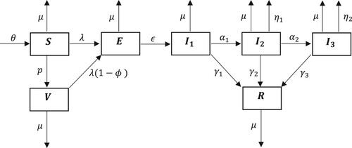
This compartmental model tracks the flow of individuals into and out of the seven states over time. The schematic diagram pertaining to the compartmental model is given in Figure 1.

Figure 1. Schematic diagram for the dynamics of an emerging disease in the presence of vaccination, with three infected classes of increasing symptom severity.

The following system of non-linear autonomous ordinary differential equations represents the inflow and outflow of individuals to and from the compartments and community over time. (1) $\begin{array}{rl}& \frac{\mathrm{d}S}{\mathrm{d}t}=\theta -(\mu +p+\lambda )S\\ & \frac{\mathrm{d}V}{\mathrm{d}t}=pS-[\mu +\lambda (1-\varphi \left)\right]V\\ & \frac{\mathrm{d}E}{\mathrm{d}t}=\lambda S+\lambda (1-\varphi )V-(\mu +ϵ)E\\ & \frac{\mathrm{d}{I}_1}{\mathrm{d}t}=ϵE-(\mu +{\alpha }_1+{\gamma }_1)I_1\\ & \frac{\mathrm{d}{I}_2}{\mathrm{d}t}={\alpha }_1{I}_1-(\mu +{\eta }_1+{\alpha }_2+{\gamma }_2)I_2\\ & \frac{\mathrm{d}{I}_3}{\mathrm{d}t}={\alpha }_2{I}_2-(\mu +{\eta }_2+{\gamma }_3)I_3\\ & \frac{\mathrm{d}R}{\mathrm{d}t}={\gamma }_1{I}_1+{\gamma }_2{I}_2+{\gamma }_3{I}_3-\mu R\end{array}$(1) The descriptions of the parameters used in the model are presented in Table 1. The parameter values used in the numerical simulations are given in Table 2.

Table 1. Definitions of parameters used in the model.

Parameter	Definition
μ	Natural mortality rate
θ	Recruitment rate
p	Vaccination coverage rate
ϕ	Vaccine efficacy
ϵ	Incubation rate
${\alpha }_1$	Rate of progression from mild symptoms to moderate symptoms
${\alpha }_2$	Rate of progression from moderate symptoms to severe symptoms
${\text{β}}_1$	Transmission coefficient for individuals infected with mild symptoms
${\text{β}}_2$	Transmission coefficient for individuals infected with moderate symptoms
${\text{β}}_3$	Transmission coefficient for individuals infected with severe symptoms
${\gamma }_1$	Recovery rate for individuals infected with mild symptoms
${\gamma }_2$	Recovery rate for individuals infected with moderate symptoms
${\gamma }_3$	Recovery rate for individuals infected with severe symptoms
${\eta }_1$	Diseased-induced death rate for individuals infected with moderate symptoms
${\eta }_2$	Diseased-induced death rate for individuals infected with severe symptoms

Table 2. Parameter values used for numerical simulations.

Parameter	Value	Units	Source/s
μ	2.7e−5	$\frac{1}{\mathrm{d}\mathrm{a}\mathrm{y}}$	Assumed *
θ	0.277	$\frac{\mathrm{i}\mathrm{n}\mathrm{d}\mathrm{i}\mathrm{v}\mathrm{i}\mathrm{d}\mathrm{u}\mathrm{a}\mathrm{l}}{\mathrm{d}\mathrm{a}\mathrm{y}}$	Set to $\mu N\left(0\right)$
p	0.05	$\frac{1}{\mathrm{d}\mathrm{a}\mathrm{y}}$	Assumed ^†
ϕ	95%	$\mathrm{d}\mathrm{i}\mathrm{m}\mathrm{e}\mathrm{n}\mathrm{s}\mathrm{i}\mathrm{o}\mathrm{n}\mathrm{l}\mathrm{e}\mathrm{s}\mathrm{s}$	[16,17]
ϵ	0.084	$\frac{1}{\mathrm{d}\mathrm{a}\mathrm{y}}$	[16,18–20]
${\alpha }_1$	0.06	$\frac{1}{\mathrm{d}\mathrm{a}\mathrm{y}}$	Assumed ^‡
${\alpha }_2$	0.01	$\frac{1}{\mathrm{d}\mathrm{a}\mathrm{y}}$	Assumed ^§
${\text{β}}_1$	4e−4	$\frac{1}{\mathrm{i}\mathrm{n}\mathrm{d}\mathrm{i}\mathrm{v}\mathrm{i}\mathrm{d}\mathrm{u}\mathrm{a}\mathrm{l}\times \mathrm{d}\mathrm{a}\mathrm{y}}$	[16,19,20]
${\text{β}}_2$	3e−4	$\frac{1}{\mathrm{i}\mathrm{n}\mathrm{d}\mathrm{i}\mathrm{v}\mathrm{i}\mathrm{d}\mathrm{u}\mathrm{a}\mathrm{l}\times \mathrm{d}\mathrm{a}\mathrm{y}}$	[16,19]
${\text{β}}_3$	2e−4	$\frac{1}{\mathrm{i}\mathrm{n}\mathrm{d}\mathrm{i}\mathrm{v}\mathrm{i}\mathrm{d}\mathrm{u}\mathrm{a}\mathrm{l}\times \mathrm{d}\mathrm{a}\mathrm{y}}$	[16,19,20]
${\gamma }_1$	0.2	$\frac{1}{\mathrm{d}\mathrm{a}\mathrm{y}}$	[16,19,20]
${\gamma }_2$	0.1	$\frac{1}{\mathrm{d}\mathrm{a}\mathrm{y}}$	[16,19]
${\gamma }_3$	0.08	$\frac{1}{\mathrm{d}\mathrm{a}\mathrm{y}}$	[16,19,20]
${\eta }_1$	0.009	$\frac{1}{\mathrm{d}\mathrm{a}\mathrm{y}}$	Assumed ^#
${\eta }_2$	0.011	$\frac{1}{\mathrm{d}\mathrm{a}\mathrm{y}}$	[16,21]

Note: Since the study is focused on an emerging respiratory infection, we use parameter values drawn from the literature of COVID-19, which is the most recent respiratory infection to affect the world at a pandemic level.*Since the population used for the simulations is hypothetical, the value for μ was chosen based upon values from the general literature.^†This value was assigned based upon a 5% vaccination coverage rate. ^{‡, §} These values were assumed based on the value of ϵ and the relation $ϵ<{\alpha }_1<{\alpha }_2$. ^# This value was assumed based on the value of ${\eta }_2$ and the relation ${\eta }_1<{\eta }_2$.

A few examples of previous models with differential morbidity in the context of COVID-19 can be found in the literature [3,20,22]. In particular, Šušteršić et al. [20] includes a classification of infected individuals on the spectrum of mild, severe, and critical symptoms. Moreover, some vaccines may only block infections, whereas others would only provide protection against severe disease, but not infection [3,23,24]. In particular, Beukenhorst et al. [3] focus on understanding which type of vaccination strategies would be more effective at a population level.

Key assumptions used in developing the model are as follows:

1. Demography. Susceptible (S) individuals are recruited at a rate θ. The natural community mortality rate due to factors excluding the disease is denoted by μ.

2. Infection. The per-capita force of infection is the sum $\lambda ={\text{β}}_1{I}_1+{\text{β}}_2{I}_3+{\text{β}}_3{I}_3$, where $I_1$ through $I_3$ are the infected compartments, and ${\text{β}}_1$ through ${\text{β}}_3$ are transmission coefficients. Transmission occurs by mass action; the per-time rate of influx to the exposed (E) compartment due to infection of susceptible individuals is $\lambda S$.

3. Leaky vaccine. The vaccine is imperfect (or leaky), with efficacy $\varphi \in [0,1]$, understood as the percentage chance that the vaccine will successfully protect an individual from infection. Susceptible individuals (S) are vaccinated at per capita vaccine coverage rate p, at which point they enter the vaccinated (V) compartment. Vaccinated individuals can become exposed (E), in the event of vaccine failure, at per-time rate $(1-\varphi )\lambda V$. A leaky vaccine with similar traits can be found in Esteban & Almodovar-Abreu [17].

4. Disease progression. Exposed individuals (E) become infected with mild symptoms ($I_1$) after an incubation period of $1/ϵ$ days. Individuals infected with mild symptoms ($I_1$) can progress to the state of moderate symptoms ($I_2$) according to the rate ${\alpha }_1$ or recover at the rate ${\gamma }_1$. Once acquiring moderate symptoms, individuals can progress to severe symptoms ($I_3$) at the rate ${\alpha }_2$, recover at the rate ${\gamma }_2$, or die due to disease at the rate ${\eta }_1$. Individuals with severe symptoms can recover at the rate ${\gamma }_3$ or die due to disease at the rate ${\eta }_2$.

5. Severity of infection. Individuals infected with mild symptoms are more likely to be in the community spreading the infection as opposed to those infected with moderate and severe symptoms, who may self-isolate or be quarantined or hospitalized. We therefore assume ${\text{β}}_1>{\text{β}}_2>{\text{β}}_3$. We also assume that more severe infections are more deadly, and therefore ${\eta }_2>{\eta }_1>\mu$. Finally, we assume that more severe infections require longer to clear, and so we assume ${\gamma }_1>{\gamma }_2>{\gamma }_3$.

6. Single viral strain. Due to the complexities of disease spread caused by the coexistence of multiple viral variants, the current model is limited to a single variant. Since we do not consider the generation of mutant variants that are most likely responsible for reinfection, we assume that recovery from the disease induces long-term immunity, which excludes the possibility of reinfections. Previous studies exclude the waning of disease-induced and/or vaccine-induced immunity for similar reasons [17,18,20,25–27].

2.1. Functional form of vaccine coverage in consideration of vaccine hesitancy

In this work, we consider the model (1(1) $\begin{array}{rl}& \frac{\mathrm{d}S}{\mathrm{d}t}=\theta -(\mu +p+\lambda )S\\ & \frac{\mathrm{d}V}{\mathrm{d}t}=pS-[\mu +\lambda (1-\varphi \left)\right]V\\ & \frac{\mathrm{d}E}{\mathrm{d}t}=\lambda S+\lambda (1-\varphi )V-(\mu +ϵ)E\\ & \frac{\mathrm{d}{I}_1}{\mathrm{d}t}=ϵE-(\mu +{\alpha }_1+{\gamma }_1)I_1\\ & \frac{\mathrm{d}{I}_2}{\mathrm{d}t}={\alpha }_1{I}_1-(\mu +{\eta }_1+{\alpha }_2+{\gamma }_2)I_2\\ & \frac{\mathrm{d}{I}_3}{\mathrm{d}t}={\alpha }_2{I}_2-(\mu +{\eta }_2+{\gamma }_3)I_3\\ & \frac{\mathrm{d}R}{\mathrm{d}t}={\gamma }_1{I}_1+{\gamma }_2{I}_2+{\gamma }_3{I}_3-\mu R\end{array}$(1) ) with two different choices for the vaccination coverage rate p. The simpler of the two is when it is treated as constant; see Section 3 for mathematical analysis and Sections 4.1 and 4.2 for numerical analysis. In the alternative, we focus on the impact of vaccine hesitancy and define a time-dependent vaccine coverage rate. We derive the functional form for the coverage rate as follows.

We assume that the per-capita vaccination rate is proportional, with proportionality (rate) constant k, to the probability that a randomly selected member of the population is both susceptible and vaccine-approving (i.e. not hesitant). Assume the probability of a randomly sampled member of the population being vaccine-hesitant is ψ, so that $1-\psi$ is the probability that the individual is vaccine-approving. The probability of a randomly sampled member of the population being susceptible is $\frac{S}{N}$, where $N=S+V+E+I_1+I_2+I_3+R$ is the total community population. Assuming these sampling events are independent, the probability of a random individual being susceptible and vaccine-approving is $(1-\psi )\frac{S}{N}$. Using the definition of the proportionality (rate) constant k, we arrive at the formula (2) $p=k(1-\psi )\frac{S}{N}.$(2) The simulations in Sections 4.3 and 4.4 are based on the functional form of p given in (2(2) $p=k(1-\psi )\frac{S}{N}.$(2) ).

3. Mathematical analysis of the model

This section is organized as follows. In Section 3.1, we present some elementary mathematical properties of the model. The disease-free equilibrium, basic reproduction number, and its threshold properties are proven in Section 3.2. In Section 3.3, we discuss the details surrounding the endemic equilibrium. The bifurcation at ${\mathcal{R}}_0=1$ is analyzed in Section 3.4.

We will frequently make use of a collection of aggregate loss rate parameters: $\begin{array}{rl}{L}_1& =\mu +{\alpha }_1+{\gamma }_1,\\ L_2& =\mu +{\eta }_1+{\alpha }_2+{\gamma }_2,\\ L_3& =\mu +{\eta }_2+{\gamma }_3,\end{array}$which represent the total loss rates from the infectious compartments $I_1,I_2$ and $I_3$, respectively. They will allow for more compact expressions in the subsequent sections.

3.1. Preliminary results

Since the model (1(1) $\begin{array}{rl}& \frac{\mathrm{d}S}{\mathrm{d}t}=\theta -(\mu +p+\lambda )S\\ & \frac{\mathrm{d}V}{\mathrm{d}t}=pS-[\mu +\lambda (1-\varphi \left)\right]V\\ & \frac{\mathrm{d}E}{\mathrm{d}t}=\lambda S+\lambda (1-\varphi )V-(\mu +ϵ)E\\ & \frac{\mathrm{d}{I}_1}{\mathrm{d}t}=ϵE-(\mu +{\alpha }_1+{\gamma }_1)I_1\\ & \frac{\mathrm{d}{I}_2}{\mathrm{d}t}={\alpha }_1{I}_1-(\mu +{\eta }_1+{\alpha }_2+{\gamma }_2)I_2\\ & \frac{\mathrm{d}{I}_3}{\mathrm{d}t}={\alpha }_2{I}_2-(\mu +{\eta }_2+{\gamma }_3)I_3\\ & \frac{\mathrm{d}R}{\mathrm{d}t}={\gamma }_1{I}_1+{\gamma }_2{I}_2+{\gamma }_3{I}_3-\mu R\end{array}$(1) ) is defined by a polynomial vector field, local existence and uniqueness of solutions are guaranteed. We will therefore only focus on non-negativity and boundedness properties.

Proposition 3.1

Non-negativity and Boundedness of Solutions

All solutions of system (1(1) $\begin{array}{rl}& \frac{\mathrm{d}S}{\mathrm{d}t}=\theta -(\mu +p+\lambda )S\\ & \frac{\mathrm{d}V}{\mathrm{d}t}=pS-[\mu +\lambda (1-\varphi \left)\right]V\\ & \frac{\mathrm{d}E}{\mathrm{d}t}=\lambda S+\lambda (1-\varphi )V-(\mu +ϵ)E\\ & \frac{\mathrm{d}{I}_1}{\mathrm{d}t}=ϵE-(\mu +{\alpha }_1+{\gamma }_1)I_1\\ & \frac{\mathrm{d}{I}_2}{\mathrm{d}t}={\alpha }_1{I}_1-(\mu +{\eta }_1+{\alpha }_2+{\gamma }_2)I_2\\ & \frac{\mathrm{d}{I}_3}{\mathrm{d}t}={\alpha }_2{I}_2-(\mu +{\eta }_2+{\gamma }_3)I_3\\ & \frac{\mathrm{d}R}{\mathrm{d}t}={\gamma }_1{I}_1+{\gamma }_2{I}_2+{\gamma }_3{I}_3-\mu R\end{array}$(1) ) with non-negative initial conditions remain bounded and non-negative for all $t\ge 0$.

Proof.

We show that no component of the model can leave the positive orthant. First, suppose that $S\left(0\right)>0$, but there exists a time $t_1$ such that $S\left(t_1\right)=0$. Let $t_1$ be minimal; that is, $t_1=inf\{t:S(t)\le 0\}$. Then $\dot{S}\left(t_1\right)\ge \theta >0$, which implies $S(t_1-s)<0$ for all s>0 sufficiently small. This contradicts the definition of $t_1$. Therefore, $S\left(t\right)>0$ for all $t\ge 0$ where it is defined. Similarly, if $S\left(0\right)=0$, then $S\left(t\right)>0$ for all t>0.

Given the above analysis, the second equation of system (1(1) $\begin{array}{rl}& \frac{\mathrm{d}S}{\mathrm{d}t}=\theta -(\mu +p+\lambda )S\\ & \frac{\mathrm{d}V}{\mathrm{d}t}=pS-[\mu +\lambda (1-\varphi \left)\right]V\\ & \frac{\mathrm{d}E}{\mathrm{d}t}=\lambda S+\lambda (1-\varphi )V-(\mu +ϵ)E\\ & \frac{\mathrm{d}{I}_1}{\mathrm{d}t}=ϵE-(\mu +{\alpha }_1+{\gamma }_1)I_1\\ & \frac{\mathrm{d}{I}_2}{\mathrm{d}t}={\alpha }_1{I}_1-(\mu +{\eta }_1+{\alpha }_2+{\gamma }_2)I_2\\ & \frac{\mathrm{d}{I}_3}{\mathrm{d}t}={\alpha }_2{I}_2-(\mu +{\eta }_2+{\gamma }_3)I_3\\ & \frac{\mathrm{d}R}{\mathrm{d}t}={\gamma }_1{I}_1+{\gamma }_2{I}_2+{\gamma }_3{I}_3-\mu R\end{array}$(1) ) leads to $\frac{\mathrm{d}V}{\mathrm{d}t}=pS-[\mu +\lambda (1-\varphi \left)\right]V\ge -[\mu +\lambda (1-\varphi \left)\right]V$as $S\left(t\right)\ge 0$ for all $t\ge 0$. Solving this differential inequality, we get $V\left(t\right)\ge V\left(0\right)\exp (-\mu t-(1-\varphi \left){\int }_0^t\right({\text{β}}_1{I}_1\left(s\right)+{\text{β}}_2{I}_2\left(s\right)+{\text{β}}_3{I}_3\left(s\right)\left)\mathrm{d}s\right)\ge 0.$Similarly, by the third equation of system (1(1) $\begin{array}{rl}& \frac{\mathrm{d}S}{\mathrm{d}t}=\theta -(\mu +p+\lambda )S\\ & \frac{\mathrm{d}V}{\mathrm{d}t}=pS-[\mu +\lambda (1-\varphi \left)\right]V\\ & \frac{\mathrm{d}E}{\mathrm{d}t}=\lambda S+\lambda (1-\varphi )V-(\mu +ϵ)E\\ & \frac{\mathrm{d}{I}_1}{\mathrm{d}t}=ϵE-(\mu +{\alpha }_1+{\gamma }_1)I_1\\ & \frac{\mathrm{d}{I}_2}{\mathrm{d}t}={\alpha }_1{I}_1-(\mu +{\eta }_1+{\alpha }_2+{\gamma }_2)I_2\\ & \frac{\mathrm{d}{I}_3}{\mathrm{d}t}={\alpha }_2{I}_2-(\mu +{\eta }_2+{\gamma }_3)I_3\\ & \frac{\mathrm{d}R}{\mathrm{d}t}={\gamma }_1{I}_1+{\gamma }_2{I}_2+{\gamma }_3{I}_3-\mu R\end{array}$(1) ), we obtain $\frac{\mathrm{d}E}{\mathrm{d}t}=\lambda S+\lambda (1-\varphi )V-(\mu +ϵ)E\ge -(\mu +ϵ)E$as $S\left(t\right),V\left(t\right)\ge 0$. Solving this differential inequality yields $E\left(t\right)\ge E\left(0\right)e^{-(\mu +ϵ)t}\ge 0$. Similar calculations show that $I_1,I_2,I_3$ and R remain non-negative for all $t\ge 0$ where they are defined.

Adding all seven equations of system (1(1) $\begin{array}{rl}& \frac{\mathrm{d}S}{\mathrm{d}t}=\theta -(\mu +p+\lambda )S\\ & \frac{\mathrm{d}V}{\mathrm{d}t}=pS-[\mu +\lambda (1-\varphi \left)\right]V\\ & \frac{\mathrm{d}E}{\mathrm{d}t}=\lambda S+\lambda (1-\varphi )V-(\mu +ϵ)E\\ & \frac{\mathrm{d}{I}_1}{\mathrm{d}t}=ϵE-(\mu +{\alpha }_1+{\gamma }_1)I_1\\ & \frac{\mathrm{d}{I}_2}{\mathrm{d}t}={\alpha }_1{I}_1-(\mu +{\eta }_1+{\alpha }_2+{\gamma }_2)I_2\\ & \frac{\mathrm{d}{I}_3}{\mathrm{d}t}={\alpha }_2{I}_2-(\mu +{\eta }_2+{\gamma }_3)I_3\\ & \frac{\mathrm{d}R}{\mathrm{d}t}={\gamma }_1{I}_1+{\gamma }_2{I}_2+{\gamma }_3{I}_3-\mu R\end{array}$(1) ) together and using the non-negative nature of each component, we obtain the inequality $\frac{\mathrm{d}N}{\mathrm{d}t}\le \theta -\mu N$. It follows that $N\left(t\right)\le max\left\{N\right(0),\theta /\mu \}$ and $\underset{t\to \mathrm{\infty }}{lim sup}N\left(t\right)=\frac{\theta }{\mu }$. Therefore, solutions to system (1(1) $\begin{array}{rl}& \frac{\mathrm{d}S}{\mathrm{d}t}=\theta -(\mu +p+\lambda )S\\ & \frac{\mathrm{d}V}{\mathrm{d}t}=pS-[\mu +\lambda (1-\varphi \left)\right]V\\ & \frac{\mathrm{d}E}{\mathrm{d}t}=\lambda S+\lambda (1-\varphi )V-(\mu +ϵ)E\\ & \frac{\mathrm{d}{I}_1}{\mathrm{d}t}=ϵE-(\mu +{\alpha }_1+{\gamma }_1)I_1\\ & \frac{\mathrm{d}{I}_2}{\mathrm{d}t}={\alpha }_1{I}_1-(\mu +{\eta }_1+{\alpha }_2+{\gamma }_2)I_2\\ & \frac{\mathrm{d}{I}_3}{\mathrm{d}t}={\alpha }_2{I}_2-(\mu +{\eta }_2+{\gamma }_3)I_3\\ & \frac{\mathrm{d}R}{\mathrm{d}t}={\gamma }_1{I}_1+{\gamma }_2{I}_2+{\gamma }_3{I}_3-\mu R\end{array}$(1) ) are bounded.

Remark: It is important to verify whether the state variables of system (1(1) $\begin{array}{rl}& \frac{\mathrm{d}S}{\mathrm{d}t}=\theta -(\mu +p+\lambda )S\\ & \frac{\mathrm{d}V}{\mathrm{d}t}=pS-[\mu +\lambda (1-\varphi \left)\right]V\\ & \frac{\mathrm{d}E}{\mathrm{d}t}=\lambda S+\lambda (1-\varphi )V-(\mu +ϵ)E\\ & \frac{\mathrm{d}{I}_1}{\mathrm{d}t}=ϵE-(\mu +{\alpha }_1+{\gamma }_1)I_1\\ & \frac{\mathrm{d}{I}_2}{\mathrm{d}t}={\alpha }_1{I}_1-(\mu +{\eta }_1+{\alpha }_2+{\gamma }_2)I_2\\ & \frac{\mathrm{d}{I}_3}{\mathrm{d}t}={\alpha }_2{I}_2-(\mu +{\eta }_2+{\gamma }_3)I_3\\ & \frac{\mathrm{d}R}{\mathrm{d}t}={\gamma }_1{I}_1+{\gamma }_2{I}_2+{\gamma }_3{I}_3-\mu R\end{array}$(1) ) remain positive and bounded for all time $t\in [0,\mathrm{\infty })$ in order for the system to be epidemiologically relevant.

Proposition 3.2

Positive Invariance

The closed set $\mathrm{\Omega }=\left\{\right(S,V,E,I_1,I_2,I_3,R)\in {\mathbb{R}}_{+}^7:0\le S+V+E+I_1+I_2+I_3+R\le \frac{\theta }{\mu }\}$ is a positively invariant region for system (1(1) $\begin{array}{rl}& \frac{\mathrm{d}S}{\mathrm{d}t}=\theta -(\mu +p+\lambda )S\\ & \frac{\mathrm{d}V}{\mathrm{d}t}=pS-[\mu +\lambda (1-\varphi \left)\right]V\\ & \frac{\mathrm{d}E}{\mathrm{d}t}=\lambda S+\lambda (1-\varphi )V-(\mu +ϵ)E\\ & \frac{\mathrm{d}{I}_1}{\mathrm{d}t}=ϵE-(\mu +{\alpha }_1+{\gamma }_1)I_1\\ & \frac{\mathrm{d}{I}_2}{\mathrm{d}t}={\alpha }_1{I}_1-(\mu +{\eta }_1+{\alpha }_2+{\gamma }_2)I_2\\ & \frac{\mathrm{d}{I}_3}{\mathrm{d}t}={\alpha }_2{I}_2-(\mu +{\eta }_2+{\gamma }_3)I_3\\ & \frac{\mathrm{d}R}{\mathrm{d}t}={\gamma }_1{I}_1+{\gamma }_2{I}_2+{\gamma }_3{I}_3-\mu R\end{array}$(1) ).

Proof.

Let $N\left(t\right)$ denote the sum of all components, and suppose $N\left(0\right)\le \frac{\theta }{\mu }$ so that the initial condition is in Ω. From the proof of Proposition 3.1, we know that $N\left(t\right)\le max\left\{N\right(0),\theta /\mu \}=\frac{\theta }{\mu }.$

3.2. Disease-free equilibrium and basic reproduction number

The disease-free equilibrium (DFE), also referred to as the infection-free equilibrium, of an epidemiological ODE system is the equilibrium solution (i.e. stationary point) where all the disease related variables are equal to 0. A routine calculation yields (3) ${\mathbb{E}}^0=(\frac{\theta }{\mu +p},\frac{p\theta }{\mu (\mu +p)},0,0,0,0,0).$(3) The basic reproduction number or basic reproductive ratio, usually denoted by ${\mathcal{R}}_0$, gives valuable insights into the dynamics of an epidemic, as it delineates if an outbreak will occur or if the disease will die out. ${\mathcal{R}}_0$ is biologically defined as the expected number of secondary infections produced by a single infectious case in an otherwise completely susceptible population [28]. Mathematically, it is a threshold quantity that determines the stability of the disease-free equilibrium [28,29]. The disease spreads (i.e. an epidemic occurs) if ${\mathcal{R}}_0>1$, and it dies out if ${\mathcal{R}}_0<1$. The following theorem proves exactly this result for the case of a small outbreak. The stability of the DFE when ${\mathcal{R}}_0=1$ is treated in Lemma 3.5.

Theorem 3.3

The basic reproduction number for model (1(1) $\begin{array}{rl}& \frac{\mathrm{d}S}{\mathrm{d}t}=\theta -(\mu +p+\lambda )S\\ & \frac{\mathrm{d}V}{\mathrm{d}t}=pS-[\mu +\lambda (1-\varphi \left)\right]V\\ & \frac{\mathrm{d}E}{\mathrm{d}t}=\lambda S+\lambda (1-\varphi )V-(\mu +ϵ)E\\ & \frac{\mathrm{d}{I}_1}{\mathrm{d}t}=ϵE-(\mu +{\alpha }_1+{\gamma }_1)I_1\\ & \frac{\mathrm{d}{I}_2}{\mathrm{d}t}={\alpha }_1{I}_1-(\mu +{\eta }_1+{\alpha }_2+{\gamma }_2)I_2\\ & \frac{\mathrm{d}{I}_3}{\mathrm{d}t}={\alpha }_2{I}_2-(\mu +{\eta }_2+{\gamma }_3)I_3\\ & \frac{\mathrm{d}R}{\mathrm{d}t}={\gamma }_1{I}_1+{\gamma }_2{I}_2+{\gamma }_3{I}_3-\mu R\end{array}$(1) ) is (4) ${\mathcal{R}}_0=\frac{\theta ϵ(\mu +(1-\varphi \left)p\right)(L_2{L}_3{\text{β}}_1+L_3{\alpha }_1{\text{β}}_2+{\alpha }_1{\alpha }_2{\text{β}}_3)}{\mu (\mu +p)(\mu +ϵ)L_1{L}_2{L}_3}.$(4) The disease-free equilibrium is locally asymptotically stable if and only if ${\mathcal{R}}_0<1$, and unstable if and only if ${\mathcal{R}}_0>1$.

Proof.

To this end, we use the next-generation matrix (NGM) method developed by Diekmann et al. as well as van den Driessche and Watmough [29,30]. First, we divide the model compartments into two main categories as uninfected, $X=(S,V,R{)}^T$, and infected, $Y=(E,I_1,I_2,I_3{)}^T$. We rewrite $\frac{\mathrm{d}Y}{\mathrm{d}t}=(\frac{\mathrm{d}E}{\mathrm{d}t},\frac{\mathrm{d}{I}_1}{\mathrm{d}t},\frac{\mathrm{d}{I}_2}{\mathrm{d}t},\frac{\mathrm{d}{I}_3}{\mathrm{d}t}{)}^T$ as $\frac{\mathrm{d}Y}{\mathrm{d}t}=\mathcal{F}-\mathcal{V}$, where $\mathcal{F}=\left[\begin{array}{c}({\text{β}}_1{I}_1+{\text{β}}_2{I}_2+{\text{β}}_3{I}_3)S+({\text{β}}_1{I}_1+{\text{β}}_2{I}_2+{\text{β}}_3{I}_3)(1-\varphi )V\\ 0\\ 0\\ 0\end{array}\right]$represents all rates from X to Y, and $\mathcal{V}=\left[\begin{array}{c}(\mu +ϵ)E\\ -ϵE+L_1{I}_1\\ -{\alpha }_1{I}_1+L_2{I}_2\\ -{\alpha }_2{I}_2+L_3{I}_3\end{array}\right]$represents all other rates.

The Jacobians of $\mathcal{F}$ and $\mathcal{V}$ evaluated at the DFE given in (3(3) ${\mathbb{E}}^0=(\frac{\theta }{\mu +p},\frac{p\theta }{\mu (\mu +p)},0,0,0,0,0).$(3) ) are $F=\left[\begin{array}{cccc}0& {\displaystyle \frac{\theta (\mu +(1-\varphi \left)p\right){\text{β}}_1}{\mu (\mu +p)}}& {\displaystyle \frac{\theta (\mu +(1-\varphi \left)p\right){\text{β}}_2}{\mu (\mu +p)}}& {\displaystyle \frac{\theta (\mu +(1-\varphi \left)p\right){\text{β}}_3}{\mu (\mu +p)}}\\ 0& 0& 0& 0\\ 0& 0& 0& 0\\ 0& 0& 0& 0\end{array}\right]$and $V=\left[\begin{array}{cccc}\mu +ϵ& 0& 0& 0\\ -ϵ& L_1& 0& 0\\ 0& -{\alpha }_1& L_2& 0\\ 0& 0& -{\alpha }_2& L_3\end{array}\right].$${\mathcal{R}}_0$ is the spectral radius of the next-generation matrix $F{V}^{-1}$, and is given by (5) ${\mathcal{R}}_0=\frac{\theta (\mu +(1-\varphi \left)p\right){\text{β}}_1ϵ}{\mu (\mu +p)(\mu +ϵ)L_1}+\frac{\theta (\mu +(1-\varphi \left)p\right){\text{β}}_2ϵ{\alpha }_1}{\mu (\mu +p)(\mu +ϵ)L_1{L}_2}+\frac{\theta (\mu +(1-\varphi \left)p\right){\text{β}}_3ϵ{\alpha }_1{\alpha }_2}{\mu (\mu +p)(\mu +ϵ)L_1{L}_2{L}_3}.$(5) Then, by simplifying further, we obtain a simple expression, which we readily find is equal to (4(4) ${\mathcal{R}}_0=\frac{\theta ϵ(\mu +(1-\varphi \left)p\right)(L_2{L}_3{\text{β}}_1+L_3{\alpha }_1{\text{β}}_2+{\alpha }_1{\alpha }_2{\text{β}}_3)}{\mu (\mu +p)(\mu +ϵ)L_1{L}_2{L}_3}.$(4) ). The stability assertions follow from Theorem 2 of [29].

Remark 3.1

The expression (5(5) ${\mathcal{R}}_0=\frac{\theta (\mu +(1-\varphi \left)p\right){\text{β}}_1ϵ}{\mu (\mu +p)(\mu +ϵ)L_1}+\frac{\theta (\mu +(1-\varphi \left)p\right){\text{β}}_2ϵ{\alpha }_1}{\mu (\mu +p)(\mu +ϵ)L_1{L}_2}+\frac{\theta (\mu +(1-\varphi \left)p\right){\text{β}}_3ϵ{\alpha }_1{\alpha }_2}{\mu (\mu +p)(\mu +ϵ)L_1{L}_2{L}_3}.$(5) ) has a succinct biological interpretation. It is the sum of rates at which individuals become exposed (not yet infectious) by individuals in each of the three infectious states, weighted by the amount of time a typical individual spends in each of these states as they progress through their infection. Specifically, the unconditional (i.e. without assuming transfers between states) average length of time an individual spends with mild symptoms ($I_1$), moderate symptoms ($I_2$), and severe symptoms ($I_3$) is $1/L_1$, $1/L_2$, and $1/L_3$, respectively. The probability of the transition $E\to I_1$ is the ratio ${\mathbb{P}}_{E\to I_1}=ϵ/(ϵ+\mu )$, so that the average time spent with mild symptoms after exposure is $\frac{ϵ}{(ϵ+\mu )L_1}$. The probability of transition from $I_1\to I_2$ is ${\mathbb{P}}_{I_1\to I_2}={\alpha }_1/L_1$. Therefore, the probability of the transition $E\to I_1\to I_2$ is ${\mathbb{P}}_{E\to I_1}{\mathbb{P}}_{I_1\to I_2}=\frac{ϵ{\alpha }_1}{(ϵ+\mu )L_1}$, so that the average amount of time spent with moderate symptoms (after exposure and mild symptoms) is $\frac{ϵ{\alpha }_1}{(ϵ+\mu )L_1{L}_2}$. Similarly, the average amount of time spent with severe symptoms is $\frac{ϵ{\alpha }_1{\alpha }_2}{(ϵ+\mu )L_1{L}_2{L}_3}.$

Remark 3.2

If ${\mathcal{R}}_0<1$, the above theorem guarantees only that a sufficiently small outbreak will die out. While numerical simulations strongly suggest that global stability of the DFE (${\mathbb{E}}^0$) follows from ${\mathcal{R}}_0<1$, we make no attempt to mathematically prove that in this work.

3.3. Endemic equilibrium

The endemic equilibrium of an epidemiological ODE system is an equilibrium solution to the system where the disease-related variable(s) are not necessarily equal to 0. For this model, an explicit expression is available for the endemic equilibrium (it can be shown to be equivalent to one of the zeroes of a second degree polynomial), but the resulting formula is not especially useful due to the introduction of several very complicated bulk parameters. We instead analyze the endemic equilibrium using a more geometric approach, which can be connected to ${\mathcal{R}}_0$.

Lemma 3.4

The model (1(1) $\begin{array}{rl}& \frac{\mathrm{d}S}{\mathrm{d}t}=\theta -(\mu +p+\lambda )S\\ & \frac{\mathrm{d}V}{\mathrm{d}t}=pS-[\mu +\lambda (1-\varphi \left)\right]V\\ & \frac{\mathrm{d}E}{\mathrm{d}t}=\lambda S+\lambda (1-\varphi )V-(\mu +ϵ)E\\ & \frac{\mathrm{d}{I}_1}{\mathrm{d}t}=ϵE-(\mu +{\alpha }_1+{\gamma }_1)I_1\\ & \frac{\mathrm{d}{I}_2}{\mathrm{d}t}={\alpha }_1{I}_1-(\mu +{\eta }_1+{\alpha }_2+{\gamma }_2)I_2\\ & \frac{\mathrm{d}{I}_3}{\mathrm{d}t}={\alpha }_2{I}_2-(\mu +{\eta }_2+{\gamma }_3)I_3\\ & \frac{\mathrm{d}R}{\mathrm{d}t}={\gamma }_1{I}_1+{\gamma }_2{I}_2+{\gamma }_3{I}_3-\mu R\end{array}$(1) ) has at most one (positive) endemic equilibrium. In particular, the endemic equilibrium exists if and only if ${\mathcal{R}}_0>1$.

Proof.

Notice that any steady state $(S,V,E,I_1,I_2,I_3,R)$ of system (1(1) $\begin{array}{rl}& \frac{\mathrm{d}S}{\mathrm{d}t}=\theta -(\mu +p+\lambda )S\\ & \frac{\mathrm{d}V}{\mathrm{d}t}=pS-[\mu +\lambda (1-\varphi \left)\right]V\\ & \frac{\mathrm{d}E}{\mathrm{d}t}=\lambda S+\lambda (1-\varphi )V-(\mu +ϵ)E\\ & \frac{\mathrm{d}{I}_1}{\mathrm{d}t}=ϵE-(\mu +{\alpha }_1+{\gamma }_1)I_1\\ & \frac{\mathrm{d}{I}_2}{\mathrm{d}t}={\alpha }_1{I}_1-(\mu +{\eta }_1+{\alpha }_2+{\gamma }_2)I_2\\ & \frac{\mathrm{d}{I}_3}{\mathrm{d}t}={\alpha }_2{I}_2-(\mu +{\eta }_2+{\gamma }_3)I_3\\ & \frac{\mathrm{d}R}{\mathrm{d}t}={\gamma }_1{I}_1+{\gamma }_2{I}_2+{\gamma }_3{I}_3-\mu R\end{array}$(1) ) must satisfy the following equations: $\begin{array}{rl}S& =\frac{\theta }{\mu +p+\lambda },V=\frac{pS}{\mu +\lambda (1-\varphi )},E=\frac{\lambda (S+(1-\varphi \left)V\right)}{\mu +ϵ},\\ I_1& =\frac{ϵ}{L_1}E,I_2=\frac{{\alpha }_1ϵ}{L_1{L}_2}E,I_3=\frac{{\alpha }_1{\alpha }_2ϵ}{L_1{L}_2{L}_3}E,R=\frac{{\gamma }_1{I}_1+{\gamma }_2{I}_2+{\gamma }_3{I}_3}{\mu }.\end{array}$Recall that $\lambda ={\text{β}}_1{I}_1+{\text{β}}_2{I}_2+{\text{β}}_3{I}_3$. Hence, we obtain $\begin{array}{rl}\lambda & ={\text{β}}_1\frac{ϵ}{L_1}E+{\text{β}}_2\frac{ϵ{\alpha }_1}{L_1{L}_2}E+{\text{β}}_3\frac{ϵ{\alpha }_1{\alpha }_2}{L_1{L}_2{L}_3}E\\ & =\mathrm{\Lambda }E\end{array}$where $\mathrm{\Lambda }={\text{β}}_1\frac{ϵ}{L_1}+{\text{β}}_2\frac{ϵ{\alpha }_1}{L_1{L}_2}+{\text{β}}_3\frac{ϵ{\alpha }_1{\alpha }_2}{L_1{L}_2{L}_3}$. Substituting this into the expression for E, we get $E=\frac{1}{\mu +ϵ}\mathrm{\Lambda }E(S+(1-\varphi \left)V\right).$Suppose $E\ne 0$, so that we eliminate the disease-free equilibrium. Canceling E on both sides and substituting in S and V, we have $\begin{array}{rl}1& =\frac{\mathrm{\Lambda }}{\mu +ϵ}(S+(1-\varphi \left)V\right)=\frac{\mathrm{\Lambda }}{\mu +ϵ}S(1+\frac{(1-\varphi )p}{\mu +\mathrm{\Lambda }(1-\varphi )E})\\ & =\frac{\mathrm{\Lambda }\theta }{\mu +ϵ}\left(\frac{1}{\mu +p+\mathrm{\Lambda }E}\right)\cdot (1+\frac{(1-\varphi )p}{\mu +\mathrm{\Lambda }(1-\varphi )E}).\end{array}$Now define $\mathcal{H}:[0,\mathrm{\infty })\mapsto \mathbb{R}$ by $\mathcal{H}\left(x\right)=\frac{\mathrm{\Lambda }\theta }{\mu +ϵ}\left(\frac{1}{\mu +p+\mathrm{\Lambda }x}\right)(1+\frac{p(1-\varphi )}{\mu +\mathrm{\Lambda }(1-\varphi )x})$. Thus, the endemic equilibria are positive solutions of the non-linear equation $\mathcal{H}\left(E\right)=1$. Clearly, the function $\mathcal{H}$ is continuous and non-negative on its domain. Moreover, we have $\begin{array}{rl}{\mathcal{H}}^{\prime }\left(x\right)& =-\frac{\mathrm{\Lambda }\theta }{\mu +ϵ}[\left(\frac{1}{\mu +p+\mathrm{\Lambda }x}\right)\left(\frac{p\mathrm{\Lambda }(1-\varphi {)}^2}{(\mu +\mathrm{\Lambda }(1-\varphi )x{)}^2}\right)\\ & +\left(\frac{\mathrm{\Lambda }}{(\mu +p+\mathrm{\Lambda }x{)}^2}\right)(1+\frac{p(1-\varphi )}{\mu +\mathrm{\Lambda }(1-\varphi )x})]<0,\end{array}$for all $x\in [0,\mathrm{\infty })$. Therefore, $\mathcal{H}$ is a strictly decreasing function on its domain. In addition, we have $\underset{x\to \mathrm{\infty }}{lim}H\left(x\right)=0$. Thus, a positive solution of the equation $\mathcal{H}\left(E\right)=1$ exists if and only if $\mathcal{H}\left(0\right)>1$. Furthermore, this solution will be unique due to the monotonicity of the function $\mathcal{H}$. Also, no endemic equilibrium exists if $\mathcal{H}\left(0\right)<1$. Straightforward algebraic simplifications can be used to show that $\mathcal{H}\left(0\right)={\mathcal{R}}_0$.

Lemma 3.4 characterizes the existence of a unique endemic equilibrium in terms of ${\mathcal{R}}_0$. Figure 2 shows a plot of the endemic equilibrium curve of model (1(1) $\begin{array}{rl}& \frac{\mathrm{d}S}{\mathrm{d}t}=\theta -(\mu +p+\lambda )S\\ & \frac{\mathrm{d}V}{\mathrm{d}t}=pS-[\mu +\lambda (1-\varphi \left)\right]V\\ & \frac{\mathrm{d}E}{\mathrm{d}t}=\lambda S+\lambda (1-\varphi )V-(\mu +ϵ)E\\ & \frac{\mathrm{d}{I}_1}{\mathrm{d}t}=ϵE-(\mu +{\alpha }_1+{\gamma }_1)I_1\\ & \frac{\mathrm{d}{I}_2}{\mathrm{d}t}={\alpha }_1{I}_1-(\mu +{\eta }_1+{\alpha }_2+{\gamma }_2)I_2\\ & \frac{\mathrm{d}{I}_3}{\mathrm{d}t}={\alpha }_2{I}_2-(\mu +{\eta }_2+{\gamma }_3)I_3\\ & \frac{\mathrm{d}R}{\mathrm{d}t}={\gamma }_1{I}_1+{\gamma }_2{I}_2+{\gamma }_3{I}_3-\mu R\end{array}$(1) ).

Figure 2. The bifurcation diagram for the equilibria of model (1(1) $\begin{array}{rl}& \frac{\mathrm{d}S}{\mathrm{d}t}=\theta -(\mu +p+\lambda )S\\ & \frac{\mathrm{d}V}{\mathrm{d}t}=pS-[\mu +\lambda (1-\varphi \left)\right]V\\ & \frac{\mathrm{d}E}{\mathrm{d}t}=\lambda S+\lambda (1-\varphi )V-(\mu +ϵ)E\\ & \frac{\mathrm{d}{I}_1}{\mathrm{d}t}=ϵE-(\mu +{\alpha }_1+{\gamma }_1)I_1\\ & \frac{\mathrm{d}{I}_2}{\mathrm{d}t}={\alpha }_1{I}_1-(\mu +{\eta }_1+{\alpha }_2+{\gamma }_2)I_2\\ & \frac{\mathrm{d}{I}_3}{\mathrm{d}t}={\alpha }_2{I}_2-(\mu +{\eta }_2+{\gamma }_3)I_3\\ & \frac{\mathrm{d}R}{\mathrm{d}t}={\gamma }_1{I}_1+{\gamma }_2{I}_2+{\gamma }_3{I}_3-\mu R\end{array}$(1) ) with respect to vaccine efficacy $\left(\varphi \right)$. This plot illustrates the sum of infected components of the disease-free equilibrium (horizontal line) and endemic equilibrium (curve), with respect to varying values of ϕ. All other parameters are fixed as in Table 2. Red (dashed) indicates that the steady state is unstable, and blue (solid) indicates it is stable.

3.4. Bifurcation at ${\mathcal{R}}_0=1$

Bifurcation analysis concerns the qualitative changes to the stability of a dynamical system's equilibria with respect to the variation of a system parameter. We conduct an analysis based on the centre manifold theory in order to investigate the nature of the bifurcation at ${\mathcal{R}}_0=1$ in system (1(1) $\begin{array}{rl}& \frac{\mathrm{d}S}{\mathrm{d}t}=\theta -(\mu +p+\lambda )S\\ & \frac{\mathrm{d}V}{\mathrm{d}t}=pS-[\mu +\lambda (1-\varphi \left)\right]V\\ & \frac{\mathrm{d}E}{\mathrm{d}t}=\lambda S+\lambda (1-\varphi )V-(\mu +ϵ)E\\ & \frac{\mathrm{d}{I}_1}{\mathrm{d}t}=ϵE-(\mu +{\alpha }_1+{\gamma }_1)I_1\\ & \frac{\mathrm{d}{I}_2}{\mathrm{d}t}={\alpha }_1{I}_1-(\mu +{\eta }_1+{\alpha }_2+{\gamma }_2)I_2\\ & \frac{\mathrm{d}{I}_3}{\mathrm{d}t}={\alpha }_2{I}_2-(\mu +{\eta }_2+{\gamma }_3)I_3\\ & \frac{\mathrm{d}R}{\mathrm{d}t}={\gamma }_1{I}_1+{\gamma }_2{I}_2+{\gamma }_3{I}_3-\mu R\end{array}$(1) ). The theory of bifurcations in an epidemiological context has been extensively discussed [31–33].

Lemma 3.5

The model (1(1) $\begin{array}{rl}& \frac{\mathrm{d}S}{\mathrm{d}t}=\theta -(\mu +p+\lambda )S\\ & \frac{\mathrm{d}V}{\mathrm{d}t}=pS-[\mu +\lambda (1-\varphi \left)\right]V\\ & \frac{\mathrm{d}E}{\mathrm{d}t}=\lambda S+\lambda (1-\varphi )V-(\mu +ϵ)E\\ & \frac{\mathrm{d}{I}_1}{\mathrm{d}t}=ϵE-(\mu +{\alpha }_1+{\gamma }_1)I_1\\ & \frac{\mathrm{d}{I}_2}{\mathrm{d}t}={\alpha }_1{I}_1-(\mu +{\eta }_1+{\alpha }_2+{\gamma }_2)I_2\\ & \frac{\mathrm{d}{I}_3}{\mathrm{d}t}={\alpha }_2{I}_2-(\mu +{\eta }_2+{\gamma }_3)I_3\\ & \frac{\mathrm{d}R}{\mathrm{d}t}={\gamma }_1{I}_1+{\gamma }_2{I}_2+{\gamma }_3{I}_3-\mu R\end{array}$(1) ) has a transcritical bifurcation with respect to ϵ at ${\mathcal{R}}_0=1$. Namely, the following points hold for $|{\mathcal{R}}_0-1|$ small:

• When ${\mathcal{R}}_0\le 1$, there are no (positive) endemic equilibria near the disease-free equilibrium, and the latter is locally asymptotically stable;

• When ${\mathcal{R}}_0>1$, there is a unique endemic equilibrium near the disease-free equilibrium, and it is locally asymptotically stable. The disease-free equilibrium is unstable.

Proof.

Note that ${\mathcal{R}}_0$ can be written as ${\mathcal{R}}_0=\frac{\theta ϵ(\mu +(1-\varphi \left)p\right)}{(\mu +ϵ)(\mu +p)\mu }[\frac{{\text{β}}_1}{L_1}+\frac{{\alpha }_1{\text{β}}_2}{L_1{L}_2}+\frac{{\alpha }_1{\alpha }_2{\text{β}}_3}{L_1{L}_2{L}_3}]=\frac{ϵ}{\mu +ϵ}{K}^{-1}$for a constant K>0 that does not depend on ϵ. We will take advantage of this fact and define a change of parameters. Namely, solving the above expression for ϵ, we get $ϵ=\frac{\mu }{1-{\mathcal{R}}_{0}K}-\mu .$The basic reproduction number ${\mathcal{R}}_0$ is now an explicit parameter in the ODEs, and the impact is that the differential equations for E and $I_1$ now read as $\begin{array}{rl}\frac{\mathrm{d}E}{\mathrm{d}t}& =\lambda S+\lambda (1-\varphi )V-\mu (1-{\mathcal{R}}_{0}K{)}^{-1}E\\ \frac{\mathrm{d}{I}_1}{\mathrm{d}t}& =\mu (-1+(1-{\mathcal{R}}_{0}K{)}^{-1})E-L_1{I}_1.\end{array}$In this new parameterization, the Jacobian at the disease-free equilibrium has a single zero eigenvalue when ${\mathcal{R}}_0=1$, and all other eigenvalues have a negative real part.

In what follows, we will neglect the recovered (R) component from the model, since it is not relevant to the qualitative dynamics and represents a terminal state in the flow diagram. The Jacobian of system (1(1) $\begin{array}{rl}& \frac{\mathrm{d}S}{\mathrm{d}t}=\theta -(\mu +p+\lambda )S\\ & \frac{\mathrm{d}V}{\mathrm{d}t}=pS-[\mu +\lambda (1-\varphi \left)\right]V\\ & \frac{\mathrm{d}E}{\mathrm{d}t}=\lambda S+\lambda (1-\varphi )V-(\mu +ϵ)E\\ & \frac{\mathrm{d}{I}_1}{\mathrm{d}t}=ϵE-(\mu +{\alpha }_1+{\gamma }_1)I_1\\ & \frac{\mathrm{d}{I}_2}{\mathrm{d}t}={\alpha }_1{I}_1-(\mu +{\eta }_1+{\alpha }_2+{\gamma }_2)I_2\\ & \frac{\mathrm{d}{I}_3}{\mathrm{d}t}={\alpha }_2{I}_2-(\mu +{\eta }_2+{\gamma }_3)I_3\\ & \frac{\mathrm{d}R}{\mathrm{d}t}={\gamma }_1{I}_1+{\gamma }_2{I}_2+{\gamma }_3{I}_3-\mu R\end{array}$(1) ) at ${\mathbb{E}}^0$ and ${\mathcal{R}}_0=1$ is $J=\left(\begin{array}{cccccc}-(\mu +p)& 0& 0& -\frac{\theta {\text{β}}_1}{\mu +p}& -\frac{\theta {\text{β}}_2}{\mu +p}& -\frac{\theta {\text{β}}_3}{\mu +p}\\ p& -\mu & 0& -\frac{p\theta {\text{β}}_1(1-\varphi )}{\mu (\mu +p)}& -\frac{p\theta {\text{β}}_2(1-\varphi )}{\mu (\mu +p)}& -\frac{p\theta {\text{β}}_3(1-\varphi )}{\mu (\mu +p)}\\ 0& 0& -(1-K{)}^{-1}& \frac{\theta {\text{β}}_1(\mu +p(1-\varphi \left)\right)}{\mu (\mu +p)}& \frac{\theta {\text{β}}_2(\mu +p(1-\varphi \left)\right)}{\mu (\mu +p)}& \frac{\theta {\text{β}}_3(\mu +p(1-\varphi \left)\right)}{\mu (\mu +p)}\\ 0& 0& -\mu +(1-K{)}^{-1}& -L_1& 0& 0\\ 0& 0& 0& {\alpha }_1& -L_2& 0\\ 0& 0& 0& 0& {\alpha }_2& -L_3\end{array}\right).$Following the framework of Theorem 4.1 of Castillo-Chavez and Song [34], we require left and right eigenvectors v and w of the Jacobian. When ${\mathcal{R}}_0=1$, one can verify that suitable choices are $v=\rho \tilde{v}=\rho {\left(\begin{array}{c}0\\ 0\\ 1\\ {\displaystyle \frac{1}{K}}\\ {\displaystyle \frac{J_{35}+{\alpha }_2{v}_6}{L_2}}\\ {\displaystyle \frac{J_{36}}{L_3}}\end{array}\right)}^{⊺}\mathrm{a}\mathrm{n}\mathrm{d}w=\left(\begin{array}{c}-{\displaystyle \frac{\theta }{(\mu +p{)}^2}\left({\displaystyle \frac{{\text{β}}_1{L}_2{L}_3}{{\alpha }_2{\alpha }_1}+{\displaystyle \frac{{\text{β}}_2{L}_3}{{\alpha }_2}+{\text{β}}_3}}\right)}\\ w_1\delta \\ {\displaystyle \frac{L_1{L}_2{L}_3}{{\alpha }_1{\alpha }_2}\cdot {\displaystyle \frac{1-K}{\mu K}}}\\ {\displaystyle \frac{L_2{L}_3}{{\alpha }_1{\alpha }_2}}\\ {\displaystyle \frac{L_3}{{\alpha }_2}}\\ 1\end{array}\right),$where $\delta =\frac{\mu +p}{\mu }(\frac{p}{\mu +p}+\frac{(1-\varphi )p}{\mu })$ is a dimensionless quantity, $J_{ik}$ denotes the row i column k entry of the Jacobian, and $\rho =〈\tilde{v},w{〉}^{-1}$ is a normalizing constant that ensures $〈v,w〉=1$. Note that since $R_0=1$, we have $K=\frac{ϵ}{\mu +ϵ}\in (0,1)$, so $w_3$ is positive, and it follows that ρ is well-defined and positive.

The next step is to form the sums $a=\sum _{k,i,j=1}^6{v}_k{w}_i{w}_j\frac{{\mathrm{\partial }}^2{f}_k}{\mathrm{\partial }{x}_i\mathrm{\partial }{x}_j},b=\sum _{k,i=1}^6{v}_k{w}_i\frac{{\mathrm{\partial }}^2{f}_k}{\mathrm{\partial }{x}_i\mathrm{\partial }{\mathcal{R}}_0},$where $f_1,\dots ,f_6$ are the components of the vector field (1(1) $\begin{array}{rl}& \frac{\mathrm{d}S}{\mathrm{d}t}=\theta -(\mu +p+\lambda )S\\ & \frac{\mathrm{d}V}{\mathrm{d}t}=pS-[\mu +\lambda (1-\varphi \left)\right]V\\ & \frac{\mathrm{d}E}{\mathrm{d}t}=\lambda S+\lambda (1-\varphi )V-(\mu +ϵ)E\\ & \frac{\mathrm{d}{I}_1}{\mathrm{d}t}=ϵE-(\mu +{\alpha }_1+{\gamma }_1)I_1\\ & \frac{\mathrm{d}{I}_2}{\mathrm{d}t}={\alpha }_1{I}_1-(\mu +{\eta }_1+{\alpha }_2+{\gamma }_2)I_2\\ & \frac{\mathrm{d}{I}_3}{\mathrm{d}t}={\alpha }_2{I}_2-(\mu +{\eta }_2+{\gamma }_3)I_3\\ & \frac{\mathrm{d}R}{\mathrm{d}t}={\gamma }_1{I}_1+{\gamma }_2{I}_2+{\gamma }_3{I}_3-\mu R\end{array}$(1) ), and all partial derivatives are evaluated at ${\mathbb{E}}^0$ and ${\mathcal{R}}_0=1$. The vector field is quadratic with few non-linear terms in the variables $(x_1,x_2,\dots ,x_6)=(S,V,\dots ,I_3)$. The nonzero partial derivatives required to calculate a are $\frac{{\mathrm{\partial }}^2{f}_1}{\mathrm{\partial }S\mathrm{\partial }{I}_j}=-{\text{β}}_j,\frac{{\mathrm{\partial }}^2{f}_2}{\mathrm{\partial }V\mathrm{\partial }{I}_j}=-(1-\varphi ){\text{β}}_j,\frac{{\mathrm{\partial }}^2{f}_3}{\mathrm{\partial }S\mathrm{\partial }{I}_j}={\text{β}}_j,\frac{{\mathrm{\partial }}^2{f}_3}{\mathrm{\partial }V\mathrm{\partial }{I}_j}=(1-\varphi ){\text{β}}_j$for j = 1, 2, 3, and their symmetric versions. Taking this into account, together with the fact that $v_2=0$, we have $\begin{array}{rl}a& =2({\text{β}}_1{w}_1{w}_4+{\text{β}}_2{w}_1{w}_5+{\text{β}}_3{w}_1{w}_6+({\text{β}}_1{w}_2{w}_4+{\text{β}}_2{w}_2{w}_5+{\text{β}}_3{w}_2{w}_6\left)\right(1-\varphi \left)\right)v_3\\ & =2w_1({\text{β}}_1{w}_4+{\text{β}}_2{w}_5+{\text{β}}_3{w}_6)(1+\delta (1-\varphi \left)\right)\rho ,\end{array}$and we conclude that a<0, given that $w_1<0$, $\rho >0$ and the other terms in parentheses are all positive.

For the b sum, the nonzero partial derivatives are $\frac{{\mathrm{\partial }}^2{f}_3}{\mathrm{\partial }E\mathrm{\partial }{\mathcal{R}}_0}=-\frac{\mu K}{(1-K{)}^2},\frac{{\mathrm{\partial }}^2{f}_4}{\mathrm{\partial }E\mathrm{\partial }{\mathcal{R}}_0}=\frac{\mu K}{(1-K{)}^2}.$Then, we have $\frac{(1-K{)}^2}{\mu K}b=-v_3{w}_3+v_4{w}_3=w_3(\frac{1}{K}-1)\rho =w_3\frac{\mu }{1-K}\rho .$Since $w_3>0$, $\rho >0$, and $K\in (0,1)$, we conclude that b>0.

The dynamics on the centre manifold attached to the disease-free equilibrium are equivalent to $\dot{c}=\frac{a}{2}{c}^2+b({\mathcal{R}}_0-1)c,$which has a transcritical (i.e. forward) bifurcation with a nontrivial equilibrium $c=-\frac{2b}{a}({\mathcal{R}}_0-1)$. The first-order Taylor expansion of the resulting non-trivial (i.e. not disease-free) equilibrium is therefore ${\mathbb{E}}^0-\frac{2b}{a}({\mathcal{R}}_0-1)w.$The conclusions of the theorem follow by taking into account the sign pattern of the vector w and the signs of a<0 and b>0.

Remark 3.3

The previous lemma was proven by formally introducing ${\mathcal{R}}_0$ into the differential equations as a parameter, thereby eliminating the incubation rate ϵ. However, similar (in fact, easier) proofs can be used to show that the conclusions of the lemma are the same if instead, one varies the vaccine efficacy ϕ, coverage rate p, or any of the transmission coefficients ${\text{β}}_i$ for i = 1, 2, 3. Establishing that the endemic equilibrium is stable for ${\mathcal{R}}_0>1$ in full generality (i.e. not just for ${\mathcal{R}}_0-1>0$ small) is beyond the scope of this work.

4. Numerical results

This section is organized as follows. In Section 4.1, we present a sensitivity analysis of ${\mathcal{R}}_0$ with respect to the model parameters. Computational simulations of the model that address our primary research questions are provided in Sections 4.2–4.4. The software packages used for the simulations include R, MATLAB, and Mathematica.

4.1. Sensitivity analysis

In this section, we provide an analysis of the local sensitivity of the model to its parameters. We investigate the effect that a small change in a given parameter has on ${\mathcal{R}}_0$. In epidemiological modelling, sensitivity analysis of ${\mathcal{R}}_0$ with respect to the parameters appearing in its expression provides important insights into disease control. For example, if a parameter has a high positive (or alternatively, negative) sensitivity index with respect to ${\mathcal{R}}_0$, reducing (or alternatively, increasing) the factors contributing to that parameter could help control the disease.

We conduct a sensitivity analysis of ${\mathcal{R}}_0$ with respect to the model parameters using differential sensitivity analysis (i.e. direct method), which uses point values of the parameters. Given a model parameter ω, the normalized forward sensitivity index of ${\mathcal{R}}_0$ with respect to ω is given by $S_{\omega }=\frac{\omega }{{\mathcal{R}}_0}\frac{\mathrm{\partial }{\mathcal{R}}_0}{\mathrm{\partial }\omega }$ [28]. Observe that we can rewrite the general sensitivity index formula as $S_{\omega }=\frac{\mathrm{\partial }{\mathcal{R}}_0}{\mathrm{\partial }\omega }\frac{\omega }{{\mathcal{R}}_0}=\frac{\mathrm{\partial }{\mathcal{R}}_0}{{\mathcal{R}}_0}/\frac{\mathrm{\partial }\omega }{\omega }$. From the latter structure, the sensitivity index formula essentially accounts for the ratio of the corresponding percentage change in ${\mathcal{R}}_0$ resulting from a percentage change in the parameter ω. Given below are the sensitivity index formulae of the parameters listed in Table 1.

$\begin{array}{rl}{S}_{\theta }& =1,S_{ϵ}=\frac{\mu }{\mu +ϵ},S_p=-\frac{\mu p\varphi }{(\mu +p)(\mu +(1-\varphi \left)p\right)},\\ S_{\varphi }& =-\frac{p\varphi }{(\mu +(1-\varphi \left)p\right)},S_{{\text{β}}_1}=\frac{{\text{β}}_1{L}_2{L}_3}{K},S_{{\text{β}}_2}=\frac{{\text{β}}_2{L}_3{\alpha }_1}{K}\\ S_{{\text{β}}_3}& =\frac{{\text{β}}_3{\alpha }_1{\alpha }_2}{K},S_{{\alpha }_1}=\frac{{\alpha }_1}{L_1}(\frac{L_1(L_3{\text{β}}_2+{\text{β}}_3{\alpha }_2)}{K}-1),S_{{\alpha }_2}=\frac{{\alpha }_2}{L_2}(\frac{L_2(L_3{\text{β}}_1+{\text{β}}_3{\alpha }_1)}{K}-1),\\ S_{{\eta }_1}& =-\frac{{\eta }_1{\alpha }_1(L_3{\text{β}}_2+{\alpha }_2{\text{β}}_3)}{L_{2}K},S_{{\eta }_2}=-\frac{{\eta }_2{\alpha }_1{\alpha }_2{\text{β}}_3}{L_{3}K},S_{{\gamma }_1}=-\frac{{\gamma }_1}{L_1},\\ S_{{\gamma }_2}& =\frac{{\gamma }_2}{L_2}(\frac{L_2{L}_3{\text{β}}_1}{K}-1),S_{{\gamma }_3}=-\frac{{\gamma }_3{\text{β}}_3{\alpha }_1{\alpha }_2}{L_{3}K},S_{\mu }=\mathcal{U}+\frac{\mu ({\alpha }_1{\text{β}}_2+{\text{β}}_1(L_2+L_3\left)\right)}{K}\end{array}$where $K=L_2{L}_3{\text{β}}_1+L_3{\text{β}}_2{\alpha }_1+{\text{β}}_3{\alpha }_1{\alpha }_2$ and $\mathcal{U}=-1-\frac{\mu }{L_1}-\frac{\mu }{L_2}-\frac{\mu }{L_3}-\frac{\mu }{\mu +ϵ}-\frac{\mu }{\mu +p}+\frac{\mu }{\mu +p(1-\varphi )}$.

The sensitivity index of a parameter may depend on other parameters of the model, or it may be a constant value with no dependence on other parameters. For example, the sensitivity index of θ is independent of any parameter values. The expressions $S_{\theta },S_{ϵ},S_{{\text{β}}_1},S_{{\text{β}}_2},$ and $S_{{\text{β}}_3}$ are all unconditionally positive, so an increase in the parameters $\theta ,ϵ,{\text{β}}_1,{\text{β}}_2,$ and ${\text{β}}_3$ always increase the value of ${\mathcal{R}}_0$. Conversely, the expressions $S_p,S_{\varphi },S_{{\eta }_1},S_{{\eta }_2},S_{{\gamma }_1},$ $S_{{\gamma }_2}$ and $S_{{\gamma }_3}$ are all negative for all applicable values of the relevant parameters. Thus, an increase in the parameters $p,\varphi ,{\eta }_1,{\eta }_2,{\gamma }_1,{\gamma }_2,$ and ${\gamma }_3$ always decrease the value of ${\mathcal{R}}_0$. However, the sensitivity index expressions $S_{{\alpha }_1},S_{{\alpha }_2}$ and $S_{\mu }$ have an ambiguous structure, so those parameters' correlation (positive or negative) on ${\mathcal{R}}_0$ generally depends on the values of some or all other parameters.

The aforementioned ambiguity can be discerned by evaluating those sensitivity indices at the numerical values of the parameters, and then examining their signs. The sensitivity indices are given in Table 3 and illustrated graphically in Figure 3. Notice that $S_{{\text{β}}_1}=0.7114$ means that if the value of ${\text{β}}_1$ is increased (or decreased) by 10%, then the value of ${\mathcal{R}}_0$ will consequently increase (or decrease) by 7.114%. Moreover, $S_{{\gamma }_1}=-0.7686$ indicates that if the value of ${\gamma }_1$ is increased (or decreased) by 10%, then it will result in a 7.686% decrease (or increase) in the value of ${\mathcal{R}}_0$. We note that $S_{\varphi }=-18.797$ has a remarkably high negative value compared to the other sensitivity indices. Defining a vaccine failure parameter, ζ, as $\zeta =1-\varphi$, however, yields $S_{\zeta }=0.9893$, which is in $[-1,1]$. Thus, we use the vaccine failure parameter (ζ) for the graphical illustration of sensitivity indices in Figure 3.

Figure 3. A graphical illustration (i.e. tornado plot) of the sensitivity indices of the model parameters. Since the vaccine efficacy (ϕ) has an extremely large negative sensitivity index (see Table 3), we instead use the sensitivity index of the vaccine failure (ζ) for the convenience of understanding the graphical representation.

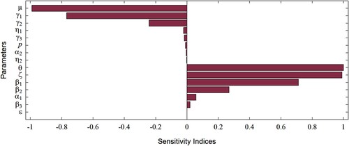
Table 3. Sensitivity indices of the model parameters using differential sensitivity analysis [28].

Parameter (ω)	Sensitivity index ($S_{\omega }$)
ϕ	−18.797
μ	−0.9903
${\gamma }_1$	−0.7686
${\gamma }_2$	−0.2423
${\eta }_1$	−0.0218
${\gamma }_3$	−0.0173
p	−0.0101
${\alpha }_2$	−0.0046
${\eta }_2$	−0.0024
θ	1
ζ *	0.9893
${\text{β}}_1$	0.7114
${\text{β}}_2$	0.2689
${\alpha }_1$	0.0579
${\text{β}}_3$	0.0197
ϵ	0.0003

Note: The parameter values are as in Table 2.*Note that $\zeta =1-\varphi$.

The parameters $\theta ,\zeta ,{\text{β}}_1,{\text{β}}_2,{\alpha }_1,{\text{β}}_3,$ and ϵ have a positive influence on ${\mathcal{R}}_0$, while $\varphi ,\mu ,{\gamma }_1,{\gamma }_2,{\eta }_1,{\gamma }_3,p,{\alpha }_2,$ and ${\eta }_2$ have a negative influence on ${\mathcal{R}}_0$. Further, θ, μ, ϕ, ${\text{β}}_1$, and ${\gamma }_1$ are the most sensitive parameters in the model. However, θ and μ are demography parameters, and are not easily amenable to control measures. Thus, the remaining parameters ϕ, ${\text{β}}_1$, and ${\gamma }_1$ are of greatest interest in our study.

Some of the results from our sensitivity analysis were expected, since they follow from and are consistent with the model formulation. For example, we expected that an increase in recovery rates would lead to a decrease in infections, and hence $S_{{\gamma }_1},S_{{\gamma }_2},\mathrm{a}\mathrm{n}\mathrm{d}{S}_{{\gamma }_3}<0$, which is indeed the case according to the sensitivity analysis. However, our sensitivity analysis also highlighted a less obvious result, namely that $S_{{\alpha }_1}$ takes a positive value, despite the expectation that a higher progression rate from mild to moderate symptoms would lead to a reduction of disease burden as ${\text{β}}_1>{\text{β}}_2$.

4.2. Numerical simulations on vaccination (with constant coverage)

Numerical simulations were performed on the model in order to answer our research questions about disease dynamics. The initial values used for the state variables are $\left(S\right(0),V(0),E(0),I_1(0),I_2(0),I_3(0),R(0\left)\right)=(9999,0,0,1,0,0,0)$. The basic reproduction number of the system, evaluated at the parameter values given in Table 2, is ${\mathcal{R}}_0=1.12$. Since ${\mathcal{R}}_0>1$, this indicates that an outbreak occurs thus causing an epidemic in the community.

Figure 4 shows how the value of ${\mathcal{R}}_0$ changes with different pairs of parameters. As expected, ${\mathcal{R}}_0$ varies as transmission coefficient ${\text{β}}_1$ and the vaccine coverage rate p change, but it is much more sensitive to transmission than coverage, if the coverage is low (i.e. between 0.005 and 0.05) (Figure 4(a)). As long as the vaccine coverage is high enough, ${\mathcal{R}}_0$ increases with increasing transmission, but the vaccine is still sufficient to prevent an epidemic that has a low to moderate transmission coefficient (for mild cases). If vaccine coverage is too low, the transmission coefficient does not matter and any value for ${\text{β}}_1$ (across the range shown) gives rise to an epidemic.

Figure 4. Variation in ${\mathcal{R}}_0$ according to different pairs of parameters. The remaining parameters are fixed as in Table 2. The ranges of parameters were chosen to show the most pertinent model behaviour near the threshold of ${\mathcal{R}}_0=1$. Note that the choice of distinct colours is intended for better illustration of results, and does not mean that ${\mathcal{R}}_0$ has discontinuous jumps. (a) Variation in ${\mathcal{R}}_0$ according to ${\text{β}}_1$ and p. (b) Variation in ${\mathcal{R}}_0$ according to ${\text{β}}_1$ and ϕ. (c) Variation in ${\mathcal{R}}_0$ according to p and ϕ.

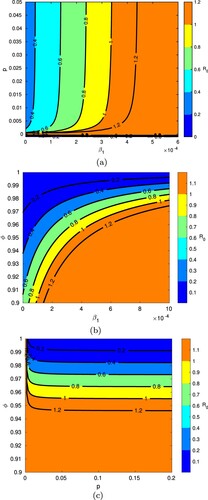
The sensitivity of ${\mathcal{R}}_0$ to transmission coefficient ${\text{β}}_1$ and vaccine efficacy ϕ is shown in Figure 4(b); the greatest variation in results is observed for vaccine efficacies between 90% and 100%. Notice how stronger vaccine efficacies are able to increasingly prevent epidemics with higher values of ${\text{β}}_1$, but lower efficacies are insufficient to control the spread of infection with more moderate or low coefficients of transmission. Looking at vaccine efficacy together with vaccine coverage (Figure 4(c)), notice that efficacies above  96% would be needed to prevent an epidemic across the entire displayed range of vaccine coverage rates (i.e. 0 to 20%).

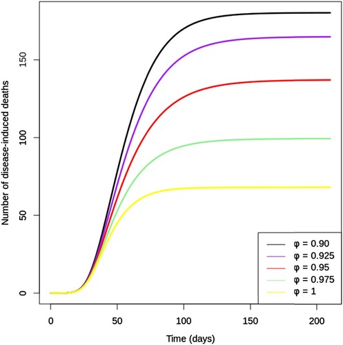
Figure 5 shows the cumulative number of disease-induced deaths over 200 days for different values of vaccine efficacy ($\varphi )$. Notice that the number of deaths after 200 days could be reduced drastically by increasing vaccine efficacy (ϕ) from 90% to 100%. A vaccine with a 97.5% efficacy would save the lives of nearly twice as many infected individuals compared to a vaccine with an efficacy of 90%. Furthermore, it can be observed that a perfect vaccine would reduce the cumulative number of deaths by about 65% as compared to a vaccine which is 90% effective. Therefore, it becomes evident from Figure 5 that high efficacy vaccines considerably reduce disease mortality, even when the vaccine is designed to block infection rather than to reduce disease severity.

Figure 5. Cumulative number of disease-induced deaths given various values of vaccine efficacy (ϕ) between 0.9 and 1. All other parameters are fixed as in Table 2.

4.3. Numerical simulations on vaccine hesitancy

We next use the functional form (2(2) $p=k(1-\psi )\frac{S}{N}.$(2) ) of vaccine coverage to assess the impact of vaccine hesitancy on the spread of infection and the number of disease-induced deaths per day. Figure 6 shows the number of infections (with mild, moderate, and severe symptoms) over time for values of vaccine hesitancy ranging from 0 to 100%. Infections decrease with declining vaccine hesitancy; the peak in mild infections, for example, drops in half (approximately) without vaccine hesitancy ($\psi =0$) as compared to 100% vaccine hesitancy ($\psi =1$, i.e. no vaccination). The peaks of the infection curves shift very slightly to the right as ψ decreases, showing that the time to infection peak is not as rapid without vaccine hesitancy. Notice in Figure 6 that individuals with mild symptoms contribute most to the infection burden. Due to exposed individuals' progression through the three infected stages, with a certain percentage of each infected class being removed from infection, the peak of infections decreases through the progression $I_1\to I_2\to I_3$ (which follows from the model formulation).

Figure 6. Change in (a) $I_1$, (b) $I_2$, and (c) $I_3$ over time with various levels of vaccine hesitancy (ψ) between 0 and 1, with proportionality constant k = 0.05 and vaccine efficacy $\varphi =0.95$. All other parameters are fixed as in Table 2. Note the different scales for the vertical axes. (a) Infections with mild symptoms over time. (b) Infections with moderate symptoms over time. (c) Infections with severe symptoms over time.

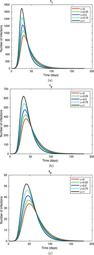
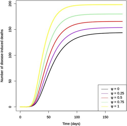
Figure 7 illustrates the cumulative number of disease-induced deaths over 200 days for different values of vaccine hesitancy (ψ). Notice how the predicted cumulative deaths increase evenly as ψ increases from 0 to 100% by quarters. Lower vaccine hesitancy in the community can give rise to epidemics with fewer deaths; the simulation shows that three-quarters as many deaths result from the epidemic with $\psi =1$ as compared to that with $\psi =0$.

Figure 7. Cumulative number of disease-induced deaths given various values of vaccine hesitancy (ψ) between 0 and 1. Note that k = 0.05 and all other parameters are fixed as in Table 2.

4.4. Quantification of results on vaccine hesitancy

In this section, we use simulations to determine the vaccine efficacy needed to reduce the peak of infections by 40% (as compared to the peak in the absence of vaccination), given various levels of vaccine hesitancy. The peak is taken as the maximum value of $I_1$, $I_2$ or $I_3$ (i.e. $I_i^{max}$), and the absence of vaccination is the case where $\psi =1$, and hence p = 0. The value of vaccine efficacy ϕ is then calibrated accordingly (i.e. giving 40% of $I_i^{max}$) with levels of vaccine hesitancy of 10%, 25%, and 60%.

Results are shown in Table 4, revealing the considerable impact of vaccine hesitancy. If 60% of the population is reluctant about being vaccinated, then even a perfect vaccine will not be able to reduce the peaks of infections by 40%. It is interesting to note that even if the vaccine hesitancy is small (10%), the efficacy needs to be above 94% to reduce the peaks of infections by 40%.

Table 4. The vaccine efficacy required to compensate for different levels of vaccine hesitancy.

Vaccine hesitancy (ψ)	Goal	Requirement on vaccine efficacy (ϕ)
10%	Reduce $I_1^{max}$ by 40%	$\varphi =0.93675$
	Reduce $I_2^{max}$ by 40%	$\varphi =0.96704$
	Reduce $I_3^{max}$ by 40%	$\varphi =0.97928$
25%	Reduce $I_1^{max}$ by 40%	$\varphi =0.97090$
	Reduce $I_2^{max}$ by 40%	$\varphi =0.99276$
	Reduce $I_3^{max}$ by 40%	$\varphi =0.99865$
60%	Reduce $I_1^{max}$ by 40%	Infeasible
		($\varphi =1⟹27.57\mathrm{\%}$ drop in $I_1^{max}$)
	Reduce $I_2^{max}$ by 40%	Infeasible
		($\varphi =1⟹25.85\mathrm{\%}$ drop in $I_3^{max}$)
	Reduce $I_3^{max}$ by 40%	Infeasible
		($\varphi =1⟹25.22\mathrm{\%}$ drop in $I_3^{max}$)

Note: Value of peak infection = $I_i^{max}$. Note that k = 0.05 and all other parameters are fixed as in Table 2.

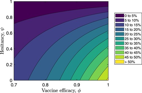
Figure 8 shows how the percentage reduction in the peak of total infections ($I_1+I_2+I_3$) changes as vaccine hesitancy varies from 0 to 100% and vaccine efficacy varies from 70% to 100%. These results suggest that if $\varphi >0.8$ and $\psi <0.6$, the peak of the total infections could be reduced by more than a quarter of the peak infections in the absence of vaccination. It is hence evident that considerable reductions in peak infections could be achieved with lower vaccine hesitancies and much higher vaccine efficacies.

Figure 8. Percentage reductions in the peak of total infection (i.e. the sum $I_1+I_2+I_3$) for varying values of vaccine efficacy (ϕ) and vaccine hesitancy (ψ). All other parameters are fixed as in Table 2.

5. Conclusions

In this study, we developed an SEIR model with vaccination and differential morbidity to gain insights into the epidemiological dynamics of an emerging infectious disease. We also constructed a functional form for vaccine coverage in terms of vaccine hesitancy. The resulting compartmental model of seven state variables expressed as a system of non-linear ODEs was analyzed, both mathematically and numerically. The objectives of the study were to identify how vaccine efficacy and vaccine hesitancy affect disease dynamics; to estimate the efficacy of a vaccine needed to overcome the impact of vaccine hesitancy; to explore how differential morbidity impacts disease dynamics; and to determine which parameters play a pivotal role in an outbreak of disease.

Firstly, we proved some important results on the qualitative nature of the mathematical model. We computed the basic reproduction number (${\mathcal{R}}_0$) of the model using the NGM method. We also proved that the model has a unique endemic equilibrium when ${\mathcal{R}}_0>1$ and no endemic equilibria when ${\mathcal{R}}_0<1$, despite the quadratic equation of endemic equilibria. Then, we performed a bifurcation analysis in order to show that there exists a transcritical bifurcation with respect to ϵ at ${\mathcal{R}}_0=1$.

The numerical analysis of the model involves a sensitivity analysis, graphical simulations, and a quantification of results in order to address the research questions, including the tradeoff between vaccine efficacy and vaccine hesitancy. The sensitivity analysis showed that the parameters that are most sensitive to ${\mathcal{R}}_0$ and easily amenable to control measures are the vaccine efficacy (ϕ) (or vaccine failure (ζ)), transmission coefficient for individuals infected with mild symptoms (${\text{β}}_1$), and recovery rate for individuals infected with mild symptoms (${\gamma }_1$). The sensitivity analysis and Figure 5 indicate that milder infections contribute more to the disease burden; this result follows from the model formulation. Figures 4 and 5 reinforce that more efficacious vaccines could help control the disease burden more efficiently.

In order to examine the impact of vaccine hesitancy on the spread of disease, we performed numerical simulations based on the functional form of p. Figures 6–8 indicate how the disease burden and disease-induced deaths could be decreased with lower vaccine hesitancy. Through the quantification of our results, we established that if the vaccine is not perfect, a lower vaccine hesitancy would be needed to reduce the peaks of infections to the same degree. Thus, it could be inferred that taking steps to overcome vaccine hesitancy could help substantially reduce the disease burden. These results could prove to be useful for healthcare management.

In summary, we used a compartmental epidemiological model of an emerging pathogen to show how the disease burden could be reduced substantially through effective vaccines and reduced vaccine hesitancy levels. Future research in this direction could focus on considering the effects of multiple mutant variants of the pathogen, which could lead to the waning of both vaccine-induced and infection-acquired immunity. Moreover, considering the vaccinated but infected individuals as a separate compartment in the model would enable evaluation of the vaccine efficacy against transmission separately from the vaccine efficacy against severe infections, hospitalizations, and deaths.

Acknowledgments

We would like to thank two anonymous reviewers for feedback that greatly improved our work.

Disclosure statement

No potential conflict of interest was reported by the authors.

Additional information

Funding

Funding from the Simons Foundation (to E.J.S.) is gratefully acknowledged.

References

- World Health Organization. History of smallpox vaccination; n.d. Available from: https://www.who.int/news-room/spotlight/history-of-vaccination/history-of-smallpox-vaccination.
- Centers for Disease Control & Prevention. 14 Diseases you almost forgot about (thanks to vaccines); 2022 Sep 15. Available from: https://www.cdc.gov/vaccines/parents/diseases/forgot-14-diseases.html.
- A. Beukenhorst, C.M. Koch, C. Hadjichrysanthou, et al. SARS-CoV-2 elicits non-Sterilizing immunity and evades vaccine-Induced immunity: implications for future vaccination strategies. Eur J Epidemiol. 2023;38(3):237. doi: 10.1007/s10654-023-00965-x
- Centers for Disease Control & Prevention. Coronavirus disease 2019 (COVID-19); 2020 Feb 11. Available from: https://www.cdc.gov/coronavirus/2019-ncov/science/data-review/vaccines.html.
- World Health Organization. Ten health issues WHO will tackle this year; 2019. Available from: https://www.who.int/news-room/spotlight/ten-threats-to-global-health-in-2019.
- B. Buonomo, R. Della Marca, M. Groppi. A behavioural modelling approach to assess the impact of COVID-19 vaccine hesitancy. J Theor Biol. 2022;534:Article ID 110973. doi: 10.1016/j.jtbi.2021.110973
- E. Dubé, C. Laberge, M. Guay, et al. Vaccine hesitancy. Hum Vaccin Immunother. 2013;9(8):1763–1773. doi: 10.4161/hv.24657
- World Health Organization. Vaccine hesitancy: a growing challenge for immunization programmes; 2015. Available from: https://www.who.int/news/item/18-08-2015-vaccine-hesitancy-a-growing-challenge-for-immunization-programmes.
- World Health Organization. Coronavirus disease (COVID-19): vaccines; n.d. Available from: https://www.who.int/news-room/questions-and-answers/item/coronavirus-disease-(covid-19)-vaccines.
- D. Olivera Mesa, P. Winskill, A.C. Ghani, et al. The societal cost of vaccine refusal: a modelling study using measles vaccination as a case study. Vaccine. 2023;41(28):4129–4137. doi: 10.1016/j.vaccine.2023.05.039
- C.H. Leung, M.E. Gibbs, P.E. Pare. The impact of vaccine hesitancy on epidemic spreading. In: American Control Conference (ACC); 2022, p. 3656–3661. doi: 10.23919/ACC53348.2022.9867327
- B. Oduro, A. Miloua, O.O. Apenteng, et al. COVID-19 vaccination hesitancy model: the impact of vaccine education on controlling the outbreak. Math Model Appl. 2021;6(4):81–91. doi: 10.11648/j.mma.20210604.11
- M. Angeli, G. Neofotistos, M. Mattheakis, et al. Modeling the effect of the vaccination campaign on the COVID-19 pandemic. Chaos Solit Fractals. 2022;154:Article ID 111621. doi: 10.1016/j.chaos.2021.111621
- G. Ledder. Incorporating mass vaccination into compartment models for infectious diseases. medRxiv; 2022. p. 2022.04.26.22274335. doi: 10.1101/2022.04.26.22274335
- A. de Miguel-Arribas, A. Aleta, Y. Moreno. Impact of vaccine hesitancy on secondary COVID-19 outbreaks in the US: an age-structured SIR model. BMC Infect Dis. 2022;22(1):511. doi: 10.1186/s12879-022-07486-0
- Centers for Disease Control & Prevention. COVID-19 and your health. Centers for disease control and prevention; 2020 Feb. Available from: https://www.cdc.gov/coronavirus/2019-ncov/your-health/about-covid-19/basics-covid-19.html.
- E.P. Esteban, L. Almodovar-Abreu. Assessing the impact of vaccination in a COVID-19 compartmental model. Inform Med Unlocked. 2021;27:Article ID 100795. doi: 10.1016/j.imu.2021.100795
- I. Ahmed, G.U. Modu, A. Yusuf, et al. A mathematical model of coronavirus disease (COVID-19) containing asymptomatic and symptomatic classes. Results Phys. 2021 Feb;21:Article ID 103776. doi: 10.1016/j.rinp.2020.103776
- National Institute of Health. Clinical spectrum of SARS-CoV-2 infection; n.d. Available from: https://www.covid19treatmentguidelines.nih.gov/overview/clinical-spectrum/.
- T. Šušteršič, A. Blagojević, D. Cvetković, et al. Epidemiological predictive modeling of COVID-19 infection: development, testing, and implementation on the population of the benelux union. Front Public Health 9 (2021), pp. 1–24. doi:10.3389/fpubh.2021.727274.
- Johns Hopkins Coronavirus Resource Center. Mortality analyses; n.d. Available from: https://coronavirus.jhu.edu/data/mortality.
- C. Kerr, R. Stuart, D. Mistry, et al. Covasim: an agent-Based model of COVID-19 dynamics and interventions. PLoS Comput Biol. 2021 Jul;17(7):e1009149. PLoS Journals. doi: 10.1371/journal.pcbi.1009149
- A. Wilder-Smith. What is the vaccine effect on reducing transmission in the context of the SARS-CoV-2 delta variant? Lancet Infect Dis. 2022 Feb;22(2):152–153. doi: 10.1016/S1473-3099(21)00690-3
- D. Swan, C. Bracis, H. Janes, et al. COVID-19 vaccines that reduce symptoms but do not block infection need higher coverage and faster rollout to achieve population impact. Sci Rep. 2021 Jul 1;11(1):Article ID 15531. doi: 10.1038/s41598-021-94719-y
- Z.S. Kifle, L.L. Obsu. Mathematical modeling for COVID-19 transmission dynamics: a case study in Ethiopia. Results Phys. 2022 Mar;34:Article ID 105191. doi: 10.1016/j.rinp.2022.105191
- J. Mondal, S. Khajanchi. Mathematical modeling and optimal intervention strategies of the COVID-19 outbreak. Nonlinear Dyn. 2022;109(1):177–202. doi: 10.1007/s11071-022-07235-7
- P. Samui, J. Mondal, S. Khajanchi. A mathematical model for COVID-19 transmission dynamics with a case study of India. Chaos Solitons Fractals. 2020 Nov;140:Article ID 110173. doi: 10.1016/j.chaos.2020.110173
- C.W. Castillo-Garsow, C. Castillo-Chavez, A tour of the basic reproductive number and the next generation of researchers, in An Introduction to Undergraduate Research in Computational and Mathematical Biology, H. Callender Highlander, A. Capaldi, and C. Diaz Eaton, ed., Foundations for Undergraduate Research in Mathematics, Birkhäuser, Cham, 2020. doi:10.1007/978-3-030-33645-5_2
- P. van den Driessche, J. Watmough. Reproduction numbers and sub-threshold endemic equilibria for compartmental models of disease transmission. Math Biosci. 2002 Nov;180(1):29–48. doi: 10.1016/S0025-5564(02)00108-6
- O. Diekmann, J.A.P. Heesterbeek, J.A.J. Metz. On the definition and the computation of the basic reproduction ratio R0 in models for infectious diseases in heterogeneous populations. J Math Biol. 1990 Jun;28(4):365–382. doi: 10.1007/BF00178324
- A.B. Gumel. Causes of backward bifurcations in some epidemiological models. J Math Anal Appl. 2012 Nov;395(1):355–365. doi: 10.1016/j.jmaa.2012.04.077
- B. Song. Basic reinfection number and backward bifurcation. Math Biosci Eng. 2021;18(6):8064–8083. mbe-18-06-400. doi: 10.3934/mbe.2021400
- M. Martcheva. Methods for deriving necessary and sufficient conditions for backward bifurcation. J Biol Dyn. 2019;13(1):538–566. doi: 10.1080/17513758.2019.1647359
- C. Castillo-Chavez, B. Song. Dynamical models of tuberculosis and their applications. Math Biosci Eng. 2004;1(2):361–404. doi: 10.3934/mbe.2004.1.361