Optimal control of a multi-scale HIV-opioid model

Abstract

In this study, we apply optimal control theory to an immuno-epidemiological model of HIV and opioid epidemics. For the multi-scale model, we used four controls: treating the opioid use, reducing HIV risk behaviour among opioid users, entry inhibiting antiviral therapy, and antiviral therapy which blocks the viral production. Two population-level controls are combined with two within-host-level controls. We prove the existence and uniqueness of an optimal control quadruple. Comparing the two population-level controls, we find that reducing the HIV risk of opioid users has a stronger impact on the population who is both HIV-infected and opioid-dependent than treating the opioid disorder. The within-host-level antiviral treatment has an effect not only on the co-affected population but also on the HIV-only infected population. Our findings suggest that the most effective strategy for managing the HIV and opioid epidemics is combining all controls at both within-host and between-host scales.

Keywords:

• Basic reproduction number
• opioid epidemic
• HIV
• optimal control
• multi-scale model

Mathematics Subject Classification:

• 92D30

1. Introduction

Over the past two decades, opioid-related deaths in the United States have skyrocketed from nearly 8500 in 2000 to almost 70,000 in 2020 [1]. The US Department of Health and Human Services declared the opioid crisis a nationwide public health emergency in 2017 [2]. The National Institutes of Health (NIH) has indicated a link between the increased number of HIV diagnoses and the rising incidence of opioid disorders [3]. Increased HIV-risk behaviour among opioid users is found to be the primary cause of this association [3].

The opioid epidemic and the HIV epidemic have been extensively modelled as separate epidemics. The early models of the opioid epidemic focussed on heroin. White and Comiskey [4] introduced a simple ODE model with users not in treatment and users in treatment. A number of extensions of this model were also considered. Nyabadza and Hove-Musekwa [5] studied the heroin epidemic in a South African Province. Samanta [6] considered a non-autonomous version of a heroin model while articles [7–9] considered versions with distributed delay(s). Age-structured PDE models were also investigated [10–13]. More recently the attention has turned to answering real-life questions with opioid models. Several articles address the prescription opioids as a vehicle toward illicit drugs or target best treatment strategies [14–17]. Optimal control models have rarely been investigated in the context of the opioid epidemic. The only studies we found are [18,19]. The HIV epidemic has been extensively modelled since its beginning. There are several books devoted to HIV/AIDS epidemic modelling in both deterministic and stochastic settings [20,21]. Optimal control of HIV has also been extensively investigated [22,23].

We have previously introduced several models of HIV and opioid epidemics to better understand their interactions [24–27]. We initially started with a compartmental ODE model of HIV and opioid dynamics [24], and then progressed to a multi-scale model that included both the within-host and between-host dynamics of the two epidemics [25]. Finally, we developed a multi-scale model in which the HIV dynamics are defined on a scale-free network [26]. With both HIV and opioid invasion numbers larger than one, the initial model revealed that the two epidemics are in the coexisting regime in the United States [24]. Elasticities of the invasion numbers indicated that opioid addiction treatment and lowering HIV risk behaviour among opioid users would be the most effective control strategies in decoupling the epidemics [24]. Furthermore, we applied optimal control to the HIV-opioid ODE compartmental model, and obtained similar results [27]. However, using a network multi-scale model of HIV and opioid, without the optimal control, we discovered conflicting conclusions. According to numerical simulations of a network multi-scale model of HIV and opioid, the population of individuals who are both HIV-infected and opioid users, termed as co-affected population, is not monotone with respect to the risk of an opioid user being infected with HIV [26]. We observe that as the risk of opioid users acquiring HIV decreases, the number of co-affected individuals may both increase and decrease. A logical next step in identifying the most effective control measures in managing the two epidemics would be to apply the optimal control theory to the multi-scale model and incorporate controls at both scales.

Optimal control theory has been applied to immuno-epidemiological multi-scale models of HIV before [28–30]. In this study, we introduce an optimal control theory of multi-scale models of two interacting epidemics. We incorporate two control measures at the population scale; treating the opioid addiction and reducing the HIV risk among opioid users. The two population scale controls are combined with two within-host scale control measures; antiviral therapy blocking HIV entry to the target cells and antiviral therapy preventing the infected target cells from producing new HIV particles. The steps proving the existence of optimal control for the first-order PDEs differs from the traditional approaches. Ekeland's Principle [31] allows us to prove the existence of an optimum control of multi-scale immuno-epidemiological models which are first-order PDEs. In Section 2, we introduce the multi-scale immuno-epidemiological model of HIV and opioid, and then incorporate controls to the between-host and within-host models. In Sections 3 and 4, we prove the existence and uniqueness of the optimal control. In Section 5, we present the numerical simulations. In Section 6, we summarize our results.

2. The model and its optimal control version

The states for the epidemic transmission process are divided into susceptible state S, opioid state U, infected with HIV state V, co-affected state $i(\tau ,t)$ and AIDS state A. Individuals change states at rates given by the forces of infection. Susceptible individuals are recruited at the recruitment rate Λ. Susceptible, opioid, infected, co-affected and AIDS individuals leave the system at a natural death rate μ or at disease-induced death rates $d_u$, $d_v$, $d_i\left(\tau \right)$, $d_a$. A susceptible individual can be infected with HIV and change into an infected state, or can become opioid-dependent and change into opioid state. HIV and opioid individuals can get co-affected by adding the other disease. An opioid individual or co-affected individual can move to a susceptible or HIV-infected state respectively due to treatment at a rate δ. HIV-infected or co-affected individuals can move to the AIDS state at rates ${\gamma }_v$ or ${\gamma }_i$.

Let $S\left(t\right)$, $U\left(t\right)$, $V\left(t\right)$, $A\left(t\right)$, be the number of susceptible, opioid-dependent, infected with HIV and AIDS individuals, respectively, at time t, and $i(\tau ,t)$ be the density of co-affected individuals at time t and with co-affection age τ. The co-affection age τ starts when one becomes both infected with HIV and opioid-addicted. Then we formulate the following multi-scale model of HIV and opioid epidemics: (1) $\begin{array}{r}\{\begin{array}{l}{\displaystyle \frac{\mathrm{d}S\left(t\right)}{\mathrm{d}t}=\mathrm{\Lambda }-{\lambda }_u\left(t\right)S\left(t\right)-{\lambda }_v\left(t\right)S\left(t\right)-\mathrm{\mu S}\left(t\right)+\mathrm{\delta U}\left(t\right),}\\ {\displaystyle \frac{\mathrm{d}U\left(t\right)}{\mathrm{d}t}={\lambda }_u\left(t\right)S\left(t\right)-q_v{\lambda }_v\left(t\right)U\left(t\right)-(\mu +d_u+\delta )U\left(t\right),}\\ {\displaystyle \frac{\mathrm{d}V\left(t\right)}{\mathrm{d}t}={\lambda }_v\left(t\right)S\left(t\right)-q_u{\lambda }_u\left(t\right)V\left(t\right)-(\mu +d_v+{\gamma }_v)V\left(t\right)+\delta {\int }_0^{\mathrm{\infty }}\sigma \left(\tau \right)i(t,\tau )\mathrm{d}\tau ,}\\ {\displaystyle \frac{\mathrm{\partial }i(t,\tau )}{\mathrm{d}t}+\frac{\mathrm{\partial }{k}_{s}i(t,\tau )}{\mathrm{d}\tau }=-(\mu +d_i(\tau )+{\gamma }_i(\tau )+\mathrm{\delta \sigma }(\tau \left)\right)i(t,\tau ),}\\ k_{s}i(t,0)=q_v{\lambda }_v\left(t\right)U\left(t\right)+q_u{\lambda }_u\left(t\right)V\left(t\right)\\ {\displaystyle \frac{\mathrm{d}A\left(t\right)}{\mathrm{d}t}={\gamma }_{v}V\left(t\right)+{\int }_0^{\mathrm{\infty }}{\gamma }_i\left(\tau \right)i(t,\tau )\mathrm{d}\tau -(\mu +d_a)A\left(t\right).}\end{array}\end{array}$(1) The total population size is $N\left(t\right)=S\left(t\right)+U\left(t\right)+V\left(t\right)+{\int }_0^{\mathrm{\infty }}i(t,\tau )\mathrm{d}\tau$. We note here that we assume that since AIDS individuals typically suffer from opportunistic illnesses, they are too sick to participate in the population mixing. As a result of this simplifying assumption, the class A is excluded from the total population N, as well as from the force of infection of HIV. The force of HIV infection, ${\lambda }_v\left(t\right)$, is given by: (2) ${\lambda }_v\left(t\right)=\frac{{\text{β}}_{v_1}V\left(t\right)+{\int }_0^{\mathrm{\infty }}{\text{β}}_{v_2}\left(\tau \right)i(t,\tau )\mathrm{d}\tau }{N\left(t\right)}.$(2) Thus, ${\lambda }_v\left(t\right)$ denotes the force of infection of HIV, where ${\text{β}}_{v_1}$ is the transmission coefficient from $V\left(t\right)$. Similarly, ${\text{β}}_{v_2}\left(\tau \right)$ is the time-since-infection dependent transmission coefficient from $i(\tau ,t)$. The force of opioid addiction, ${\lambda }_u\left(t\right)$, is given by (3) ${\lambda }_u\left(t\right)={\text{β}}_u\frac{U\left(t\right)+{\int }_0^{\mathrm{\infty }}i(t,\tau )\mathrm{d}\tau }{N\left(t\right)}.$(3) We assume the addiction coefficient is the same for U and ${\int }_0^{\mathrm{\infty }}i(t,\tau )\mathrm{d}\tau$. We further note that model (1(1) $\begin{array}{r}\{\begin{array}{l}{\displaystyle \frac{\mathrm{d}S\left(t\right)}{\mathrm{d}t}=\mathrm{\Lambda }-{\lambda }_u\left(t\right)S\left(t\right)-{\lambda }_v\left(t\right)S\left(t\right)-\mathrm{\mu S}\left(t\right)+\mathrm{\delta U}\left(t\right),}\\ {\displaystyle \frac{\mathrm{d}U\left(t\right)}{\mathrm{d}t}={\lambda }_u\left(t\right)S\left(t\right)-q_v{\lambda }_v\left(t\right)U\left(t\right)-(\mu +d_u+\delta )U\left(t\right),}\\ {\displaystyle \frac{\mathrm{d}V\left(t\right)}{\mathrm{d}t}={\lambda }_v\left(t\right)S\left(t\right)-q_u{\lambda }_u\left(t\right)V\left(t\right)-(\mu +d_v+{\gamma }_v)V\left(t\right)+\delta {\int }_0^{\mathrm{\infty }}\sigma \left(\tau \right)i(t,\tau )\mathrm{d}\tau ,}\\ {\displaystyle \frac{\mathrm{\partial }i(t,\tau )}{\mathrm{d}t}+\frac{\mathrm{\partial }{k}_{s}i(t,\tau )}{\mathrm{d}\tau }=-(\mu +d_i(\tau )+{\gamma }_i(\tau )+\mathrm{\delta \sigma }(\tau \left)\right)i(t,\tau ),}\\ k_{s}i(t,0)=q_v{\lambda }_v\left(t\right)U\left(t\right)+q_u{\lambda }_u\left(t\right)V\left(t\right)\\ {\displaystyle \frac{\mathrm{d}A\left(t\right)}{\mathrm{d}t}={\gamma }_{v}V\left(t\right)+{\int }_0^{\mathrm{\infty }}{\gamma }_i\left(\tau \right)i(t,\tau )\mathrm{d}\tau -(\mu +d_a)A\left(t\right).}\end{array}\end{array}$(1) ) assumes that individuals can become opioid-addicted only through contact with opioid-addicted person. We do not model the scenario of possible addiction through prescription drugs [14].

For the within-host model of co-affected individuals, we modify a well-known within-host model of HIV [32,33] by explicitly including the opioid drug concentration $C\left(\tau \right)$ and its impact on the average susceptibility of target cells: (4) $\{\begin{array}{l}\begin{array}{rl}{\displaystyle \frac{\mathrm{d}T}{\mathrm{d}\tau }}& =s-d_{T}T-k\left(C\right)V_{i}T,\\ {\displaystyle \frac{\mathrm{d}{T}_i}{\mathrm{d}\tau }}& =k\left(C\right)V_{i}T-{\delta }_i{T}_i,\\ {\displaystyle \frac{\mathrm{d}{V}_i}{\mathrm{d}\tau }}& =N_v{\delta }_i{T}_i-c{V}_i,\\ {\displaystyle \frac{\mathrm{d}C}{\mathrm{d}\tau }}& =-d_{c}C,\\ C\left({\tau }_j^{+}\right)& =C\left({\tau }_j^{-}\right)+D.\end{array}\end{array}$(4) Here, T are the healthy target cells, $T_i$ are the infected target cells and $V_i$ is the virus (HIV). Target cells are produced at rate s and cleared at rate $d_T$. Infected cells die at a rate ${\delta }_i$, and when they die, they release $N_v$ viral particles at bursting. The clearance rate of the virus is denoted by c. In our model, opioid is taken at doses D at times ${\tau }_j,j=1,2,\dots ,$ and it is degraded at rate $d_c$. Infection rate of target cells by HIV in the presence of opioid is given by $k\left(C\right)=\frac{k_{1}C\left(\tau \right)}{C_0+C\left(\tau \right)},$where $C_0$ is the half-saturation constant and $k_1$ is a maximal increase in infection rate due to opioids. The resulting within-host model is a pharmacokinetic type of model. It is an impulsive model, where ${\tau }_j^{+}$ and ${\tau }_j^{-}$ represent the right and left limit, respectively.

In order to link the within-host and between-host models, we use data in [34] to determine the form of the linking of the transmission coefficient ${\text{β}}_{v_2}\left(\tau \right)$ to the viral load [35]. Fitting to the data, we obtain the following function for ${\text{β}}_{v_2}\left(\tau \right)$: ${\text{β}}_{v_2}\left(\tau \right)=\frac{{\text{β}}_0{V}_i^r\left(\tau \right)}{B+V_i^r\left(\tau \right)},$where $r\approx 1$. Further, we use the suggested functions in [36] to link the remaining τ-dependent rates: $d_i\left(\tau \right)=d_0\left(T\right(0)-T(\tau \left)\right),{\gamma }_i\left(\tau \right)={\gamma }_0\left(T\right(0)-T(\tau \left)\right),\sigma \left(\tau \right)={\sigma }_0,$where $d_0,{\sigma }_0,{\text{β}}_0,{\gamma }_0,B$ are given constants. The disease-induced death rate, $d_i$, of co-affected individuals and their transition rate, ${\gamma }_i$, to AIDS does not depend explicitly on the viral load because the viral load is high during the acute HIV phase but the rates ${\gamma }_i\left(\tau \right)$ and $d_i\left(\tau \right)$ are not correspondingly high during the acute HIV stage. Because $d_i$ and ${\gamma }_i$ must be small during the acute HIV stage when the viral load is very high, reference [36] suggests that they depend on the target cells instead. Thus, we adopt the suggested form from reference [36]. For simplicity, we choose $\sigma \left(\tau \right)$ as a constant which gives the fraction of co-affected individuals successfully treated.

Our prior results suggested two foci for control measures: targeting the drug abuse epidemic and reducing HIV risk in drug-users. As a part of this paper, we will compare and contrast these foci of control, obtained from elasticity analysis, with time-dependent optimal control strategies. Optimal control has been applied in the past to multi-scale HIV models [28,29,37–39], but to the best of our knowledge, it has not been applied to a multi-scale model with two diseases. CDC [40] lists the control measures for HIV, with the most effective measure being the antiretroviral therapy (ART). Multiple control measures might affect HIV risk in drug users (e.g. preexposure prophylaxis, education for condom use, availability of free syringes for injecting drug users). All these measures decrease the parameter $q_v$. We include treatment of opioid users in our model in the form of the parameter δ. Let $u_1\left(t\right)$ be the control variable corresponding to the treatment parameter δ and $u_2\left(t\right)$ encompass control measures that reduce the HIV-risk behaviours in drug users, then the between-host component of the multi-scale model (1(1) $\begin{array}{r}\{\begin{array}{l}{\displaystyle \frac{\mathrm{d}S\left(t\right)}{\mathrm{d}t}=\mathrm{\Lambda }-{\lambda }_u\left(t\right)S\left(t\right)-{\lambda }_v\left(t\right)S\left(t\right)-\mathrm{\mu S}\left(t\right)+\mathrm{\delta U}\left(t\right),}\\ {\displaystyle \frac{\mathrm{d}U\left(t\right)}{\mathrm{d}t}={\lambda }_u\left(t\right)S\left(t\right)-q_v{\lambda }_v\left(t\right)U\left(t\right)-(\mu +d_u+\delta )U\left(t\right),}\\ {\displaystyle \frac{\mathrm{d}V\left(t\right)}{\mathrm{d}t}={\lambda }_v\left(t\right)S\left(t\right)-q_u{\lambda }_u\left(t\right)V\left(t\right)-(\mu +d_v+{\gamma }_v)V\left(t\right)+\delta {\int }_0^{\mathrm{\infty }}\sigma \left(\tau \right)i(t,\tau )\mathrm{d}\tau ,}\\ {\displaystyle \frac{\mathrm{\partial }i(t,\tau )}{\mathrm{d}t}+\frac{\mathrm{\partial }{k}_{s}i(t,\tau )}{\mathrm{d}\tau }=-(\mu +d_i(\tau )+{\gamma }_i(\tau )+\mathrm{\delta \sigma }(\tau \left)\right)i(t,\tau ),}\\ k_{s}i(t,0)=q_v{\lambda }_v\left(t\right)U\left(t\right)+q_u{\lambda }_u\left(t\right)V\left(t\right)\\ {\displaystyle \frac{\mathrm{d}A\left(t\right)}{\mathrm{d}t}={\gamma }_{v}V\left(t\right)+{\int }_0^{\mathrm{\infty }}{\gamma }_i\left(\tau \right)i(t,\tau )\mathrm{d}\tau -(\mu +d_a)A\left(t\right).}\end{array}\end{array}$(1) ) with optimal control takes the form: (5) $\{\begin{array}{l}{\displaystyle \frac{\mathrm{d}S\left(t\right)}{\mathrm{d}t}=\mathrm{\Lambda }-{\lambda }_u\left(t\right)S\left(t\right)-{\lambda }_v\left(t\right)S\left(t\right)-\mathrm{\mu S}\left(t\right)+\delta u_1\left(t\right)U\left(t\right),}\\ {\displaystyle \frac{\mathrm{d}U\left(t\right)}{\mathrm{d}t}={\lambda }_u\left(t\right)S\left(t\right)-q_v(1-u_2(t\left)\right){\lambda }_v\left(t\right)U\left(t\right)-(\mu +d_u+\delta u_1(t\left)\right)U\left(t\right),}\\ {\displaystyle \frac{\mathrm{d}V\left(t\right)}{\mathrm{d}t}={\lambda }_v\left(t\right)S\left(t\right)-q_u{\lambda }_u\left(t\right)V\left(t\right)-(\mu +d_v+{\gamma }_v)V\left(t\right)}\\ +\delta u_1\left(t\right){\displaystyle {\int }_0^{\mathrm{\infty }}\sigma \left(\tau \right)i(t,\tau )\mathrm{d}\tau ,}\\ {\displaystyle \frac{\mathrm{\partial }i(t,\tau )}{\mathrm{d}t}+\frac{\mathrm{\partial }{k}_{s}i(t,\tau )}{\mathrm{d}\tau }=-(\mu +d_i(\tau )+{\gamma }_i(\tau )+\sigma (\tau \left)\delta u_1\right(t\left)\right)i(t,\tau ),}\\ k_{s}i(t,0)=q_v(1-u_2(t\left)\right){\lambda }_v\left(t\right)U\left(t\right)+q_u{\lambda }_u\left(t\right)V\left(t\right)\\ {\displaystyle \frac{\mathrm{d}A\left(t\right)}{\mathrm{d}t}={\gamma }_{v}V\left(t\right)+{\int }_0^{\mathrm{\infty }}{\gamma }_i\left(\tau \right)i(t,\tau )\mathrm{d}\tau -(\mu +d_A)A\left(t\right),}\end{array}$(5) where the forces of infection (addiction) remain unchanged. Since the equation for the AIDS individuals, A, is not connected to the rest of the systems, we can omit it in our further analysis. Thus, we will consider the following between-host system (6) $\{\begin{array}{l}{\displaystyle \frac{\mathrm{d}S\left(t\right)}{\mathrm{d}t}=\mathrm{\Lambda }-{\lambda }_u\left(t\right)S\left(t\right)-{\lambda }_v\left(t\right)S\left(t\right)-\mathrm{\mu S}\left(t\right)+\delta u_1\left(t\right)U\left(t\right),}\\ {\displaystyle \frac{\mathrm{d}U\left(t\right)}{\mathrm{d}t}={\lambda }_u\left(t\right)S\left(t\right)-q_v(1-u_2(t\left)\right){\lambda }_v\left(t\right)U\left(t\right)-(\mu +d_u+\delta u_1(t\left)\right)U\left(t\right),}\\ {\displaystyle \frac{\mathrm{d}V\left(t\right)}{\mathrm{d}t}={\lambda }_v\left(t\right)S\left(t\right)-q_u{\lambda }_u\left(t\right)V\left(t\right)-(\mu +d_v+{\gamma }_v)V\left(t\right)}\\ {\displaystyle +\delta u_1\left(t\right){\int }_0^{\mathrm{\infty }}\sigma \left(\tau \right)i(t,\tau )\mathrm{d}\tau ,}\\ {\displaystyle \frac{\mathrm{\partial }i(t,\tau )}{\mathrm{d}t}+\frac{\mathrm{\partial }{k}_{s}i(t,\tau )}{\mathrm{d}\tau }=-(\mu +d_i(\tau )+{\gamma }_i(\tau )+\sigma (\tau \left)\delta u_1\right(t\left)\right)i(t,\tau ),}\\ k_{s}i(t,0)=q_v(1-u_2(t\left)\right){\lambda }_v\left(t\right)U\left(t\right)+q_u{\lambda }_u\left(t\right)V\left(t\right).\end{array}$(6) We also include controls that mimic HIV treatment in the within-host model: (7) $\{\begin{array}{l}\begin{array}{rl}{\displaystyle \frac{\mathrm{d}T}{\mathrm{d}\tau }}& =s-d_{T}T-k\left(C\right)(1-u_3(\tau \left)\right)V_{i}T,\\ {\displaystyle \frac{\mathrm{d}{T}_i}{\mathrm{d}\tau }}& =k\left(C\right)(1-u_3(\tau \left)\right)V_{i}T-{\delta }_i{T}_i,\\ {\displaystyle \frac{\mathrm{d}{V}_i}{\mathrm{d}\tau }}& =N_v{\delta }_i(1-u_4(\tau \left)\right)T_i-c{V}_i,\\ {\displaystyle \frac{\mathrm{d}C}{\mathrm{d}\tau }}& =D-d_{c}C,\end{array}\end{array}$(7) where the coefficient $1-u_3\left(t\right)$ represents the drug effect that reduces transmission of healthy cells to infected cells as a result of interaction with the virus, while the coefficient $1-u_4\left(t\right)$ gives the effect of another drug that reduces the production of viral particles. We implicitly assume here that all co-affected individuals are subject to the same treatment regimen. We have modelled opioid intake with a simpler model of constant intake which tracks the average change in the concentration very well while removing the oscillation of an impulsive model. All controls are assumed bounded: $0\le u_l\left(t\right)\le u_{lmax}$ for $l=1,\dots ,4$. The controls will be determined to minimize the number of HIV-infected individuals and opioid users as well as the cost of implementing the control. The objective functional for control problem is: (8) $\begin{array}{rl}\mathcal{J}\left(\mathbf{u}\right)& ={\int }_0^{t_f}\left[A_{1}U\right(t)+A_{2}V(t)+A_3{\int }_0^{{\tau }_f}i(\tau ,t\left)\mathrm{d}\tau \right]\mathrm{d}t\\ & +{\int }_0^{t_f}(A_4{u}_1\left(t\right)U\left(t\right)+B_1{u}_1^2(t)+B_2{u}_2^2(t\left)\right)\mathrm{d}t\\ & +{\int }_0^{{\tau }_f}\left(B_3{u}_3^2\right(\tau )+B_4{u}_4^2(\tau \left)\right)\mathrm{d}\tau ,\end{array}$(8) where $A_1$, $A_2$, $A_3$,$A_4$, and $B_k$, k = 1, 2, 3, 4, are positive constants that balance the relative importance for the terms in $\mathcal{J}$. In our objective functional, the first term with the A coefficients represents the total of the diseased individuals over time to be minimized and the term with the B coefficients represent the costs of implementing the controls. We note that we assume that the AIDS individuals in the class A are not mixing in the population and they do not affect the transmission of HIV. Hence, we do not include them in the cost functional since reducing their numbers does not affect HIV prevalence significantly. In principle, we want to keep our cost functional $\mathcal{J}$ as simple as possible but it can certainly include other useful terms. In Equation (8(8) $\begin{array}{rl}\mathcal{J}\left(\mathbf{u}\right)& ={\int }_0^{t_f}\left[A_{1}U\right(t)+A_{2}V(t)+A_3{\int }_0^{{\tau }_f}i(\tau ,t\left)\mathrm{d}\tau \right]\mathrm{d}t\\ & +{\int }_0^{t_f}(A_4{u}_1\left(t\right)U\left(t\right)+B_1{u}_1^2(t)+B_2{u}_2^2(t\left)\right)\mathrm{d}t\\ & +{\int }_0^{{\tau }_f}\left(B_3{u}_3^2\right(\tau )+B_4{u}_4^2(\tau \left)\right)\mathrm{d}\tau ,\end{array}$(8) ), $t_f$ and ${\tau }_f$ are the final times for the control. The optimal control problem that we will be solving is: Find $(u_1,u_2,u_3,u_4)\in \mathcal{U}$ such that $\mathcal{J}(u_1^{\ast },u_2^{\ast },u_3^{\ast },u_4^{\ast })=\underset{(u_1,u_2,u_3,u_4)\in \mathcal{U}}{min}\mathcal{J}(u_1,u_2,u_3,u_4),$where the control set $\mathcal{U}$ is $\begin{array}{rl}\mathcal{U}& =\left\{\right(u_1,u_2,u_3,u_4)\in X|u_1,u_2:(0,t_f)\to [0,u_{i,max}],\\ & i=1,2;u_3,u_4:(0,{\tau }_f)\to [0,u_{jmax}],j=3,4\}\end{array}$and X is the space $X=\left(L^{\mathrm{\infty }}\right(0,t_f){)}^2\times (L^{\mathrm{\infty }}(0,{\tau }_f){)}^2$. This optimal control problem is novel because it involves both within-host and between-host controls and two-disease structure. In principle, the controls $\mathbf{u}$ are $L^1$ controls and have to be handled differently than controls in Hilbert spaces. In particular, to obtain the adjoint system, we first define a system of sensitivities [28,29]. After we derive the adjoint system, we characterize the optimal control quadruple and use a modified forward-backward sweep method [28,41] to solve the system numerically. Our two foci for control are modelled by controls $u_1$ and $u_2$, so we can compare our two focal control strategies to other control strategies such as applying ART only, or applying ART for those with HIV and treatment for drug users but not targeting HIV risk for the latter. In the context of the multi-scale control problem, this means not using control $u_2$. Thus, contrasting our baseline control strategy to other optimal control strategies will help evaluate its promise in public health.

3. The system of sensitivities and the adjoint problem

We prove the Lipschitz property for the state variables as depending on the control functions $u_1,u_2,u_3,u_4$. This property is used to show the existence of the sensitivities as well as the existence and uniqueness of the optimal control.

Theorem 3.1

The map $(u_1,u_2,u_3,u_4)\to (T,T_i,V_i,C,S,U,V,i)(u_1,u_2,u_3,u_4)$ is Lipschitz on the set $\begin{array}{rl}Y& =\left\{\right(T,T_i,V_i,C,S,U,V,i)\in [L^{\mathrm{\infty }}(0,{\tau }_f){]}^4\times \left[L^{\mathrm{\infty }}\right(0,t_f){]}^3\\ & \times L^{\mathrm{\infty }}(0,t_f;L^1(0,{\tau }_f\left)\right):S\ge ϵ>0\}\end{array}$in the following way: $\begin{array}{rl}& \left(\mathrm{i}\right){\int }_0^{{\tau }_f}(|T-\overline{T}|+|T_i-{\overline{T}}_i|+|V_i-{\overline{V}}_i|+|C-\overline{C}|\mathrm{d}\tau \\ & +{\int }_0^{t_f}|S-\overline{S}|+|U-\overline{U}|+|V-\overline{V}|\mathrm{d}t+{\int }_0^{t_f}{\int }_0^{{\tau }_f}|i-\overline{i}|\mathrm{d}\tau \mathrm{d}t\\ & \le C_f({\int }_0^{t_f}|u_1-{\overline{u}}_1|+|u_2-{\overline{u}}_2|\mathrm{d}t+{\int }_0^{{\tau }_f}|u_3-{\overline{u}}_3|+|u_4-{\overline{u}}_4|\mathrm{d}\tau ).\\ & \left(\mathrm{ii}\right)\Vert T-\overline{T}{\Vert }_{L^{\mathrm{\infty }}(0,{\tau }_f)}+\Vert T_i-{\overline{T}}_i{\Vert }_{L^{\mathrm{\infty }}(0,{\tau }_f)}+\Vert V_i-{\overline{V}}_i{\Vert }_{L^{\mathrm{\infty }}(0,{\tau }_f)}+\Vert C-\overline{C}{\Vert }_{L^{\mathrm{\infty }}(0,{\tau }_f)}\\ & +\Vert S-\overline{S}{\Vert }_{L^{\mathrm{\infty }}(0,t_f)}+\Vert U-\overline{U}{\Vert }_{L^{\mathrm{\infty }}(0,t_f)}\\ & +\Vert V-\overline{V}{\Vert }_{L^{\mathrm{\infty }}(0,t_f)}+\Vert i-\overline{i}{\Vert }_{L^{\mathrm{\infty }}(0,t_f)\times L^{\mathrm{\infty }}(0,{\tau }_f)}\\ & \le {\overline{C}}_f(\Vert u_1-{\overline{u}}_1{\Vert }_{L^{\mathrm{\infty }}(0,t_f)}+\Vert u_2-{\overline{u}}_2{\Vert }_{L^{\mathrm{\infty }}(0,t_f)}\\ & +\Vert u_3-{\overline{u}}_3{\Vert }_{L^{\mathrm{\infty }}(0,{\tau }_f)}+\Vert u_4-{\overline{u}}_4{\Vert }_{L^{\mathrm{\infty }}(0,{\tau }_f)}).\end{array}$

Proof.

1. We begin by showing the inequalities for the within-host system. First, we establish the Lipshitz property for $k\left(C\right)$. We have $|k\left(C\right)-k\left(\overline{C}\right)|=|k^{\mathrm{\prime }}\left(\xi \right)||C-\overline{C}|$where $\xi \in (C,\overline{C})$. We have: $|k^{\mathrm{\prime }}\left(\xi \right)|\le \frac{k_1{C}_0}{(C_0+\xi {)}^2}\le \kappa ,$where κ is a constant independent of C. Subtracting the differential equations for T and $\overline{T}$, we have $\begin{array}{rl}\frac{d(T-\overline{T})}{\mathrm{d}t}& =-d_T(T-\overline{T})-k\left(C\right)(1-u_3)V_{i}T+k\left(\overline{C}\right)(1-{\overline{u}}_3){\overline{V}}_i\overline{T}\\ & =-d_T(T-\overline{T})-\left(k\right(C)-k(\overline{C}\left)\right)(1-u_3)V_{i}T-k\left(\overline{C}\right)({\overline{u}}_3-u_3)V_{i}T\\ & -k\left(\overline{C}\right)(1-{\overline{u}}_3)(V_i-{\overline{V}}_i)T-k\left(\overline{C}\right)(1-{\overline{u}}_3){\overline{V}}_i(T-\overline{T}).\end{array}$Integrating from $(0,\tau )$ and using $L^{\mathrm{\infty }}$ bounds on the states, we have (9) $|T-\overline{T}|\left(\tau \right)\le C_1{\int }_0^{{\tau }_f}|u_3-{\overline{u}}_3|\mathrm{d}s+C_2{\int }_0^{\tau }|T-\overline{T}|+|V_i-{\overline{V}}_i|+|C-\overline{C}|\mathrm{d}s.$(9) Similarly, we have (10) $\begin{array}{rl}|T_i-{\overline{T}}_i|\left(\tau \right)& \le C_1{\int }_0^{{\tau }_f}|u_3-{\overline{u}}_3|\mathrm{d}s+C_3{\int }_0^{\tau }|T-\overline{T}|\\ & +|T_i-{\overline{T}}_i|+|V_i-{\overline{V}}_i|+|C-\overline{C}|\mathrm{d}s.\end{array}$(10) (11) $\begin{array}{rl}|V_i-{\overline{V}}_i|\left(\tau \right)& \le C_4{\int }_0^{{\tau }_f}|u_4-{\overline{u}}_4|\mathrm{d}s+C_5{\int }_0^{\tau }|T_i-{\overline{T}}_i|+|V_i-{\overline{V}}_i|\mathrm{d}s\\ |C-\overline{C}|\left(\tau \right)& \le d_c{\int }_0^{\tau }|C-\overline{C}|\mathrm{d}s.\end{array}$(11) Combining Equations (9(9) $|T-\overline{T}|\left(\tau \right)\le C_1{\int }_0^{{\tau }_f}|u_3-{\overline{u}}_3|\mathrm{d}s+C_2{\int }_0^{\tau }|T-\overline{T}|+|V_i-{\overline{V}}_i|+|C-\overline{C}|\mathrm{d}s.$(9) )–(11(11) $\begin{array}{rl}|V_i-{\overline{V}}_i|\left(\tau \right)& \le C_4{\int }_0^{{\tau }_f}|u_4-{\overline{u}}_4|\mathrm{d}s+C_5{\int }_0^{\tau }|T_i-{\overline{T}}_i|+|V_i-{\overline{V}}_i|\mathrm{d}s\\ |C-\overline{C}|\left(\tau \right)& \le d_c{\int }_0^{\tau }|C-\overline{C}|\mathrm{d}s.\end{array}$(11) ), we have $\begin{array}{rl}& (|T-\overline{T}|+|T_i-{\overline{T}}_i|+|V_i-{\overline{V}}_i|+|C-\overline{C}|)\left(\tau \right)\\ & \le C_6{\int }_0^{{\tau }_f}|u_3-{\overline{u}}_3|+|u_4-{\overline{u}}_4|\mathrm{d}s+C_7{\int }_0^{\tau }|T-\overline{T}|\\ & +|T_i-{\overline{T}}_i|+|V_i-{\overline{V}}_i|+|C-\overline{C}|\mathrm{d}s.\end{array}$ Applying Gronwall's inequality, we have (12) $\begin{array}{rl}& (|T-\overline{T}|+|T_i-{\overline{T}}_i|+|V_i-{\overline{V}}_i|+|C-\overline{C}|)\left(\tau \right)\\ & \le C_6(1+C_7{\tau }_f{\mathrm{e}}^{C_7{\tau }_f}){\int }_0^{{\tau }_f}|u_3-{\overline{u}}_3|+|u_4-{\overline{u}}_4|\mathrm{d}s.\end{array}$(12) Integrating both sides of Equation (12(12) $\begin{array}{rl}& (|T-\overline{T}|+|T_i-{\overline{T}}_i|+|V_i-{\overline{V}}_i|+|C-\overline{C}|)\left(\tau \right)\\ & \le C_6(1+C_7{\tau }_f{\mathrm{e}}^{C_7{\tau }_f}){\int }_0^{{\tau }_f}|u_3-{\overline{u}}_3|+|u_4-{\overline{u}}_4|\mathrm{d}s.\end{array}$(12) ), we have (13) $\begin{array}{rl}& {\int }_0^{{\tau }_f}|T-\overline{T}|+|T_i-{\overline{T}}_i|+|V_i-{\overline{V}}_i|+|C-\overline{C}|\left)\right(\tau )\mathrm{d}\tau \\ & \le C_6{\tau }_f(1+C_7{\tau }_f{\mathrm{e}}^{C_7{\tau }_f}){\int }_0^{{\tau }_f}|u_3-{\overline{u}}_3|+|u_4-{\overline{u}}_4|\mathrm{d}s.\end{array}$(13) Next, we consider the between-host system. First, we show the Lipschitz property for the forces of infection ${\lambda }_u$ and ${\lambda }_v$. $\begin{array}{rl}{\lambda }_v-{\overline{\lambda }}_v& =\frac{{\text{β}}_{v_1}V+{\int }_0^{{\tau }_f}{\text{β}}_{v_2}\left(\tau \right)i(\tau ,t)\mathrm{d}\tau }{N}-\frac{{\text{β}}_{v_1}\overline{V}+{\int }_0^{{\tau }_f}{\overline{\text{β}}}_{v_2}\left(\tau \right)\overline{i}(\tau ,t)\mathrm{d}\tau }{\overline{N}}\\ & =\frac{{\text{β}}_{v_1}V+{\int }_0^{{\tau }_f}{\text{β}}_{v_2}\left(\tau \right)i(\tau ,t)\mathrm{d}\tau }{N\overline{N}}(\overline{N}-N)+\frac{{\text{β}}_{v_1}(V-\overline{V})}{\overline{N}}\\ & +\frac{1}{\overline{N}}{\int }_0^{{\tau }_f}{\text{β}}_{v_2}\left(\tau \right)(i-\overline{i})\mathrm{d}\tau +\frac{1}{\overline{N}}{\int }_0^{{\tau }_f}({\text{β}}_{v_2}-{\overline{\text{β}}}_{v_2})\overline{i}\mathrm{d}\tau \end{array}$ We recall $S,\overline{S}>ϵ$ since they belong to Y and hence $N,\overline{N}>ϵ$. Further, $i(\tau ,t)\le \{\begin{array}{ll}i(0,t-\tau ){\pi }_1\left(\tau \right)& \tau <t\\ {\displaystyle i_0(\tau -t)\frac{{\pi }_1\left(\tau \right)}{{\pi }_1(\tau -t)}}& \tau >t,\end{array}$where ${\pi }_1\left(\tau \right)={\mathrm{e}}^{-{\int }_0^{\tau }(\mu +{\gamma }_i(\xi )+d_i(\xi \left)\right)\mathrm{d}\xi }.$It is not hard to see that $|i(0,t-\tau )|<K$, where K is a constant and therefore $|i(\tau ,t)|\le K_1$ for all $\tau \in [0,{\tau }_f]$ and $t\in [0,t_f]$ and all $i_0(\cdot )\le K_1$. Hence, $\begin{array}{rl}|{\lambda }_v-{\overline{\lambda }}_v|& \le C_{10}(|S-\overline{S}|+|U-\overline{U}|+|V-\overline{V}|)+C_{11}{\int }_0^{{\tau }_f}|i-\overline{i}|\mathrm{d}\tau \\ & +C_{12}{\int }_0^{{\tau }_f}|V_i-{\overline{V}}_i|\mathrm{d}\tau ).\end{array}$ Similarly, we can show that $|{\lambda }_u-{\overline{\lambda }}_u|\le C_{13}(|S-\overline{S}|+|U-\overline{U}|+|V-\overline{V}|)+C_{11}{\int }_0^{{\tau }_f}|i-\overline{i}|\mathrm{d}\tau .$Next, we derive inequalities for the between host state variables. In particular, we have (14) $\begin{array}{rl}|S-\overline{S}|& \le C_{20}{\int }_0^t|S-\overline{S}|+|U-\overline{U}|+|V-\overline{V}|+{\int }_0^{{\tau }_f}|i-\overline{i}|\mathrm{d}\tau \mathrm{d}s\\ & +C_{21}{\int }_0^t|u_1-{\overline{u}}_1|\mathrm{d}s+C_{22}{\int }_0^{{\tau }_f}|V_i-{\overline{V}}_i|\mathrm{d}\tau .\end{array}$(14) Similarly, we have (15) $\begin{array}{rl}|U-\overline{U}|& \le C_{25}{\int }_0^t|S-\overline{S}|+|U-\overline{U}|+|V-\overline{V}|+{\int }_0^{{\tau }_f}|i-\overline{i}|\mathrm{d}\tau \mathrm{d}s\\ & +C_{26}{\int }_0^t|u_1-{\overline{u}}_1|+|u_2-{\overline{u}}_2|\mathrm{d}s+C_{27}{\int }_0^{{\tau }_f}|V_i-{\overline{V}}_i|\mathrm{d}\tau .\\ |V-\overline{V}|& \le C_{30}{\int }_0^t|S-\overline{S}|+|U-\overline{U}|+|V-\overline{V}|+{\int }_0^{{\tau }_f}|i-\overline{i}|\mathrm{d}\tau \mathrm{d}s\\ & +C_{31}{\int }_0^t|u_1-{\overline{u}}_1|\mathrm{d}s+C_{32}{\int }_0^{{\tau }_f}|V_i-{\overline{V}}_i|\mathrm{d}\tau ,\end{array}$(15) where we have taken into account that $\sigma \left(\tau \right)={\sigma }_0$. Integrating the partial differential equation to obtain $i(\tau ,t)$, we get $i(\tau ,t)=\{\begin{array}{ll}B(t-\tau ){\mathrm{e}}^{-{\int }_0^{\tau }\mu +{\gamma }_i(\tau -\xi )+d_i(\tau -\xi )+\sigma (\tau -\xi )\delta u_1(t-\xi )\mathrm{d}\xi }& \tau <t\\ i_0(\tau -t){\mathrm{e}}^{-{\int }_0^t\mu +{\gamma }_i(\tau -\xi )+d_i(\tau -\xi )+\sigma (\tau -\xi )\delta u_1(t-\xi )\mathrm{d}\xi }& \tau >t,\end{array}$where $B\left(t\right):=i(0,t)$. To show the Lipschitz condition for the exponents, which depend on the within-host variables as well as the control, we use the following inequality. For $x,y\ge 0$, we have $|{\mathrm{e}}^{-x}-{\mathrm{e}}^{-y}|\le |x-y|.$Hence, $\begin{array}{rl}& |{\mathrm{e}}^{-{\int }_0^t\mu +{\gamma }_i(\tau -\xi )+d_i(\tau -\xi )+{\sigma }_0\delta u_1(t-\xi )\mathrm{d}\xi }-{\mathrm{e}}^{-{\int }_0^t\mu +{\overline{\gamma }}_i(\tau -\xi )+{\overline{d}}_i(\tau -\xi )+{\sigma }_0\delta {\overline{u}}_1\left(\mathrm{t\xi }\right)\mathrm{d}\xi }|\\ & \le {\int }_0^t|{\gamma }_i-{\overline{\gamma }}_i|(\tau -\xi )+|d_i-{\overline{d}}_i|(\tau -\xi )+{\sigma }_0|u_1-{\overline{u}}_1|(t-\xi )\mathrm{d}\xi \\ & \le (d_0+{\gamma }_0){\int }_0^t|T-\overline{T}|(\tau -\xi )\mathrm{d}\xi +{\sigma }_0\delta {\int }_0^t|u_1-{\overline{u}}_1|\left(s\right)\mathrm{d}s.\end{array}$Similarly, $\begin{array}{rl}& |{\mathrm{e}}^{-{\int }_0^{\tau }\mu +{\gamma }_i(\tau -\xi )+d_i(\tau -\xi )+{\sigma }_0\delta u_1(t-\xi )\mathrm{d}\xi }-{\mathrm{e}}^{-{\int }_0^{\tau }\mu +{\overline{\gamma }}_i(\tau -\xi )+{\overline{d}}_i(\tau -\xi )+{\sigma }_0\delta {\overline{u}}_1\left(\mathrm{t\xi }\right)\mathrm{d}\xi }|\\ & \le {\int }_0^{\tau }|{\gamma }_i-{\overline{\gamma }}_i|(\tau -\xi )+|d_i-{\overline{d}}_i|(\tau -\xi )+{\sigma }_0|u_1-{\overline{u}}_1|(t-\xi )\mathrm{d}\xi \\ & \le (d_0+{\gamma }_0){\int }_0^{\tau }|T-\overline{T}|(\tau -\xi )\mathrm{d}\xi +{\sigma }_0\delta {\int }_0^{\tau }|u_1-{\overline{u}}_1|(t-\xi )\mathrm{d}\xi .\end{array}$Thus, $\begin{array}{rl}& {\int }_t^{{\tau }_f}|i-\overline{i}|\mathrm{d}\tau \\ & ={\int }_t^{{\tau }_f}{i}_0(\tau -t)(|{\mathrm{e}}^{-{\int }_0^t\mu +{\gamma }_i(\tau -\xi )+d_i(\tau -\xi )+{\sigma }_0\delta u_1(t-\xi )\mathrm{d}\xi }\\ & -{\mathrm{e}}^{-{\int }_0^t\mu +{\overline{\gamma }}_i(\tau -\xi )+{\overline{d}}_i(\tau -\xi )+{\sigma }_0\delta {\overline{u}}_1\left(\mathrm{t\xi }\right)\mathrm{d}\xi }|)\mathrm{d}\tau \\ & \le {\int }_t^{{\tau }_f}{i}_0(\tau -t)\left[\right(d_0+{\gamma }_0){\int }_0^{\tau }|T-\overline{T}|(s)\mathrm{d}s+{\sigma }_0\delta {\int }_0^t|u_1-{\overline{u}}_1|(s\left)\mathrm{d}s\right]\mathrm{d}\tau \\ & \le C_{50}{\int }_0^{{\tau }_f}|T-\overline{T}|\left(s\right)\mathrm{d}s+C_{51}{\int }_0^t|u_1-{\overline{u}}_1|\left(s\right)\mathrm{d}s.\end{array}$ Furthermore, $\begin{array}{rl}{\int }_0^t|i-\overline{i}|\mathrm{d}\tau & ={\int }_0^t|B(t-\tau ){\mathrm{e}}^{-{\int }_0^t\mu +{\gamma }_i(\tau -\xi )+d_i(\tau -\xi )+{\sigma }_0\delta u_1(t-\xi )\mathrm{d}\xi }\\ & -\overline{B}(t-\tau ){\mathrm{e}}^{-{\int }_0^t\mu +{\overline{\gamma }}_i(\tau -\xi )+{\overline{d}}_i(\tau -\xi )+{\sigma }_0\delta {\overline{u}}_1\left(\mathrm{t\xi }\right)\mathrm{d}\xi }|)\mathrm{d}\tau \\ & \le C_{60}{\int }_0^{{\tau }_f}|T-\overline{T}|\left(s\right)\mathrm{d}s+{\int }_0^t|B-\overline{B}|\mathrm{d}\tau +C_{61}{\int }_0^t|u_1-{\overline{u}}_1|\left(s\right)\mathrm{d}s.\end{array}$We need to express the integral of $B-\overline{B}$ in terms of integrals of the state variables. $\begin{array}{rl}{\int }_0^t|B-\overline{B}|\left(\tau \right)\mathrm{d}\tau & \le \frac{1}{k_s}{\int }_0^t|q_v{\lambda }_{v}U+q_u{\lambda }_{u}V-q_v{\overline{\lambda }}_{v}U-q_u{\overline{\lambda }}_u\overline{V}|\mathrm{d}\tau \\ & \le \frac{q_v}{k_s}{\int }_0^t{\lambda }_v|U-\overline{U}|+|{\lambda }_v-{\overline{\lambda }}_v|\overline{U}\mathrm{d}\tau \\ & +\frac{q_u}{k_s}{\int }_0^t{\lambda }_u|V-\overline{V}|+|{\lambda }_u-{\overline{\lambda }}_u|\overline{V}\mathrm{d}\tau .\end{array}$ Using the estimates for ${\lambda }_v-{\overline{\lambda }}_v$ and ${\lambda }_u-{\overline{\lambda }}_u$ we obtain the following estimate for $B-\overline{B}$: $\begin{array}{rl}{\int }_0^t|B-\overline{B}|\mathrm{d}\tau & \le C_{70}{\int }_0^t|S-\overline{S}|+|U-\overline{U}|+|V-\overline{V}|+{\int }_0^{{\tau }_f}|i-\overline{i}|\mathrm{d}\tau \mathrm{d}s\\ & +C_{71}{\int }_0^t{\int }_0^{{\tau }_f}|V_i-{\overline{V}}_i|\mathrm{d}\tau \mathrm{d}s.\end{array}$ Combining the integrals for $i-\overline{i}$, we have (16) $\begin{array}{rl}{\int }_0^{{\tau }_f}|i-\overline{i}|\mathrm{d}\tau & \le {\int }_0^t|i-\overline{i}|\mathrm{d}\tau +{\int }_t^{{\tau }_f}|i-\overline{i}|\mathrm{d}\tau \\ & \le C_{80}{\int }_0^{{\tau }_f}|T-\overline{T}|+|V_i-{\overline{V}}_i|\mathrm{d}\tau +C_{81}{\int }_0^t|S-\overline{S}|+|U-\overline{U}|\\ & +|V-\overline{V}|+{\int }_0^{{\tau }_f}|i-\overline{i}|\mathrm{d}\tau \mathrm{d}s+C_{82}{\int }_0^t|u_1-{\overline{u}}_1|\mathrm{d}s.\end{array}$(16) Combining all estimates for the between host variables, we have $\begin{array}{rl}& |S-\overline{S}|\left(t\right)+|U-\overline{U}|\left(t\right)+|V-\overline{V}|\left(t\right)+{\int }_0^{{\tau }_f}|i-\overline{i}|\mathrm{d}\tau \\ & \le C_{100}{\int }_0^t|S-\overline{S}|\left(t\right)+|U-\overline{U}|\left(t\right)+|V-\overline{V}|\left(t\right)+{\int }_0^{{\tau }_f}|i-\overline{i}|\mathrm{d}\tau \mathrm{d}s\\ & +C_{101}{\int }_0^{t_f}|u_1-{\overline{u}}_1|+|u_2-{\overline{u}}_2|\mathrm{d}s\end{array}$Applying Grownwall's inequality, we have (17) $\begin{array}{rl}& |S-\overline{S}|\left(t\right)+|U-\overline{U}|\left(t\right)+|V-\overline{V}|\left(t\right)+{\int }_0^{{\tau }_f}|i-\overline{i}|\mathrm{d}\tau \\ & \le C_{101}(1+C_{100}{\mathrm{e}}^{C_{100}{t}_f}){\int }_0^{t_f}|u_1-{\overline{u}}_1|+|u_2-{\overline{u}}_2|\mathrm{d}s.\end{array}$(17) Thus, (18) $\begin{array}{rl}& {\int }_0^{t_f}(|S-\overline{S}|(t)+|U-\overline{U}|(t)+|V-\overline{V}|(t)+{\int }_0^{{\tau }_f}|i-\overline{i}|\mathrm{d}\tau )\mathrm{d}t\\ & \le C_{101}{t}_f(1+C_{100}{\mathrm{e}}^{C_{100}{t}_f}){\int }_0^{t_f}|u_1-{\overline{u}}_1|+|u_2-{\overline{u}}_2|\mathrm{d}s.\end{array}$(18) Finally, combining the within-host variables' estimates (13(13) $\begin{array}{rl}& {\int }_0^{{\tau }_f}|T-\overline{T}|+|T_i-{\overline{T}}_i|+|V_i-{\overline{V}}_i|+|C-\overline{C}|\left)\right(\tau )\mathrm{d}\tau \\ & \le C_6{\tau }_f(1+C_7{\tau }_f{\mathrm{e}}^{C_7{\tau }_f}){\int }_0^{{\tau }_f}|u_3-{\overline{u}}_3|+|u_4-{\overline{u}}_4|\mathrm{d}s.\end{array}$(13) ) and the between host variables' estimates (18(18) $\begin{array}{rl}& {\int }_0^{t_f}(|S-\overline{S}|(t)+|U-\overline{U}|(t)+|V-\overline{V}|(t)+{\int }_0^{{\tau }_f}|i-\overline{i}|\mathrm{d}\tau )\mathrm{d}t\\ & \le C_{101}{t}_f(1+C_{100}{\mathrm{e}}^{C_{100}{t}_f}){\int }_0^{t_f}|u_1-{\overline{u}}_1|+|u_2-{\overline{u}}_2|\mathrm{d}s.\end{array}$(18) ), we get $\begin{array}{rl}& {\int }_0^{{\tau }_f}|T-\overline{T}|+|T_i-{\overline{T}}_i|+|V_i-{\overline{V}}_i|+|C-\overline{C}|\left(\tau \right)\mathrm{d}\tau \\ & +{\int }_0^{t_f}|S-\overline{S}|\left(t\right)+|U-\overline{U}|\left(t\right)+|V-\overline{V}|\left(t\right)+{\int }_0^{{\tau }_f}|i-\overline{i}|\mathrm{d}\tau \mathrm{d}t\\ & \le C_f[{\int }_0^{t_f}|u_1-{\overline{u}}_1|+|u_2-{\overline{u}}_2|\mathrm{d}s+{\int }_0^{{\tau }_f}|u_3-{\overline{u}}_3|+|u_4-{\overline{u}}_4|(\tau \left)\mathrm{d}\tau \right],\end{array}$where $C_f=max\left\{C_6{\tau }_f\right(1+C_7{\tau }_f{\mathrm{e}}^{C_7{\tau }_f}),C_{101}{t}_f(1+C_{100}{\mathrm{e}}^{C_{100}{t}_f}\left)\right\}$. This completes the proof of part (i).

2. Considering Equation (12(12) $\begin{array}{rl}& (|T-\overline{T}|+|T_i-{\overline{T}}_i|+|V_i-{\overline{V}}_i|+|C-\overline{C}|)\left(\tau \right)\\ & \le C_6(1+C_7{\tau }_f{\mathrm{e}}^{C_7{\tau }_f}){\int }_0^{{\tau }_f}|u_3-{\overline{u}}_3|+|u_4-{\overline{u}}_4|\mathrm{d}s.\end{array}$(12) ), we have $\begin{array}{rl}|T-\overline{T}|& \le {\overline{C}}_6\left({\tau }_f\right){\int }_0^{{\tau }_f}(|u_3-{\overline{u}}_3|+|u_4-{\overline{u}}_4|)\mathrm{d}s\\ & \le {\overline{C}}_6\left({\tau }_f\right){\tau }_f(\Vert u_3-{\overline{u}}_3{\Vert }_{L^{\mathrm{\infty }}(0,{\tau }_f)}+\Vert u_4-{\overline{u}}_4{\Vert }_{L^{\mathrm{\infty }}(0,{\tau }_f)}).\end{array}$ Similarly, $|T_i-{\overline{T}}_i|,|V_i-{\overline{V}}_i|,|C-\overline{C}|\le {\overline{C}}_6\left({\tau }_f\right){\tau }_f(\Vert u_3-{\overline{u}}_3{\Vert }_{L^{\mathrm{\infty }}(0,{\tau }_f)}+\Vert u_4-{\overline{u}}_4{\Vert }_{L^{\mathrm{\infty }}(0,{\tau }_f)}).$Next, considering Equation (17(17) $\begin{array}{rl}& |S-\overline{S}|\left(t\right)+|U-\overline{U}|\left(t\right)+|V-\overline{V}|\left(t\right)+{\int }_0^{{\tau }_f}|i-\overline{i}|\mathrm{d}\tau \\ & \le C_{101}(1+C_{100}{\mathrm{e}}^{C_{100}{t}_f}){\int }_0^{t_f}|u_1-{\overline{u}}_1|+|u_2-{\overline{u}}_2|\mathrm{d}s.\end{array}$(17) ), we have $\begin{array}{rl}|S-\overline{S}|& \le {\overline{C}}_{101}\left(t_f\right){\int }_0^{t_f}(|u_1-{\overline{u}}_1|+|u_2-{\overline{u}}_2|)\mathrm{d}s\\ & \le {\overline{C}}_{101}\left(t_f\right)t_f(\Vert u_1-{\overline{u}}_1{\Vert }_{L^{\mathrm{\infty }}(0,t_f)}+\Vert u_2-{\overline{u}}_2{\Vert }_{L^{\mathrm{\infty }}(0,t_f)}).\end{array}$ Similarly, $|U-\overline{U}|,|V-\overline{V}|\le {\overline{C}}_{101}\left(t_f\right)t_f(\Vert u_1-{\overline{u}}_1{\Vert }_{L^{\mathrm{\infty }}(0,t_f)}+\Vert u_2-{\overline{u}}_2{\Vert }_{L^{\mathrm{\infty }}(0,t_f)})$. It can be shown that $|i-\overline{i}|\le {\overline{C}}_{101}\left(t_f\right)t_f(\Vert u_1-{\overline{u}}_1{\Vert }_{L^{\mathrm{\infty }}(0,t_f)}+\Vert u_2-{\overline{u}}_2{\Vert }_{L^{\mathrm{\infty }}(0,t_f)})$ for all $t\in (0,t_f)$ and $\tau \in (0,{\tau }_f)$. Hence, inequality (ii) follows by taking essential supremum over all $t\in (0,t_f)$ and $\tau \in (0,{\tau }_f)$.

To derive the optimal control pair, we first derive the so-called ‘sensitivities’. The sensitivities are the derivatives of the state variables with respect to the controls.

Theorem 3.2

The map $(u_1,u_2,u_3,u_4)\to (T,T_i{V}_i,C,S,U,V,i)(u_1,u_2,u_3,u_4)$ is differentiable in the following sense $\begin{array}{rl}& \frac{\begin{array}{c}(T,T_i{V}_i,C,S,U,V,i)(u_1+ϵl_1,u_2+ϵl_2,u_3+ϵl_3,u_4+ϵl_4)\\ -(T,T_i{V}_i,C,S,U,V,i)(u_1,u_2,u_3,u_4)\end{array}}{ϵ}\\ & \to (x,y,\varphi ,\psi ,\xi ,\eta ,\theta ,\omega )\end{array}$in $\left(L^{\mathrm{\infty }}\right(0,{\tau }_f){)}^4\times (L^{\mathrm{\infty }}(0,t_f){)}^3\times L^{\mathrm{\infty }}(0,t_f;L^1(0,{\tau }_f\left)\right)$ as $ϵ\to 0$ with $(u_1+ϵl_1,u_2+ϵl_2,u_3+ϵl_3,u_4+ϵl_4)$ and $(u_1,u_2,u_3,u_4)\in \mathcal{U}$ and $(l_1,l_2,l_3,l_4)\in \left(L^{\mathrm{\infty }}\right(0,t_f){)}^2\times (L^{\mathrm{\infty }}(0,{\tau }_f){)}^2$. The sensitivities satisfy the system (19) $\begin{array}{rl}{x}^{\mathrm{\prime }}& =-d_{T}x-k^{\mathrm{\prime }}\left(C\right)(1-u_3)\psi V_{i}T+k\left(C\right)l_3{V}_{i}T\\ & -k\left(C\right)(1-u_3)\mathrm{\varphi T}-k\left(C\right)(1-u_3)V_{i}x\\ y^{\mathrm{\prime }}& =k^{\mathrm{\prime }}\left(C\right)(1-u_3)\psi V_{i}T-k\left(C\right)l_3{V}_{i}T+k\left(C\right)(1-u_3))\mathrm{\varphi T}\\ & +k\left(C\right)(1-u_3)V_{i}x-{\delta }_{i}y\\ {\varphi }^{\mathrm{\prime }}& =-N_v{\delta }_i{l}_4{T}_i+N_v{\delta }_i(1-u_4)y-\mathrm{c\varphi }\\ {\psi }^{\mathrm{\prime }}& =-d_c\psi \\ {\xi }^{\mathrm{\prime }}& =-{\lambda }_u^{\mathrm{\prime }}S-{\lambda }_u\xi -{\lambda }_v^{\mathrm{\prime }}S-{\lambda }_v\xi -\mathrm{\mu \xi }+\delta l_{1}U+\delta u_1\eta \\ {\eta }^{\mathrm{\prime }}& ={\lambda }_u^{\mathrm{\prime }}S+{\lambda }_u\xi +q_v{l}_2{\lambda }_{v}U-q_v(1-u_2){\lambda }_v^{\mathrm{\prime }}U\\ & -q_v(1-u_2){\lambda }_v\eta -\delta l_{1}U-(\mu +d_u+\delta u_1)\eta \\ {\theta }^{\mathrm{\prime }}& ={\lambda }_v^{\mathrm{\prime }}S+{\lambda }_v\xi -q_u{\lambda }_u^{\mathrm{\prime }}V-q_u{\lambda }_u\theta -(\mu +d_v+{\gamma }_v)\theta \\ & +\delta l_1{\int }_0^{\mathrm{\infty }}{\sigma }_{0}i(\tau ,t)\mathrm{d}\tau +\delta u_1{\int }_0^{\mathrm{\infty }}{\sigma }_0\omega (\tau ,t)\mathrm{d}\tau \\ \frac{\mathrm{\partial }\omega }{\mathrm{\partial }t}+\frac{\mathrm{\partial }\omega }{\mathrm{\partial }\tau }& =(d_{0}x+{\gamma }_{0}x-{\sigma }_0\delta l_1)i-(\mu +d_i+{\gamma }_i+{\sigma }_0\delta u_1)\omega \\ k_s\omega (t,0)& =-q_v{l}_2{\lambda }_{v}U+q_v(1-u_2){\lambda }_v^{\mathrm{\prime }}U+q_v(1-u_2){\lambda }_v\eta +q_u{\lambda }_u^{\mathrm{\prime }}V+q_u{\lambda }_u\theta \end{array}$(19) where (20) $\begin{array}{rl}{k}^{\mathrm{\prime }}\left(C\right)& =\frac{k_1{C}_0}{(C_0+C{)}^2}\\ {\lambda }_u^{\mathrm{\prime }}\left(t\right)& ={\text{β}}_u\frac{\eta \left(t\right)+{\int }_0^{\mathrm{\infty }}\omega (t,\tau )\mathrm{d}\tau }{N\left(t\right)}\\ & -{\text{β}}_u\frac{U\left(t\right)+{\int }_0^{\mathrm{\infty }}i(t,\tau )\mathrm{d}\tau }{N^2\left(t\right)}(\xi +\eta +\theta +{\int }_0^{\mathrm{\infty }}\omega (\tau ,t\left)\mathrm{d}\tau \right),\end{array}$(20) (21) $\begin{array}{rl}{\lambda }_v^{\mathrm{\prime }}\left(t\right)& =\frac{{\text{β}}_{v_1}\theta \left(t\right)+{\int }_0^{\mathrm{\infty }}{\text{β}}_{v_2}^{\mathrm{\prime }}\left(\tau \right)\varphi \left(\tau \right)i(t,\tau )+{\text{β}}_{v_2}\left(\tau \right)\omega (t,\tau )\mathrm{d}\tau }{N\left(t\right)}\\ & -\frac{{\text{β}}_{v_1}V\left(t\right)+{\int }_0^{\mathrm{\infty }}{\text{β}}_{v_2}\left(\tau \right)i(t,\tau )\mathrm{d}\tau }{N^2\left(t\right)}(\xi +\eta +\theta +{\int }_0^{\mathrm{\infty }}\omega (t,\tau \left)\mathrm{d}\tau \right)\end{array}$(21) and ${\text{β}}_{v_2}^{\mathrm{\prime }}\left(\tau \right)=\frac{{\text{β}}_{0}B}{(B+V_i{)}^2},$with r = 1. The initial and boundary conditions are given by $\begin{array}{rl}x\left(0\right)& =0,y\left(0\right)=0,\varphi \left(0\right)=0,\psi \left(0\right)=0,\xi \left(0\right)=0,\eta \left(0\right)=0,\\ & \theta \left(0\right)=0,\omega (\tau ,0)=0,\mathrm{\forall }\tau \in (0,{\tau }_f).\end{array}$

Proof.

Theorem 3.1 implies that the map $(u_1,u_2,u_3,u_4)\to (T,T_{,}{V}_i,C,S,U,V,i)$ is Lipschitz and by Barbu [42], it is Gateaux differentiable. Its Gateaux derivatives are the sensitivities. Taking the derivatives with respect to ϵ gives us the sensitivities $(x,y,\varphi ,\psi ,\xi ,\eta ,\theta ,\omega )$ and the differential equations they satisfy.

From the sensitivities, we obtain the equations of the adjoint variables. Denote by ${\alpha }_1,,\dots ,{\alpha }_4$ the adjoint variables of $x,y,\varphi ,\psi$ and by p, r, h, m the adjoint variables of $\xi ,\eta ,\theta ,\omega$. To obtain the equations of the adjoint variables, we divide the sensitivity equations in Theorem 3.2 into three operators ${\mathcal{L}}_1$, ${\mathcal{L}}_2$ and ${\mathcal{L}}_3$, depending on the independent variables. Thus, the sensitivity operators and sensitivity equations in Theorem 3.2 are ${\mathcal{L}}_1\left(\begin{array}{c}x\\ y\\ \varphi \\ \psi \end{array}\right)=\left(\begin{array}{c}k\left(C\right)l_3{V}_{i}T\\ -k\left(C\right)l_3{V}_{i}T\\ -N_v{\delta }_i{l}_4{T}_i\\ 0\end{array}\right),{\mathcal{L}}_2\left(\begin{array}{c}\xi \\ \eta \\ \theta \end{array}\right)=\left(\begin{array}{c}\delta l_{1}U\\ q_v{l}_2{\lambda }_{v}U-\delta l_{1}U\\ \delta {\sigma }_0{l}_1{\displaystyle {\int }_0^{\mathrm{\infty }}i(\tau ,t)\mathrm{d}\tau }\end{array}\right),{\mathcal{L}}_3\omega =-{\sigma }_0\delta l_{1}i.$We find adjoint operators ${\mathcal{L}}_j^{\ast },j=1,2,3$ such that (22) $\begin{array}{rl}& {\int }_0^{{\tau }_f}({\alpha }_1,{\alpha }_2,{\alpha }_3,{\alpha }_4){\mathcal{L}}_1(x,y,\varphi ,\psi )\mathrm{d}\tau +{\int }_0^{t_f}(p,r,h){\mathcal{L}}_2(\xi ,\eta ,\varphi )\mathrm{d}t+{\int }_0^{t_f}{\int }_0^{{\tau }_f}\omega {\mathcal{L}}_{3}m\mathrm{d}\tau \mathrm{d}t\\ & ={\int }_0^{{\tau }_f}(x,y,\varphi ,\psi ){\mathcal{L}}_1^{\ast }({\alpha }_1,{\alpha }_2,{\alpha }_3,{\alpha }_4)\mathrm{d}\tau +{\int }_0^{t_f}(\xi ,\eta ,\varphi ){\mathcal{L}}_2^{\ast }(p,r,h)\mathrm{d}t\\ & +{\int }_0^{t_f}{\int }_0^{{\tau }_f}m{\mathcal{L}}_3^{\ast }\omega \mathrm{d}\tau \mathrm{d}t\end{array}$(22) with adjoint equations ${\mathcal{L}}_1^{\ast }\left(\begin{array}{c}{\alpha }_1\\ {\alpha }_2\\ {\alpha }_3\\ {\alpha }_4\end{array}\right)=\left(\begin{array}{c}0\\ 0\\ 0\\ 0\end{array}\right),{\mathcal{L}}_2^{\ast }\left(\begin{array}{c}p\\ r\\ h\end{array}\right)=\left(\begin{array}{c}0\\ A_1+A_4{u}_1\\ A_2\end{array}\right),{\mathcal{L}}_3^{\ast }m=A_3.$Applying Equation (22(22) $\begin{array}{rl}& {\int }_0^{{\tau }_f}({\alpha }_1,{\alpha }_2,{\alpha }_3,{\alpha }_4){\mathcal{L}}_1(x,y,\varphi ,\psi )\mathrm{d}\tau +{\int }_0^{t_f}(p,r,h){\mathcal{L}}_2(\xi ,\eta ,\varphi )\mathrm{d}t+{\int }_0^{t_f}{\int }_0^{{\tau }_f}\omega {\mathcal{L}}_{3}m\mathrm{d}\tau \mathrm{d}t\\ & ={\int }_0^{{\tau }_f}(x,y,\varphi ,\psi ){\mathcal{L}}_1^{\ast }({\alpha }_1,{\alpha }_2,{\alpha }_3,{\alpha }_4)\mathrm{d}\tau +{\int }_0^{t_f}(\xi ,\eta ,\varphi ){\mathcal{L}}_2^{\ast }(p,r,h)\mathrm{d}t\\ & +{\int }_0^{t_f}{\int }_0^{{\tau }_f}m{\mathcal{L}}_3^{\ast }\omega \mathrm{d}\tau \mathrm{d}t\end{array}$(22) ), the adjoint equations of the first four variables (the within-host system) are given by (23) $\begin{array}{rl}-{\alpha }_1^{\mathrm{\prime }}& =-(d_T+k(C\left)\right(1-u_3\left)V_i\right){\alpha }_1+k\left(C\right)(1-u_3)V_i{\alpha }_2\\ & +(d_0+{\gamma }_0){\int }_0^{t_f}i(t,\tau )m(t,\tau )\mathrm{d}t\\ -{\alpha }_2^{\mathrm{\prime }}& =-{\delta }_i{\alpha }_2+N_v{\delta }_i(1-u_4){\alpha }_3\\ -{\alpha }_3^{\mathrm{\prime }}& =-c{\alpha }_3+k\left(C\right)(1-u_3)T{\alpha }_2-k\left(C\right)(1-u_3)T{\alpha }_1-{\int }_0^{t_f}\mathrm{Sp}\frac{{\text{β}}_{v_2}^{\mathrm{\prime }}i(t,\tau )}{N}\mathrm{d}t\\ & -{\int }_0^{t_f}{q}_v(1-u_2)U\frac{{\text{β}}_{v_2}^{\mathrm{\prime }}i(t,\tau )}{N}r\left(t\right)\mathrm{d}t+{\int }_0^{t_f}S\frac{{\text{β}}_{v_2}^{\mathrm{\prime }}i(t,\tau )}{N}h\left(t\right)\mathrm{d}t\\ & +{\int }_0^{t_f}{q}_v(1-u_2)\mathrm{Um}(t,0)\frac{{\text{β}}_{v_2}^{\mathrm{\prime }}i(t,\tau )}{N}\mathrm{d}t\\ -{\alpha }_4^{\mathrm{\prime }}& =-d_c{\alpha }_4+k^{\mathrm{\prime }}\left(C\right)(1-u_3)V_{i}T({\alpha }_2-{\alpha }_1)\end{array}$(23) The remaining equations for the adjoint variables are given below. We start with the equation for p: (24) $\begin{array}{rl}-p^{\mathrm{\prime }}& =-{\lambda }_{u}p-{\lambda }_{v}p-\mathrm{\mu p}+\frac{{\text{β}}_{v_1}V+{\int }_0^{{\tau }_f}{\text{β}}_{v_2}i(t,\tau )\mathrm{d}\tau }{N^2}\mathrm{Sp}+{\text{β}}_u\frac{U+{\int }_0^{{\tau }_f}i(t,\tau )\mathrm{d}\tau }{N^2}\mathrm{Sp}\\ & +{\lambda }_{u}r+{\lambda }_{v}h-q_v(1-u_2)\mathrm{Um}(t,0)\frac{{\text{β}}_{v_1}V+{\int }_0^{{\tau }_f}{\text{β}}_{v_2}\left(\tau \right)i(t,\tau )\mathrm{d}\tau }{N^2}\\ & -q_u\mathrm{Vm}(t,0){\text{β}}_u\frac{U+{\int }_0^{{\tau }_f}i(t,\tau )\mathrm{d}\tau }{N^2}\\ & -{\text{β}}_u\mathrm{Sr}\frac{U+{\int }_0^{{\tau }_f}i(t,\tau )\mathrm{d}\tau }{N^2}+q_v(1-u_2)\mathrm{Ur}\frac{{\text{β}}_{v_1}V+{\int }_0^{{\tau }_f}{\text{β}}_{v_2}\left(\tau \right)i(t,\tau )\mathrm{d}\tau }{N^2}\\ & \times \mathrm{Sh}\frac{{\text{β}}_{v_1}V+{\int }_0^{{\tau }_f}{\text{β}}_{v_2}\left(\tau \right)i(t,\tau )\mathrm{d}\tau }{N^2}+q_u\mathrm{Vh}{\text{β}}_u\frac{U+{\int }_0^{{\tau }_f}i(t,\tau )\mathrm{d}\tau }{N^2}\\ & =-{\tilde{\lambda }}_{u}p(1-\frac{S}{N})-{\tilde{\lambda }}_{v}p(1-\frac{S}{N})-\mathrm{\mu p}+{\tilde{\lambda }}_{u}r(1-\frac{S}{N})+r{q}_v(1-u_2)\frac{U{\tilde{\lambda }}_v}{N}\\ & +{\tilde{\lambda }}_{v}h(1-\frac{S}{N})+q_{u}h\frac{V{\tilde{\lambda }}_u}{N}-m(t,0)q_v(1-u_2)\frac{U{\tilde{\lambda }}_v}{N}-m(t,0)q_u(1-u_2)\frac{V{\tilde{\lambda }}_u}{N},\end{array}$(24) where ${\tilde{\lambda }}_u\left(t\right)$ and ${\tilde{\lambda }}_v\left(t\right)$ are defined as ${\tilde{\lambda }}_u\left(t\right)={\text{β}}_u\frac{U\left(t\right)+{\int }_0^{{\tau }_f}i(t,\tau )\mathrm{d}\tau }{N\left(t\right)},{\tilde{\lambda }}_v\left(t\right)=\frac{{\text{β}}_{v_1}V\left(t\right)+{\int }_0^{{\tau }_f}{\text{β}}_{v_2}\left(\tau \right)i(t,\tau )\mathrm{d}\tau }{N\left(t\right)}.$Next, we give the equation for r which is the adjoint for U (25) $\begin{array}{rl}-r^{\mathrm{\prime }}& ={\text{β}}_u\frac{S}{N}r-{\text{β}}_u\mathrm{Sr}\frac{U+{\int }_0^{{\tau }_f}i(t,\tau )\mathrm{d}\tau }{N^2}+q_v(1-u_2)U\frac{{\text{β}}_{v_1}V+{\int }_0^{{\tau }_f}{\text{β}}_{v_2}\left(\tau \right)i(t,\tau )\mathrm{d}\tau }{N^2}r\\ & -{\text{β}}_u\frac{S}{N}p+{\text{β}}_u\mathrm{Sp}\frac{U+{\int }_0^{{\tau }_f}i(t,\tau )\mathrm{d}\tau }{N^2}+\frac{{\text{β}}_{v_1}V+{\int }_0^{{\tau }_f}{\text{β}}_{v_2}i(t,\tau )\mathrm{d}\tau }{N^2}\mathrm{Sp}\\ & +\delta u_{1}p-q_v(1-u_2){\lambda }_{v}r-(\mu +d_u+\delta u_1)r\\ & +q_v(1-u_2){\lambda }_{v}m(t,0)-q_v(1-u_2)\mathrm{Um}(t,0)\frac{{\text{β}}_{v_1}V+{\int }_0^{{\tau }_f}{\text{β}}_{v_1}i(t,\tau )\mathrm{d}\tau }{N^2}\\ & +q_u\mathrm{Vm}(t,0)\frac{{\text{β}}_u}{N}(1-\frac{U+{\int }_0^{{\tau }_f}i(t,\tau )\mathrm{d}\tau }{N})\\ & -\mathrm{Sh}\frac{{\text{β}}_{v_1}V+{\int }_0^{{\tau }_f}{\text{β}}_{v_2}\left(\tau \right)i(t,\tau )\mathrm{d}\tau }{N^2}+q_u\mathrm{Vh}{\text{β}}_u\frac{U+{\int }_0^{{\tau }_f}i(t,\tau )\mathrm{d}\tau }{N^2}-q_u{\text{β}}_{u}h\frac{V}{N}\\ & +q_u{\lambda }_{u}m(t,0)+A_1+A_4{u}_1\\ & =\left[\right({\tilde{\lambda }}_v-{\text{β}}_u)\frac{S}{N}+\frac{S{\tilde{\lambda }}_u}{N}+\delta u_1]p\\ & +\left[\right({\text{β}}_u-{\tilde{\lambda }}_u)\frac{S}{N}-q_v(1-u_2)(1-\frac{U}{N}){\tilde{\lambda }}_v-(\mu +d_u+\delta u_1\left)\right]r\\ & -[\frac{S{\tilde{\lambda }}_v}{N}+q_u({\text{β}}_u-{\tilde{\lambda }}_u\left)\frac{V}{N}\right]h\\ & +\left[q_v\right(1-u_2)(1-\frac{U}{N}){\tilde{\lambda }}_v+q_u({\text{β}}_u-{\tilde{\lambda }}_u\left)\frac{V}{N}\right]m(t,0)+A_1+A_4{u}_1.\end{array}$(25) Next, we derive the equation for the adjoint variable h which is adjoint to V: (26) $\begin{array}{rl}-h^{\mathrm{\prime }}& ={\text{β}}_{v_1}\frac{S}{N}h-\mathrm{Sh}\frac{{\text{β}}_{v_1}V+{\int }_0^{{\tau }_f}{\text{β}}_{v_2}i(t,\tau )\mathrm{d}\tau }{N^2}\\ & +q_{u}V{\text{β}}_{u}h\frac{U+{\int }_0^{{\tau }_f}i(t,\tau )\mathrm{d}\tau }{N^2}-q_u{\lambda }_{u}h-(\mu +d_v+{\gamma }_v)h\\ & +\mathrm{Sp}{\text{β}}_u\frac{U+{\int }_0^{{\tau }_f}i(t,\tau )\mathrm{d}\tau }{N^2}-p\frac{S}{N}{\text{β}}_{v1}+\mathrm{Sp}\frac{{\text{β}}_{v_1}V+{\int }_0^{{\tau }_f}{\text{β}}_{v_2}i(t,\tau )\mathrm{d}\tau }{N^2}\\ & -\mathrm{Sr}{\text{β}}_u\frac{U+{\int }_0^{{\tau }_f}i(t,\tau )\mathrm{d}\tau }{N^2}-q_v(1-u_2){\text{β}}_{v_1}r\frac{U}{N}\\ & +(q_u{\lambda }_u+q_v(1-u_2)U\frac{{\text{β}}_{v_1}}{N}-q_v(1-u_2\left)U\frac{{\text{β}}_{v_1}V+{\int }_0^{{\tau }_f}{\text{β}}_{v_2}\left(\tau \right)i(t,\tau )\mathrm{d}\tau }{N^2}\right)m(t,0)\\ & -q_u\mathrm{Vm}(t,0){\text{β}}_u\frac{U+{\int }_0^{{\tau }_f}i(t,\tau )\mathrm{d}\tau }{N^2}\\ & +q_v(1-u_2)\mathrm{Ur}\frac{{\text{β}}_{v_1}V+{\int }_0^{{\tau }_f}{\text{β}}_{v_2}\left(\tau \right)i(t,\tau )\mathrm{s\tau }}{N^2}+A_2\\ & =\left[\right({\tilde{\lambda }}_u-{\text{β}}_{v1})\frac{S}{N}+\frac{S}{N}{\tilde{\lambda }}_v]p\\ & +\left[\right({\text{β}}_{v1}-{\tilde{\lambda }}_v)\frac{S}{N}+q_u{\tilde{\lambda }}_u(\frac{V}{N}-1)-(\mu +d_v+{\gamma }_v\left)\right]h\\ & -[\frac{S}{N}{\tilde{\lambda }}_u+q_v(1-u_2\left)\frac{U}{N}\right({\text{β}}_{v1}-{\tilde{\lambda }}_v\left)\right]r+\left[q_v\right(1-u_2\left)\frac{U}{N}\right({\text{β}}_{v1}-{\tilde{\lambda }}_v)\\ & +q_u{\tilde{\lambda }}_u(1-\frac{V}{N})\left]m\right(t,0)+A_2.\end{array}$(26) Finally, we derive the equations for the adjoint variable m which is adjoint to i. (27) $\begin{array}{rl}& -\frac{\mathrm{\partial }m}{\mathrm{\partial }t}-k_s\frac{\mathrm{\partial }m}{\mathrm{\partial }\tau }\\ & =-(\mu +d_i+{\gamma }_i+{\sigma }_0\delta u_1)m-q_v(1-u_2)U\frac{{\text{β}}_{v_1}V+{\int }_0^{{\tau }_f}{\text{β}}_{v_2}\left(\tau \right)i(t,\tau )\mathrm{d}\tau }{N^2}m(t,0)\\ & +q_v(1-u_2){\text{β}}_{v_2}\frac{U}{N}m(t,0)+q_u\mathrm{Vm}(t,0)\frac{{\text{β}}_u}{N}(1-\frac{U+{\int }_0^{{\tau }_f}i(t,\tau )\mathrm{d}\tau }{N})\\ & -{\text{β}}_u\frac{\mathrm{Sp}}{N}+{\text{β}}_u\mathrm{Sp}\frac{U+{\int }_0^{{\tau }_f}i(t,\tau )\mathrm{d}\tau }{N^2}-{\text{β}}_{v_2}\left(\tau \right)\frac{\mathrm{Sp}}{N}+\mathrm{Sp}\frac{{\text{β}}_{v_1}V+{\int }_0^{{\tau }_f}{\text{β}}_{v_2}\left(\tau \right)i(t,\tau )\mathrm{d}\tau }{N^2}\\ & +{\text{β}}_u\frac{\mathrm{Sr}}{N}-{\text{β}}_u\mathrm{Sr}\frac{U+{\int }_0^{{\tau }_f}i(t,\tau )\mathrm{d}\tau }{N^2}-q_v(1-u_2){\text{β}}_{v_2}\left(\tau \right)\frac{\mathrm{Ur}}{N}+{\text{β}}_{v_2}\left(\tau \right)\frac{\mathrm{Sh}}{N}-q_u{\text{β}}_u\frac{\mathrm{Vh}}{N}\\ & +q_v(1-u_2)\mathrm{Ur}\frac{{\text{β}}_{v_1}V+{\int }_0^{{\tau }_f}{\text{β}}_{v_2}\left(\tau \right)i(t,\tau )\mathrm{d}\tau )}{N^2}-\mathrm{Sh}\frac{{\text{β}}_{v_1}V+{\int }_0^{{\tau }_f}{\text{β}}_{v_2}\left(\tau \right)i(t,\tau )\mathrm{d}\tau )}{N^2}\\ & +q_u\mathrm{Vh}{\text{β}}_u\frac{U+{\int }_0^{{\tau }_f}i(t,\tau )\mathrm{s\tau }}{N^2}+\delta u_2{\sigma }_{0}h\\ & =\left[\frac{S}{N}\right({\tilde{\lambda }}_u+{\tilde{\lambda }}_v)-\frac{S}{N}({\text{β}}_u+{\text{β}}_{v2}\left)\right]p+\left[\frac{S}{N}\right({\text{β}}_u-{\tilde{\lambda }}_u)+q_v(1-u_2\left)\frac{V}{N}\right({\tilde{\lambda }}_v-{\text{β}}_{v2}\left)\right]r\\ & +\left[\frac{S}{N}\right({\text{β}}_{v2}-{\tilde{\lambda }}_v)+q_u\frac{V}{N}({\tilde{\lambda }}_u-{\text{β}}_u)+\delta u_1{\sigma }_0]h-(\mu +d_i+{\gamma }_i+{\sigma }_0\delta u_1)m\\ & +\left[q_v\right(1-u_2\left)\frac{U}{N}\right({\text{β}}_{v2}-{\tilde{\lambda }}_v)+q_u\frac{V}{N}({\text{β}}_u-{\tilde{\lambda }}_u\left)\right]m(t,0)+A_3.\end{array}$(27) The system of the adjoint variables is equipped with the following boundary conditions: (28) $\begin{array}{rl}{\alpha }_j\left({\tau }_f\right)& =0,j=1,\dots ,4.\\ p\left(t_f\right)& =r\left(t_f\right)=h\left(t_f\right)=0,\\ m(\tau ,t_f)& =0,\mathrm{for}\tau \in (0,{\tau }_f)\\ m({\tau }_f,t)& =0,\mathrm{for}t\in (0,t_f).\end{array}$(28) We establish a Lipschitz property for the adjoint system in terms of the optimal control quadruple. This property will be used in the proof of the uniqueness of optimal control.

Theorem 3.3

For $(u_1,u_2,u_3,u_4)\in \mathcal{U}$, the adjoint system (23(23) $\begin{array}{rl}-{\alpha }_1^{\mathrm{\prime }}& =-(d_T+k(C\left)\right(1-u_3\left)V_i\right){\alpha }_1+k\left(C\right)(1-u_3)V_i{\alpha }_2\\ & +(d_0+{\gamma }_0){\int }_0^{t_f}i(t,\tau )m(t,\tau )\mathrm{d}t\\ -{\alpha }_2^{\mathrm{\prime }}& =-{\delta }_i{\alpha }_2+N_v{\delta }_i(1-u_4){\alpha }_3\\ -{\alpha }_3^{\mathrm{\prime }}& =-c{\alpha }_3+k\left(C\right)(1-u_3)T{\alpha }_2-k\left(C\right)(1-u_3)T{\alpha }_1-{\int }_0^{t_f}\mathrm{Sp}\frac{{\text{β}}_{v_2}^{\mathrm{\prime }}i(t,\tau )}{N}\mathrm{d}t\\ & -{\int }_0^{t_f}{q}_v(1-u_2)U\frac{{\text{β}}_{v_2}^{\mathrm{\prime }}i(t,\tau )}{N}r\left(t\right)\mathrm{d}t+{\int }_0^{t_f}S\frac{{\text{β}}_{v_2}^{\mathrm{\prime }}i(t,\tau )}{N}h\left(t\right)\mathrm{d}t\\ & +{\int }_0^{t_f}{q}_v(1-u_2)\mathrm{Um}(t,0)\frac{{\text{β}}_{v_2}^{\mathrm{\prime }}i(t,\tau )}{N}\mathrm{d}t\\ -{\alpha }_4^{\mathrm{\prime }}& =-d_c{\alpha }_4+k^{\mathrm{\prime }}\left(C\right)(1-u_3)V_{i}T({\alpha }_2-{\alpha }_1)\end{array}$(23) )–(28(28) $\begin{array}{rl}{\alpha }_j\left({\tau }_f\right)& =0,j=1,\dots ,4.\\ p\left(t_f\right)& =r\left(t_f\right)=h\left(t_f\right)=0,\\ m(\tau ,t_f)& =0,\mathrm{for}\tau \in (0,{\tau }_f)\\ m({\tau }_f,t)& =0,\mathrm{for}t\in (0,t_f).\end{array}$(28) ) has a weak solution $({\alpha }_1,{\alpha }_2,{\alpha }_3,{\alpha }_4,p,r,h,m)$ in $\left(L^{\mathrm{\infty }}\right(0,{\tau }_f){)}^4\times (L^{\mathrm{\infty }}(0,t_f){)}^3\times L^{\mathrm{\infty }}(0,t_f;L^1(0,{\tau }_f\left)\right)$ such that $\begin{array}{rl}& \sum _{i=1}^4{\Vert {\alpha }_i-{\overline{\alpha }}_i\Vert }_{L^{\mathrm{\infty }}(0,{\tau }_f)}+{\Vert p-\overline{p}\Vert }_{L^{\mathrm{\infty }}(0,t_f)}+{\Vert r-\overline{r}\Vert }_{L^{\mathrm{\infty }}(0,t_f)}+{\Vert h-\overline{h}\Vert }_{L^{\mathrm{\infty }}(0,t_f)}\\ & +{\Vert m-\overline{m}\Vert }_{L^{\mathrm{\infty }}(0,t_f;L^1(0,{\tau }_f\left)\right)}\\ & \le {\mathcal{C}}_k(\sum _{i=1}^2{\Vert u_i-{\overline{u}}_i\Vert }_{L^{\mathrm{\infty }}(0,t_f)}+\sum _{j=3}^4{\Vert u_j-{\overline{u}}_j\Vert }_{L^{\mathrm{\infty }}(0,{\tau }_f)}).\end{array}$

Proof.

Follows as in the proof of Theorem 3.1.

4. Existence, characterization and uniqueness of optimal control

4.1. Characterization of optimal control quadruple

We use Ekeland's principle [31] to characterize the optimal control quadruple $(u_1,u_2,u_3,u_4)\in \mathcal{U}$, since solutions of first-order PDEs are known for non-smoothness. To do this, we embed the objective functional $\mathcal{J}$ into the $L^1\left(\mathrm{\Omega }\right)\times L^1\left(Q\right)$ space, with $\mathrm{\Omega }=(0,{\tau }_f)$ and $Q=(0,t_f)\times \mathrm{\Omega }$, by defining (29) $\mathbb{J}=\{\begin{array}{ll}\mathcal{J}(u_1,u_2,u_3,u_4),& (u_1,u_2,u_3,u_4)\in \mathcal{U}\\ +\mathrm{\infty },& (u_1,u_2,u_3,u_4)\notin \mathcal{U}.\end{array}$(29)

Theorem 4.1

If $(u_1^{\ast },u_2^{\ast },u_3^{\ast },u_4^{\ast })\in \mathcal{U}$ is an optimal control quadruple minimizing the objective functional (29(29) $\mathbb{J}=\{\begin{array}{ll}\mathcal{J}(u_1,u_2,u_3,u_4),& (u_1,u_2,u_3,u_4)\in \mathcal{U}\\ +\mathrm{\infty },& (u_1,u_2,u_3,u_4)\notin \mathcal{U}.\end{array}$(29) ), and if $(T^{\ast },T_1^{\ast },V_i^{\ast },C^{\ast },S^{\ast },U^{\ast },V^{\ast },i^{\ast })$ and $({\alpha }_1,{\alpha }_2,{\alpha }_3,{\alpha }_4,p,r,h,m)$ are corresponding state and adjoint solutions, then the optimal control quadruple is characterized by (30) $\begin{array}{rl}{u}_1^{\ast }\left(t\right)& =K_1\left(\frac{\begin{array}{c}\delta U^{\ast }\left(t\right)\left(r\right(t)-p(t\left)\right)-\delta {\sigma }_{0}h\left(t\right){\int }_0^{{\tau }_f}{i}^{\ast }(t,\tau )\mathrm{d}\tau \\ +\delta {\sigma }_0{\int }_0^{{\tau }_f}{i}^{\ast }(t,\tau )m(t,\tau )\mathrm{d}\tau -A_4{U}^{\ast }\left(t\right)\end{array}}{2B_1}\right)\\ u_2^{\ast }\left(t\right)& =K_2\left(\frac{q_v{\lambda }_v^{\ast }\left(t\right)U^{\ast }\left(t\right)\left(m\right(t,0)-r(t\left)\right)}{2B_2}\right)\\ u_3^{\ast }\left(\tau \right)& =K_3\left(\frac{k\left(C^{\ast }\right(\tau \left)\right)V_i^{\ast }\left(\tau \right)T^{\ast }\left(\tau \right)\left({\alpha }_2\right(\tau )-{\alpha }_1(\tau \left)\right)}{2B_3}\right)\\ u_4^{\ast }\left(\tau \right)& =K_4\left(\frac{N_v{\delta }_i{T}_i^{\ast }\left(\tau \right){\alpha }_3\left(\tau \right)}{2B_4}\right),\end{array}$(30) where $K_i\left(y\right)=\{\begin{array}{ll}0,& y<0\\ y,& 0\le y\le u_{i,max}\\ u_{i,max},& y>u_{i,max},i=1,2,3,4.\end{array}$

Proof.

Since $(u_1^{\ast },u_2^{\ast },u_3^{\ast },u_4^{\ast })\in \mathcal{U}$ is an optimal control quadruple and we seek to minimize our objective functional in Equation (29(29) $\mathbb{J}=\{\begin{array}{ll}\mathcal{J}(u_1,u_2,u_3,u_4),& (u_1,u_2,u_3,u_4)\in \mathcal{U}\\ +\mathrm{\infty },& (u_1,u_2,u_3,u_4)\notin \mathcal{U}.\end{array}$(29) ), we have (31) $\begin{array}{rl}0& \le \underset{ϵ\to 0^{+}}{lim}\frac{\mathbb{J}(u_1^{ϵ},u_2^{ϵ},u_3^{ϵ},u_4^{ϵ})-\mathbb{J}(u_1^{\ast },u_2^{\ast },u_3^{\ast },u_4^{\ast })}{ϵ},u_i^{ϵ}=u_i^{\ast }+ϵl_i\\ & =\underset{ϵ\to 0^{+}}{lim}{\int }_0^{t_f}[A_1\frac{(U^{ϵ}-U^{\ast })}{ϵ}+A_2\frac{(V^{ϵ}-V^{\ast })}{ϵ}+A_3{\int }_0^{{\tau }_f}\left(\frac{i^{ϵ}-i^{\ast }}{ϵ}\right)\mathrm{d}\tau ]\mathrm{d}t\\ & +\underset{ϵ\to 0^{+}}{lim}{\int }_0^{t_f}\left(\frac{B_1(u_1^{ϵ}-u_1^{\ast })(u_1^{ϵ}+u_1^{\ast })}{ϵ}\right)+\frac{B_2(u_2^{ϵ}-u_2^{\ast })(u_2^{ϵ}+u_2^{\ast })}{ϵ})\mathrm{d}t\\ & +\underset{ϵ\to 0^{+}}{lim}{\int }_0^{{\tau }_f}\left(\frac{B_3(u_3^{ϵ}-u_3^{\ast })(u_3^{ϵ}+u_3^{\ast })}{ϵ}\right)+\frac{B_4(u_4^{ϵ}-u_4^{\ast })(u_4^{ϵ}+u_4^{\ast })}{ϵ})\mathrm{d}t\\ & +\underset{ϵ\to 0^{+}}{lim}{\int }_0^{t_f}(A_4\frac{u_1^{ϵ}(U^{ϵ}-U)}{ϵ}+A_4\frac{U(u_1^{ϵ}-u_1)}{ϵ})\mathrm{d}t\\ & ={\int }_0^{t_f}\left[A_1\eta \right(t)+A_2\theta (t)+A_3{\int }_0^{{\tau }_f}\omega (t,\tau \left)\mathrm{d}\tau \right]\mathrm{d}t+2{\int }_0^{t_f}\left(u_1^{\ast }\right(t\left)l_1\right(t)+u_2^{\ast }(t\left)l_2\right(t\left)\right)\mathrm{d}t\\ & +2{\int }_0^{{\tau }_f}\left(u_3^{\ast }\right(\tau \left)l_3\right(\tau )+u_4^{\ast }(\tau \left)l_4\right(\tau \left)\right)\mathrm{d}\tau \\ & +{\int }_0^{t_f}(A_4\eta u_1+A_{4}U{l}_1)\\ & ={\int }_0^{{\tau }_f}(x,y,\varphi ,\psi )\left[\begin{array}{c}0\\ 0\\ 0\\ 0\end{array}\right]\mathrm{d}\tau +{\int }_0^{t_f}(\xi ,\eta ,\theta )\left[\begin{array}{c}0\\ A_1+A_u{u}_1\\ A_2\end{array}\right]\mathrm{d}t+{\int }_0^{t_f}{\int }_0^{{\tau }_f}{A}_3\omega (t,\tau )\mathrm{d}\tau \mathrm{d}t\\ & +2{\int }_0^{{\tau }_f}\left(B_3{u}_3^{\ast }\right(\tau \left)l_3\right(\tau )+B_4{u}_4^{\ast }(\tau \left)l_4\right(\tau \left)\right)\mathrm{d}\tau \\ & +2{\int }_0^{t_f}(A_4{U}^{\ast }{l}_1+B_1{u}_1^{\ast }(t\left)l_1\right(t)+B_2{u}_2^{\ast }(t\left)l_2\right(t\left)\right)\mathrm{d}t.\end{array}$(31) Using the adjoint system (23(23) $\begin{array}{rl}-{\alpha }_1^{\mathrm{\prime }}& =-(d_T+k(C\left)\right(1-u_3\left)V_i\right){\alpha }_1+k\left(C\right)(1-u_3)V_i{\alpha }_2\\ & +(d_0+{\gamma }_0){\int }_0^{t_f}i(t,\tau )m(t,\tau )\mathrm{d}t\\ -{\alpha }_2^{\mathrm{\prime }}& =-{\delta }_i{\alpha }_2+N_v{\delta }_i(1-u_4){\alpha }_3\\ -{\alpha }_3^{\mathrm{\prime }}& =-c{\alpha }_3+k\left(C\right)(1-u_3)T{\alpha }_2-k\left(C\right)(1-u_3)T{\alpha }_1-{\int }_0^{t_f}\mathrm{Sp}\frac{{\text{β}}_{v_2}^{\mathrm{\prime }}i(t,\tau )}{N}\mathrm{d}t\\ & -{\int }_0^{t_f}{q}_v(1-u_2)U\frac{{\text{β}}_{v_2}^{\mathrm{\prime }}i(t,\tau )}{N}r\left(t\right)\mathrm{d}t+{\int }_0^{t_f}S\frac{{\text{β}}_{v_2}^{\mathrm{\prime }}i(t,\tau )}{N}h\left(t\right)\mathrm{d}t\\ & +{\int }_0^{t_f}{q}_v(1-u_2)\mathrm{Um}(t,0)\frac{{\text{β}}_{v_2}^{\mathrm{\prime }}i(t,\tau )}{N}\mathrm{d}t\\ -{\alpha }_4^{\mathrm{\prime }}& =-d_c{\alpha }_4+k^{\mathrm{\prime }}\left(C\right)(1-u_3)V_{i}T({\alpha }_2-{\alpha }_1)\end{array}$(23) )–(27(27) $\begin{array}{rl}& -\frac{\mathrm{\partial }m}{\mathrm{\partial }t}-k_s\frac{\mathrm{\partial }m}{\mathrm{\partial }\tau }\\ & =-(\mu +d_i+{\gamma }_i+{\sigma }_0\delta u_1)m-q_v(1-u_2)U\frac{{\text{β}}_{v_1}V+{\int }_0^{{\tau }_f}{\text{β}}_{v_2}\left(\tau \right)i(t,\tau )\mathrm{d}\tau }{N^2}m(t,0)\\ & +q_v(1-u_2){\text{β}}_{v_2}\frac{U}{N}m(t,0)+q_u\mathrm{Vm}(t,0)\frac{{\text{β}}_u}{N}(1-\frac{U+{\int }_0^{{\tau }_f}i(t,\tau )\mathrm{d}\tau }{N})\\ & -{\text{β}}_u\frac{\mathrm{Sp}}{N}+{\text{β}}_u\mathrm{Sp}\frac{U+{\int }_0^{{\tau }_f}i(t,\tau )\mathrm{d}\tau }{N^2}-{\text{β}}_{v_2}\left(\tau \right)\frac{\mathrm{Sp}}{N}+\mathrm{Sp}\frac{{\text{β}}_{v_1}V+{\int }_0^{{\tau }_f}{\text{β}}_{v_2}\left(\tau \right)i(t,\tau )\mathrm{d}\tau }{N^2}\\ & +{\text{β}}_u\frac{\mathrm{Sr}}{N}-{\text{β}}_u\mathrm{Sr}\frac{U+{\int }_0^{{\tau }_f}i(t,\tau )\mathrm{d}\tau }{N^2}-q_v(1-u_2){\text{β}}_{v_2}\left(\tau \right)\frac{\mathrm{Ur}}{N}+{\text{β}}_{v_2}\left(\tau \right)\frac{\mathrm{Sh}}{N}-q_u{\text{β}}_u\frac{\mathrm{Vh}}{N}\\ & +q_v(1-u_2)\mathrm{Ur}\frac{{\text{β}}_{v_1}V+{\int }_0^{{\tau }_f}{\text{β}}_{v_2}\left(\tau \right)i(t,\tau )\mathrm{d}\tau )}{N^2}-\mathrm{Sh}\frac{{\text{β}}_{v_1}V+{\int }_0^{{\tau }_f}{\text{β}}_{v_2}\left(\tau \right)i(t,\tau )\mathrm{d}\tau )}{N^2}\\ & +q_u\mathrm{Vh}{\text{β}}_u\frac{U+{\int }_0^{{\tau }_f}i(t,\tau )\mathrm{s\tau }}{N^2}+\delta u_2{\sigma }_{0}h\\ & =\left[\frac{S}{N}\right({\tilde{\lambda }}_u+{\tilde{\lambda }}_v)-\frac{S}{N}({\text{β}}_u+{\text{β}}_{v2}\left)\right]p+\left[\frac{S}{N}\right({\text{β}}_u-{\tilde{\lambda }}_u)+q_v(1-u_2\left)\frac{V}{N}\right({\tilde{\lambda }}_v-{\text{β}}_{v2}\left)\right]r\\ & +\left[\frac{S}{N}\right({\text{β}}_{v2}-{\tilde{\lambda }}_v)+q_u\frac{V}{N}({\tilde{\lambda }}_u-{\text{β}}_u)+\delta u_1{\sigma }_0]h-(\mu +d_i+{\gamma }_i+{\sigma }_0\delta u_1)m\\ & +\left[q_v\right(1-u_2\left)\frac{U}{N}\right({\text{β}}_{v2}-{\tilde{\lambda }}_v)+q_u\frac{V}{N}({\text{β}}_u-{\tilde{\lambda }}_u\left)\right]m(t,0)+A_3.\end{array}$(27) ), and the relationship between the sensitivities and adjoint operators, we have: $\begin{array}{rl}& {\int }_0^{{\tau }_f}(x,y,\varphi ,\psi )\left[\begin{array}{c}0\\ 0\\ 0\\ 0\end{array}\right]\mathrm{d}\tau +{\int }_0^{t_f}(\xi ,\eta ,\theta )\left[\begin{array}{c}0\\ A_1+A_u{u}_1\\ A_2\end{array}\right]\mathrm{d}t+{\int }_0^{t_f}{\int }_0^{{\tau }_f}{A}_3\omega (t,\tau )\mathrm{d}\tau \mathrm{d}t\\ & ={\int }_0^{{\tau }_f}x[\phantom{{\int }_0^{t_f}}-{\alpha }_1^{\mathrm{\prime }}+d_T{\alpha }_1+k(C\left)\right(1-u_3)V_i{\alpha }_1-k(C\left)\right(1-u_3)V_i{\alpha }_2\\ & -d_0{\int }_0^{t_f}i(t,\tau )m(t,\tau )\mathrm{d}t-{\gamma }_0{\int }_0^{t_f}i(t,\tau )m(t,\tau )\mathrm{d}t]\mathrm{d}\tau \\ & +{\int }_0^{{\tau }_f}y[-{\alpha }_2^{\mathrm{\prime }}+{\delta }_i{\alpha }_2-N_v{\delta }_i(1-u_4\left){\alpha }_3\right]\mathrm{d}\tau \\ & +{\int }_0^{{\tau }_f}\varphi [-{\alpha }_3^{\mathrm{\prime }}+c{\alpha }_3-k(C\left)\right(1-u_3)T{\alpha }_2+k(C\left)\right(1-u_3)T{\alpha }_1\\ & +{\int }_0^{t_f}\frac{S}{N}p{\text{β}}_{v_2}^{\mathrm{\prime }}\left(\tau \right)i(t,\tau )\mathrm{d}t+{\int }_0^{t_f}{q}_v(1-u_2)U\frac{{\text{β}}_{v_2}^{\mathrm{\prime }}\left(\tau \right)i(t,\tau )}{N}r\left(t\right)\mathrm{d}t\\ & -{\int }_0^{t_f}S\frac{{\text{β}}_{v_2}^{\mathrm{\prime }}\left(\tau \right)i(t,\tau )}{N}h\left(t\right)\mathrm{d}t-{\int }_0^{t_f}{q}_v(1-u_2)\mathrm{Um}(t,0)\frac{{\text{β}}_{v_2}^{\mathrm{\prime }}\left(\tau \right)i(t,\tau )}{N}\mathrm{d}t]\mathrm{d}\tau \\ & +{\int }_0^{{\tau }_f}\psi [-{\alpha }_4^{\mathrm{\prime }}+d_c{\alpha }_4-k^{\mathrm{\prime }}(C\left)\right(1-u_3)V_{i}T{\alpha }_2+k^{\mathrm{\prime }}(C\left)\right(1-u_3\left)V_{i}T{\alpha }_1\right]\mathrm{d}\tau \\ & +{\int }_0^{t_f}\xi [-p^{\mathrm{\prime }}+{\tilde{\lambda }}_{u}p(1-\frac{S}{N})+{\tilde{\lambda }}_{v}p(1-\frac{S}{N})+\mathrm{\mu p}-{\tilde{\lambda }}_{u}r(1-\frac{S}{N})\\ & -r{q}_v(1-u_2)\frac{U{\tilde{\lambda }}_v}{N}-{\tilde{\lambda }}_{v}h(1-\frac{S}{N})-q_{u}h\frac{V{\tilde{\lambda }}_u}{N}\\ & +m(t,0)q_v(1-u_2)\frac{U{\tilde{\lambda }}_v}{N}+m(t,0)q_u(1-u_2)\frac{V{\tilde{\lambda }}_u}{N}]\mathrm{d}t\\ & +{\int }_0^{t_f}\eta [-r^{\mathrm{\prime }}-\left(\right({\tilde{\lambda }}_v-{\text{β}}_u)\frac{S}{N}+\frac{S{\tilde{\lambda }}_u}{N}+\delta u_1)p\\ & -\left[\right({\text{β}}_u-{\tilde{\lambda }}_u)\frac{S}{N}-q_v(1-u_2)(1-\frac{U}{N}){\tilde{\lambda }}_v-(\mu +d_u+\delta u_1\left)\right]r\\ & +(\frac{S{\tilde{\lambda }}_v}{N}+q_u({\text{β}}_u-{\tilde{\lambda }}_u\left)\frac{V}{N}\right)h\\ & -\left[q_v\right(1-u_2)(1-\frac{U}{N}){\tilde{\lambda }}_v+q_u({\text{β}}_u-{\tilde{\lambda }}_u\left)\frac{V}{N}\right]m(t,0)\phantom{\frac{S{\tilde{\lambda }}_v}{N}}]\mathrm{d}t\\ & +{\int }_0^{t_f}\theta [-h^{\mathrm{\prime }}-\left(\right({\tilde{\lambda }}_u-{\text{β}}_{v1})\frac{S}{N}+\frac{S}{N}{\tilde{\lambda }}_v)p\\ & -\left(\right({\text{β}}_{v1}-{\tilde{\lambda }}_v)\frac{S}{N}+q_u{\tilde{\lambda }}_u(\frac{V}{N}-1)-(\mu +d_v+{\gamma }_v\left)\right)h\\ & +(\frac{S}{N}{\tilde{\lambda }}_u+q_v(1-u_2\left)\frac{U}{N}\right({\text{β}}_{v1}-{\tilde{\lambda }}_v\left)\right)r\\ & -\left[q_v\right(1-u_2\left)\frac{U}{N}\right({\text{β}}_{v1}-{\tilde{\lambda }}_v)+q_u{\tilde{\lambda }}_u(1-\frac{V}{N})]m(t,0)]\mathrm{d}t\\ & +{\int }_0^{t_f}{\int }_0^{{\tau }_f}\omega [-\frac{\mathrm{\partial }m}{\mathrm{\partial }t}-k_s\frac{\mathrm{\partial }m}{\mathrm{\partial }\tau }-\left[\frac{S}{N}\right({\tilde{\lambda }}_u+{\tilde{\lambda }}_v)-\frac{S}{N}({\text{β}}_u+{\text{β}}_{v2}\left)\right]p\\ & -\left[\frac{S}{N}\right({\text{β}}_u-{\tilde{\lambda }}_u)+q_v(1-u_2\left)\frac{V}{N}\right({\tilde{\lambda }}_v-{\text{β}}_{v2}\left)\right]r\\ & -\left[\frac{S}{N}\right({\text{β}}_{v2}-{\tilde{\lambda }}_v)+q_u\frac{V}{N}({\tilde{\lambda }}_u-{\text{β}}_u)+\delta u_1{\sigma }_0]h+(\mu +d_i+{\gamma }_i+{\sigma }_0\delta u_1)m\\ & -\left[q_v\right(1-u_2\left)\frac{U}{N}\right({\text{β}}_{v2}-{\tilde{\lambda }}_v)+q_u\frac{V}{N}({\text{β}}_u-{\tilde{\lambda }}_u\left)\right]m(t,0)]\mathrm{d}\tau \mathrm{d}t,\end{array}$where we temporarily dropped the asterisks for notational simplicity. Using integration by parts, the sensitivity system in Equation (19(19) $\begin{array}{rl}{x}^{\mathrm{\prime }}& =-d_{T}x-k^{\mathrm{\prime }}\left(C\right)(1-u_3)\psi V_{i}T+k\left(C\right)l_3{V}_{i}T\\ & -k\left(C\right)(1-u_3)\mathrm{\varphi T}-k\left(C\right)(1-u_3)V_{i}x\\ y^{\mathrm{\prime }}& =k^{\mathrm{\prime }}\left(C\right)(1-u_3)\psi V_{i}T-k\left(C\right)l_3{V}_{i}T+k\left(C\right)(1-u_3))\mathrm{\varphi T}\\ & +k\left(C\right)(1-u_3)V_{i}x-{\delta }_{i}y\\ {\varphi }^{\mathrm{\prime }}& =-N_v{\delta }_i{l}_4{T}_i+N_v{\delta }_i(1-u_4)y-\mathrm{c\varphi }\\ {\psi }^{\mathrm{\prime }}& =-d_c\psi \\ {\xi }^{\mathrm{\prime }}& =-{\lambda }_u^{\mathrm{\prime }}S-{\lambda }_u\xi -{\lambda }_v^{\mathrm{\prime }}S-{\lambda }_v\xi -\mathrm{\mu \xi }+\delta l_{1}U+\delta u_1\eta \\ {\eta }^{\mathrm{\prime }}& ={\lambda }_u^{\mathrm{\prime }}S+{\lambda }_u\xi +q_v{l}_2{\lambda }_{v}U-q_v(1-u_2){\lambda }_v^{\mathrm{\prime }}U\\ & -q_v(1-u_2){\lambda }_v\eta -\delta l_{1}U-(\mu +d_u+\delta u_1)\eta \\ {\theta }^{\mathrm{\prime }}& ={\lambda }_v^{\mathrm{\prime }}S+{\lambda }_v\xi -q_u{\lambda }_u^{\mathrm{\prime }}V-q_u{\lambda }_u\theta -(\mu +d_v+{\gamma }_v)\theta \\ & +\delta l_1{\int }_0^{\mathrm{\infty }}{\sigma }_{0}i(\tau ,t)\mathrm{d}\tau +\delta u_1{\int }_0^{\mathrm{\infty }}{\sigma }_0\omega (\tau ,t)\mathrm{d}\tau \\ \frac{\mathrm{\partial }\omega }{\mathrm{\partial }t}+\frac{\mathrm{\partial }\omega }{\mathrm{\partial }\tau }& =(d_{0}x+{\gamma }_{0}x-{\sigma }_0\delta l_1)i-(\mu +d_i+{\gamma }_i+{\sigma }_0\delta u_1)\omega \\ k_s\omega (t,0)& =-q_v{l}_2{\lambda }_{v}U+q_v(1-u_2){\lambda }_v^{\mathrm{\prime }}U+q_v(1-u_2){\lambda }_v\eta +q_u{\lambda }_u^{\mathrm{\prime }}V+q_u{\lambda }_u\theta \end{array}$(19) ), the transversality conditions (28(28) $\begin{array}{rl}{\alpha }_j\left({\tau }_f\right)& =0,j=1,\dots ,4.\\ p\left(t_f\right)& =r\left(t_f\right)=h\left(t_f\right)=0,\\ m(\tau ,t_f)& =0,\mathrm{for}\tau \in (0,{\tau }_f)\\ m({\tau }_f,t)& =0,\mathrm{for}t\in (0,t_f).\end{array}$(28) ), and standard optimal control techniques, we obtain the optimal control characterization $(u_1^{\ast },u_2^{\ast },u_3^{\ast },u_4^{\ast })\in \mathcal{U}$ in Equation (30(30) $\begin{array}{rl}{u}_1^{\ast }\left(t\right)& =K_1\left(\frac{\begin{array}{c}\delta U^{\ast }\left(t\right)\left(r\right(t)-p(t\left)\right)-\delta {\sigma }_{0}h\left(t\right){\int }_0^{{\tau }_f}{i}^{\ast }(t,\tau )\mathrm{d}\tau \\ +\delta {\sigma }_0{\int }_0^{{\tau }_f}{i}^{\ast }(t,\tau )m(t,\tau )\mathrm{d}\tau -A_4{U}^{\ast }\left(t\right)\end{array}}{2B_1}\right)\\ u_2^{\ast }\left(t\right)& =K_2\left(\frac{q_v{\lambda }_v^{\ast }\left(t\right)U^{\ast }\left(t\right)\left(m\right(t,0)-r(t\left)\right)}{2B_2}\right)\\ u_3^{\ast }\left(\tau \right)& =K_3\left(\frac{k\left(C^{\ast }\right(\tau \left)\right)V_i^{\ast }\left(\tau \right)T^{\ast }\left(\tau \right)\left({\alpha }_2\right(\tau )-{\alpha }_1(\tau \left)\right)}{2B_3}\right)\\ u_4^{\ast }\left(\tau \right)& =K_4\left(\frac{N_v{\delta }_i{T}_i^{\ast }\left(\tau \right){\alpha }_3\left(\tau \right)}{2B_4}\right),\end{array}$(30) ).

4.2. Existence of optimal control quadruple

In this subsection, we establish the existence of an optimal control quadruple via Ekeland's principle [31]. In order to use Ekeland's principle, we establish the lower semicontinuity of the objective functional $\mathbb{J}$ in Equation (29(29) $\mathbb{J}=\{\begin{array}{ll}\mathcal{J}(u_1,u_2,u_3,u_4),& (u_1,u_2,u_3,u_4)\in \mathcal{U}\\ +\mathrm{\infty },& (u_1,u_2,u_3,u_4)\notin \mathcal{U}.\end{array}$(29) ) with respect to $L^1$-convergence.

Theorem 4.2

The functional $\mathbb{J}:\left(L^{\mathrm{\infty }}\right(0,t_f){)}^2\times (L^{\mathrm{\infty }}(0,{\tau }_f){)}^2\to (-\mathrm{\infty },\mathrm{\infty }]$ is lower semicontinuous.

Proof.

Follows as in Numfor [43] and Numfor et al. [37,38]

Since the functional $\mathbb{J}$ is lower semicontinuous with respect to $L^1$-convergence, Ekeland's principle guarantees the existence of a minimizing sequence: For $ϵ>0$, there exist $(u_1^{ϵ},u_2^{ϵ},u_3^{ϵ},u_4^{ϵ})\in \left(L^{\mathrm{\infty }}\right(0,t_f){)}^2\times (L^{\mathrm{\infty }}(0,{\tau }_f){)}^2$ such that $\begin{array}{rl}& \left(\mathrm{i}\right)\mathbb{J}(u_1^{ϵ},u_2^{ϵ},u_3^{ϵ},u_4^{ϵ})\le \underset{(u_1,u_2,u_3,u_4)\in \mathcal{U}}{inf}\mathbb{J}(u_1,u_2,u_3,u_4)+ϵ\\ & \left(\mathrm{ii}\right)\mathbb{J}(u_1^{ϵ},u_2^{ϵ},u_3^{ϵ},u_4^{ϵ})\le \underset{(u_1,u_2,u_3,u_4)\in \mathcal{U}}{min}{\mathbb{J}}_{ϵ}(u_1,u_2,u_3,u_4),\end{array}$where $\begin{array}{rl}& {\mathbb{J}}_{ϵ}(u_1,u_2,u_3,u_4)\\ & =\mathbb{J}(u_1,u_2,u_3,u_4)+\sqrt{ϵ}(\sum _{i=1}^2{\Vert u_i^{ϵ}-u_i\Vert }_{L^1(0,t_f)}+\sum _{j=3}^4{\Vert u_j^{ϵ}-u_j\Vert }_{L^1(0,{\tau }_f)}).\end{array}$

Theorem 4.3

If $(u_1^{ϵ},u_2^{ϵ},u_3^{ϵ},u_4^{ϵ})$ is an optimal control quadruple minimizing the approximate functional ${\mathcal{J}}_{ϵ}$, then $(u_1^{ϵ},u_2^{ϵ},u_3^{ϵ},u_4^{ϵ})=\mathcal{F}(\frac{G_1^{ϵ}-\sqrt{ϵ}{\kappa }_1^{ϵ}}{2B_1},\frac{G_2^{ϵ}-\sqrt{ϵ}{\kappa }_2^{ϵ}}{2B_2},\frac{G_3^{ϵ}-\sqrt{ϵ}{\kappa }_3^{ϵ}}{2B_3},\frac{G_4^{ϵ}-\sqrt{ϵ}{\kappa }_4^{ϵ}}{2B_4}),$where (32) $\begin{array}{rl}{G}_1^{ϵ}& =\delta U^{ϵ}\left(t\right)\left(r^{ϵ}\right(t)-p^{ϵ}(t\left)\right)\\ & -\delta {\sigma }_0{h}^{ϵ}\left(t\right){\int }_0^{{\tau }_f}{i}^{ϵ}(t,\tau )\mathrm{d}\tau +\delta {\sigma }_0{\int }_0^{{\tau }_f}{i}^{ϵ}(t,\tau )m^{ϵ}(t,\tau )\mathrm{d}\tau -A_4{U}^{ϵ}\\ G_2^{ϵ}& =q_v{\lambda }_v^{ϵ}\left(t\right)U^{ϵ}\left(t\right)\left(m^{ϵ}\right(t,0)-r^{ϵ}(t\left)\right)\\ G_3^{ϵ}& =k\left(C^{ϵ}\right(\tau \left)\right)V_i^{ϵ}\left(\tau \right)T^{ϵ}\left(\tau \right)\left({\alpha }_2^{ϵ}\right(\tau )-{\alpha }_1^{ϵ}(\tau \left)\right)\\ G_4^{ϵ}& =N_v{\delta }_i{T}_i^{ϵ}\left(\tau \right){\alpha }_3^{ϵ}\left(\tau \right),\end{array}$(32) with ${\kappa }_1,{\kappa }_2\in L^{\mathrm{\infty }}(0,t_f)$, ${\kappa }_3,{\kappa }_4\in L^{\mathrm{\infty }}(0,{\tau }_f)$, $|{\kappa }_1\left(t\right)|\le 1$ and $|{\kappa }_2\left(t\right)|\le 1$, $\mathrm{\forall t}\in (0,t_f)$, and $|{\kappa }_3\left(\tau \right)|\le 1$ and $|{\kappa }_4\left(\tau \right)|\le 1$, $\mathrm{\forall \tau }\in (0,{\tau }_f)$.

Proof.

Since $(u_1^{ϵ},u_2^{ϵ},u_3^{ϵ},u_4^{ϵ})\in \mathcal{U}$ is an optimal control quadruple minimizing the approximate functional ${\mathbb{J}}_{ϵ}$, we have $\begin{array}{rl}0& \le {\displaystyle \underset{\xi \to 0^{+}}{lim}\frac{{\mathbb{J}}_{ϵ}(u_1^{ϵ}+\xi l_1,u_2^{ϵ}+\xi l_2,u_3^{ϵ}+\xi l_3,u_4^{ϵ}+\xi l_4)-{\mathbb{J}}_{ϵ}(u_1^{ϵ},u_2^{ϵ},u_3^{ϵ},u_4^{ϵ})}{\xi }}\\ & =\underset{\xi \to 0^{+}}{lim}\frac{\mathbb{J}(u_1^{ϵ}+\xi l_1,u_2^{ϵ}+\xi l_2,u_3^{ϵ}+\xi l_3,u_4^{ϵ}+\xi l_4)-\mathbb{J}(u_1^{ϵ},u_2^{ϵ},u_3^{ϵ},u_4^{ϵ})}{\xi }\\ & +\sqrt{ϵ}\sum _{i=1}^2{\Vert l_i^{ϵ}\Vert }_{L^1(0,t_f)}+\sqrt{ϵ}\sum _{j=3}^4{\Vert l_j^{ϵ}\Vert }_{L^1(0,{\tau }_f)}.\end{array}$The remainder of the proof follows from Theorem 4.1 with ${\kappa }_i^{ϵ}=\frac{|l_i^{ϵ}|}{l_i^{ϵ}}\in (0,t_f)$ for i = 1, 2, and ${\kappa }_j^{ϵ}=\frac{|l_j^{ϵ}|}{l_j^{ϵ}}\in (0,{\tau }_f)$ for j = 3, 4.

4.3. Uniqueness of optimal control quadruple

We use the Lipschitz properties of the state and adjoint solutions given in Theorems 3.1 and 3.3, respectively, as well as the minimizing sequence obtained from the Ekeland's principle to establish uniqueness of optimal control quadruple.

Theorem 4.4

If $\frac{{\mathcal{C}}_f}{2}\sum _{k=1}^4\frac{1}{B_k}$ is sufficiently small, then there exists a unique optimal control quadruple $(u_1^{\ast },u_2^{\ast },u_3^{\ast },u_4^{\ast })\in \mathcal{U}$ minimizing the objective functional $\mathbb{J}$.

Proof.

Let $\mathcal{F}(x,y,z,w)=\left({\mathcal{F}}_1\right(x),{\mathcal{F}}_2(y),{\mathcal{F}}_3(z),{\mathcal{F}}_4(w\left)\right)$, and define $\mathcal{L}:\mathcal{U}\to \mathcal{U}$ by $\mathcal{L}(u_1,u_2,u_3,u_4)=\mathcal{F}(\frac{G_1}{2B_1},\frac{G_2}{2B_2},\frac{G_3}{2B_3},\frac{G_4}{2B_4}),$where $G_j$, j = 1, 2, 3, 4 are defined in Equation (32(32) $\begin{array}{rl}{G}_1^{ϵ}& =\delta U^{ϵ}\left(t\right)\left(r^{ϵ}\right(t)-p^{ϵ}(t\left)\right)\\ & -\delta {\sigma }_0{h}^{ϵ}\left(t\right){\int }_0^{{\tau }_f}{i}^{ϵ}(t,\tau )\mathrm{d}\tau +\delta {\sigma }_0{\int }_0^{{\tau }_f}{i}^{ϵ}(t,\tau )m^{ϵ}(t,\tau )\mathrm{d}\tau -A_4{U}^{ϵ}\\ G_2^{ϵ}& =q_v{\lambda }_v^{ϵ}\left(t\right)U^{ϵ}\left(t\right)\left(m^{ϵ}\right(t,0)-r^{ϵ}(t\left)\right)\\ G_3^{ϵ}& =k\left(C^{ϵ}\right(\tau \left)\right)V_i^{ϵ}\left(\tau \right)T^{ϵ}\left(\tau \right)\left({\alpha }_2^{ϵ}\right(\tau )-{\alpha }_1^{ϵ}(\tau \left)\right)\\ G_4^{ϵ}& =N_v{\delta }_i{T}_i^{ϵ}\left(\tau \right){\alpha }_3^{ϵ}\left(\tau \right),\end{array}$(32) ). Using the Lipschitz properties of the state and adjoint systems in Theorems 3.1 and 3.3, respectively, we have (33) $\begin{array}{rl}& \Vert \mathcal{L}(u_1,u_2,u_3,u_4)-\mathcal{L}({\overline{u}}_1,{\overline{u}}_2,{\overline{u}}_3,{\overline{u}}_4)\Vert \\ & \equiv \sum _{i=1}^2{\Vert \mathcal{F}\left(u_i\right)-\mathcal{F}\left({\overline{u}}_i\right)\Vert }_{L^{\mathrm{\infty }}(0,t_f)}+\sum _{j=3}^4{\Vert \mathcal{F}\left(u_j\right)-\mathcal{F}\left(\overline{u_j}\right)\Vert }_{L^{\mathrm{\infty }}(0,{\tau }_f)}\\ & \le \frac{\delta }{2B_1}\Vert U(r-p)-\overline{U}(\overline{r}-\overline{p})-{\sigma }_0\left(h{\int }_0^{{\tau }_f}i\right(t,\tau )\mathrm{d}\tau -\overline{h}{\int }_0^{{\tau }_f}\overline{i}(t,\tau \left)\mathrm{d}\tau \right)\\ & -{A_4(U-\overline{U})\phantom{{\int }_0^{{\tau }_f}}\Vert }_{L^{\mathrm{\infty }}(0,t_f)}\\ & +\frac{\delta {\sigma }_0}{2B_1}{\Vert {\int }_0^{{\tau }_f}\left(i\right(t,\tau \left)m\right(t,\tau )-\overline{i}(t,\tau \left)\overline{m}\right(t,\tau \left)\right)\mathrm{d}\tau \Vert }_{L^{\mathrm{\infty }}(0,t_f)}\\ & +\frac{q_v}{2B_2}{\Vert {\lambda }_{v}U\left(m\right(t,0)-r)-{\overline{\lambda }}_v\overline{U}\left(\overline{m}\right(t,0)-\overline{r})\Vert }_{L^{\mathrm{\infty }}(0,t_f)}\\ & +\frac{1}{2B_3}{\Vert k\left(C\right)V_{i}T({\alpha }_2-{\alpha }_1)-k\left(\overline{C}\right){\overline{V}}_i\overline{T}({\overline{\alpha }}_2-{\overline{\alpha }}_1)\Vert }_{L^{\mathrm{\infty }}(0,{\tau }_f)}\\ & +\frac{N_v{\delta }_i}{2B_4}{\Vert T_i{\alpha }_3-{\overline{T}}_i{\overline{\alpha }}_3\Vert }_{L^{\mathrm{\infty }}(0,{\tau }_f)}\\ & \le \frac{{\tilde{\mathcal{C}}}_f}{2}\sum _{k=1}^4\frac{1}{B_k}(\sum _{i=1}^2{\Vert u_i-{\overline{u}}_i\Vert }_{L^{\mathrm{\infty }}(0,t_f)}+\sum _{j=3}^4{\Vert u_j-{\overline{u}}_j\Vert }_{L^{\mathrm{\infty }}(0,{\tau }_f)}),\end{array}$(33) by Theorems 3.1 and 3.3. The constant ${\tilde{\mathcal{C}}}_f$ depends on the $L^{\mathrm{\infty }}$ bounds of the state and adjoint solutions, and the Lipschitz constants. If $\frac{{\tilde{\mathcal{C}}}_f}{2}\sum _{k=1}^4\frac{1}{B_k}<1$, then $\mathcal{L}$ admits a unique fixed point $(u_1^{\ast },u_2^{\ast },u_3^{\ast },u_4^{\ast })$. We use the minimizer, $(u_1^{ϵ},u_2^{ϵ},u_3^{ϵ},u_4^{ϵ})$, from Ekeland's principle in Theorem 4.3, and the corresponding states $(T^{ϵ},T_1^{ϵ},V_i^{ϵ},C^{ϵ},S^{ϵ},U^{ϵ},V^{ϵ},i^{ϵ})$ and adjoints $({\alpha }_1^{ϵ},{\alpha }_2^{ϵ},{\alpha }_3^{ϵ},{\alpha }_4^{ϵ},p^{ϵ},r^{ϵ},h^{ϵ},m^{ϵ})$ to show that this fixed point is the optimal control quadruple. Now, (34) $\begin{array}{rl}& \Vert \mathcal{L}(u_1^{ϵ},u_2^{ϵ},u_3^{ϵ},u_4^{ϵ})-\mathcal{F}(\frac{G_1^{ϵ}-\sqrt{ϵ}{\kappa }_1^{ϵ}}{2B_1},\frac{G_2^{ϵ}-\sqrt{ϵ}{\kappa }_2^{ϵ}}{2B_2},\frac{G_3^{ϵ}-\sqrt{ϵ}{\kappa }_3^{ϵ}}{2B_3},\frac{G_4^{ϵ}-\sqrt{ϵ}{\kappa }_4^{ϵ}}{2B_4})\Vert \\ & =\Vert \mathcal{F}(\frac{G_1^{ϵ}}{2B_1},\frac{G_2^{ϵ}}{2B_2},\frac{G_3^{ϵ}}{2B_3},\frac{G_4^{ϵ}}{2B_4})\\ & -\mathcal{F}(\frac{G_1^{ϵ}-\sqrt{ϵ}{\kappa }_1^{ϵ}}{2B_1},\frac{G_2^{ϵ}-\sqrt{ϵ}{\kappa }_2^{ϵ}}{2B_2},\frac{G_3^{ϵ}-\sqrt{ϵ}{\kappa }_3^{ϵ}}{2B_3},\frac{G_4^{ϵ}-\sqrt{ϵ}{\kappa }_4^{ϵ}}{2B_4})\Vert \\ & \le \sum _{i=1}^2{\Vert \frac{\sqrt{ϵ}{\kappa }_i}{2B_i}\Vert }_{L^{\mathrm{\infty }}(0,t_f)}+\sum _{j=3}^4{\Vert \frac{\sqrt{ϵ}{\kappa }_j}{2B_j}\Vert }_{L^{\mathrm{\infty }}(0,{\tau }_f)}=\frac{\sqrt{ϵ}}{2}\sum _{k=1}^4\frac{1}{B_k}.\end{array}$(34) Furthermore, we show that $(u_1^{ϵ},u_2^{ϵ},u_3^{ϵ},u_4^{ϵ})\to (u_1^{\ast },u_2^{\ast },u_3^{\ast },u_4^{\ast })$ in $\left(L^{\mathrm{\infty }}\right(0,t_f){)}^2\times (L^{\mathrm{\infty }}(0,{\tau }_f){)}^2$ as $ϵ\to 0^{+}$ by using the fixed-point estimate (33(33) $\begin{array}{rl}& \Vert \mathcal{L}(u_1,u_2,u_3,u_4)-\mathcal{L}({\overline{u}}_1,{\overline{u}}_2,{\overline{u}}_3,{\overline{u}}_4)\Vert \\ & \equiv \sum _{i=1}^2{\Vert \mathcal{F}\left(u_i\right)-\mathcal{F}\left({\overline{u}}_i\right)\Vert }_{L^{\mathrm{\infty }}(0,t_f)}+\sum _{j=3}^4{\Vert \mathcal{F}\left(u_j\right)-\mathcal{F}\left(\overline{u_j}\right)\Vert }_{L^{\mathrm{\infty }}(0,{\tau }_f)}\\ & \le \frac{\delta }{2B_1}\Vert U(r-p)-\overline{U}(\overline{r}-\overline{p})-{\sigma }_0\left(h{\int }_0^{{\tau }_f}i\right(t,\tau )\mathrm{d}\tau -\overline{h}{\int }_0^{{\tau }_f}\overline{i}(t,\tau \left)\mathrm{d}\tau \right)\\ & -{A_4(U-\overline{U})\phantom{{\int }_0^{{\tau }_f}}\Vert }_{L^{\mathrm{\infty }}(0,t_f)}\\ & +\frac{\delta {\sigma }_0}{2B_1}{\Vert {\int }_0^{{\tau }_f}\left(i\right(t,\tau \left)m\right(t,\tau )-\overline{i}(t,\tau \left)\overline{m}\right(t,\tau \left)\right)\mathrm{d}\tau \Vert }_{L^{\mathrm{\infty }}(0,t_f)}\\ & +\frac{q_v}{2B_2}{\Vert {\lambda }_{v}U\left(m\right(t,0)-r)-{\overline{\lambda }}_v\overline{U}\left(\overline{m}\right(t,0)-\overline{r})\Vert }_{L^{\mathrm{\infty }}(0,t_f)}\\ & +\frac{1}{2B_3}{\Vert k\left(C\right)V_{i}T({\alpha }_2-{\alpha }_1)-k\left(\overline{C}\right){\overline{V}}_i\overline{T}({\overline{\alpha }}_2-{\overline{\alpha }}_1)\Vert }_{L^{\mathrm{\infty }}(0,{\tau }_f)}\\ & +\frac{N_v{\delta }_i}{2B_4}{\Vert T_i{\alpha }_3-{\overline{T}}_i{\overline{\alpha }}_3\Vert }_{L^{\mathrm{\infty }}(0,{\tau }_f)}\\ & \le \frac{{\tilde{\mathcal{C}}}_f}{2}\sum _{k=1}^4\frac{1}{B_k}(\sum _{i=1}^2{\Vert u_i-{\overline{u}}_i\Vert }_{L^{\mathrm{\infty }}(0,t_f)}+\sum _{j=3}^4{\Vert u_j-{\overline{u}}_j\Vert }_{L^{\mathrm{\infty }}(0,{\tau }_f)}),\end{array}$(33) ) and the estimate from the approximate minimizer (34(34) $\begin{array}{rl}& \Vert \mathcal{L}(u_1^{ϵ},u_2^{ϵ},u_3^{ϵ},u_4^{ϵ})-\mathcal{F}(\frac{G_1^{ϵ}-\sqrt{ϵ}{\kappa }_1^{ϵ}}{2B_1},\frac{G_2^{ϵ}-\sqrt{ϵ}{\kappa }_2^{ϵ}}{2B_2},\frac{G_3^{ϵ}-\sqrt{ϵ}{\kappa }_3^{ϵ}}{2B_3},\frac{G_4^{ϵ}-\sqrt{ϵ}{\kappa }_4^{ϵ}}{2B_4})\Vert \\ & =\Vert \mathcal{F}(\frac{G_1^{ϵ}}{2B_1},\frac{G_2^{ϵ}}{2B_2},\frac{G_3^{ϵ}}{2B_3},\frac{G_4^{ϵ}}{2B_4})\\ & -\mathcal{F}(\frac{G_1^{ϵ}-\sqrt{ϵ}{\kappa }_1^{ϵ}}{2B_1},\frac{G_2^{ϵ}-\sqrt{ϵ}{\kappa }_2^{ϵ}}{2B_2},\frac{G_3^{ϵ}-\sqrt{ϵ}{\kappa }_3^{ϵ}}{2B_3},\frac{G_4^{ϵ}-\sqrt{ϵ}{\kappa }_4^{ϵ}}{2B_4})\Vert \\ & \le \sum _{i=1}^2{\Vert \frac{\sqrt{ϵ}{\kappa }_i}{2B_i}\Vert }_{L^{\mathrm{\infty }}(0,t_f)}+\sum _{j=3}^4{\Vert \frac{\sqrt{ϵ}{\kappa }_j}{2B_j}\Vert }_{L^{\mathrm{\infty }}(0,{\tau }_f)}=\frac{\sqrt{ϵ}}{2}\sum _{k=1}^4\frac{1}{B_k}.\end{array}$(34) ). Now, (35) $\begin{array}{rl}& \Vert (u_1^{\ast },u_2^{\ast })-(u_1^{ϵ},u_2^{ϵ}){\Vert }_{L^{\mathrm{\infty }}(0,t_f)}+\Vert (u_3^{\ast },u_4^{\ast })-(u_3^{ϵ},u_4^{ϵ}){\Vert }_{L^{\mathrm{\infty }}(0,{\tau }_f)}\\ & =\sum _{i=1}^2\Vert u_i^{\ast }-u_i^{ϵ}{\Vert }_{L^{\mathrm{\infty }}(0,t_f)}+\sum _{j=3}^4\Vert u_j^{\ast }-u_j^{ϵ}{\Vert }_{L^{\mathrm{\infty }}(0,{\tau }_f)}\\ & =\sum _{i=1}^2{\Vert {\mathcal{F}}_i\left(\frac{G_i^{\ast }}{2B_i}\right)-{\mathcal{F}}_i\left(\frac{G_i^{ϵ}-\sqrt{ϵ}{\kappa }_i^{ϵ}}{2B_i}\right)\Vert }_{L^{\mathrm{\infty }}(0,t_f)}\\ & +\sum _{j=3}^4{\Vert {\mathcal{F}}_j\left(\frac{G_j^{\ast }}{2B_j}\right)-{\mathcal{F}}_j\left(\frac{G_j^{ϵ}-\sqrt{ϵ}{\kappa }_j^{ϵ}}{2B_j}\right)\Vert }_{L^{\mathrm{\infty }}(0,{\tau }_f)}\\ & \le {\Vert \mathcal{L}(u_1^{\ast },u_2^{\ast })-\mathcal{L}(u_1^{ϵ},u_2^{ϵ})\Vert }_{L^{\mathrm{\infty }}(0,t_f)}\\ & +{\Vert \mathcal{L}(u_1^{ϵ},u_2^{ϵ})-\mathcal{F}(\frac{G_1^{ϵ}-\sqrt{ϵ}{\kappa }_1^{ϵ}}{2B_1},\frac{G_2^{ϵ}-\sqrt{ϵ}{\kappa }_2^{ϵ}}{2B_2})\Vert }_{L^{\mathrm{\infty }}(0,t_f)}\\ & +{\Vert \mathcal{L}(u_3^{\ast },u_4^{\ast })-\mathcal{L}(u_3^{ϵ},u_4^{ϵ})\Vert }_{L^{\mathrm{\infty }}(0,{\tau }_f)}\\ & +{\Vert \mathcal{L}(u_3^{ϵ},u_4^{ϵ})-\mathcal{F}(\frac{G_3^{ϵ}-\sqrt{ϵ}{\kappa }_3^{ϵ}}{2B_3},\frac{G_4^{ϵ}-\sqrt{ϵ}{\kappa }_4^{ϵ}}{2B_4})\Vert }_{L^{\mathrm{\infty }}(0,{\tau }_f)}\\ & \le \frac{{\tilde{\mathcal{C}}}_f}{2}\sum _{k=1}^4\frac{1}{B_k}(\sum _{i=1}^2{\Vert u_i-{\overline{u}}_i\Vert }_{L^{\mathrm{\infty }}(0,t_f)}+\sum _{j=3}^4{\Vert u_j-{\overline{u}}_j\Vert }_{L^{\mathrm{\infty }}(0,{\tau }_f)})+\frac{\sqrt{ϵ}}{2}\sum _{k=1}^4\frac{1}{B_k},\end{array}$(35) by Equations (33(33) $\begin{array}{rl}& \Vert \mathcal{L}(u_1,u_2,u_3,u_4)-\mathcal{L}({\overline{u}}_1,{\overline{u}}_2,{\overline{u}}_3,{\overline{u}}_4)\Vert \\ & \equiv \sum _{i=1}^2{\Vert \mathcal{F}\left(u_i\right)-\mathcal{F}\left({\overline{u}}_i\right)\Vert }_{L^{\mathrm{\infty }}(0,t_f)}+\sum _{j=3}^4{\Vert \mathcal{F}\left(u_j\right)-\mathcal{F}\left(\overline{u_j}\right)\Vert }_{L^{\mathrm{\infty }}(0,{\tau }_f)}\\ & \le \frac{\delta }{2B_1}\Vert U(r-p)-\overline{U}(\overline{r}-\overline{p})-{\sigma }_0\left(h{\int }_0^{{\tau }_f}i\right(t,\tau )\mathrm{d}\tau -\overline{h}{\int }_0^{{\tau }_f}\overline{i}(t,\tau \left)\mathrm{d}\tau \right)\\ & -{A_4(U-\overline{U})\phantom{{\int }_0^{{\tau }_f}}\Vert }_{L^{\mathrm{\infty }}(0,t_f)}\\ & +\frac{\delta {\sigma }_0}{2B_1}{\Vert {\int }_0^{{\tau }_f}\left(i\right(t,\tau \left)m\right(t,\tau )-\overline{i}(t,\tau \left)\overline{m}\right(t,\tau \left)\right)\mathrm{d}\tau \Vert }_{L^{\mathrm{\infty }}(0,t_f)}\\ & +\frac{q_v}{2B_2}{\Vert {\lambda }_{v}U\left(m\right(t,0)-r)-{\overline{\lambda }}_v\overline{U}\left(\overline{m}\right(t,0)-\overline{r})\Vert }_{L^{\mathrm{\infty }}(0,t_f)}\\ & +\frac{1}{2B_3}{\Vert k\left(C\right)V_{i}T({\alpha }_2-{\alpha }_1)-k\left(\overline{C}\right){\overline{V}}_i\overline{T}({\overline{\alpha }}_2-{\overline{\alpha }}_1)\Vert }_{L^{\mathrm{\infty }}(0,{\tau }_f)}\\ & +\frac{N_v{\delta }_i}{2B_4}{\Vert T_i{\alpha }_3-{\overline{T}}_i{\overline{\alpha }}_3\Vert }_{L^{\mathrm{\infty }}(0,{\tau }_f)}\\ & \le \frac{{\tilde{\mathcal{C}}}_f}{2}\sum _{k=1}^4\frac{1}{B_k}(\sum _{i=1}^2{\Vert u_i-{\overline{u}}_i\Vert }_{L^{\mathrm{\infty }}(0,t_f)}+\sum _{j=3}^4{\Vert u_j-{\overline{u}}_j\Vert }_{L^{\mathrm{\infty }}(0,{\tau }_f)}),\end{array}$(33) ) and (34(34) $\begin{array}{rl}& \Vert \mathcal{L}(u_1^{ϵ},u_2^{ϵ},u_3^{ϵ},u_4^{ϵ})-\mathcal{F}(\frac{G_1^{ϵ}-\sqrt{ϵ}{\kappa }_1^{ϵ}}{2B_1},\frac{G_2^{ϵ}-\sqrt{ϵ}{\kappa }_2^{ϵ}}{2B_2},\frac{G_3^{ϵ}-\sqrt{ϵ}{\kappa }_3^{ϵ}}{2B_3},\frac{G_4^{ϵ}-\sqrt{ϵ}{\kappa }_4^{ϵ}}{2B_4})\Vert \\ & =\Vert \mathcal{F}(\frac{G_1^{ϵ}}{2B_1},\frac{G_2^{ϵ}}{2B_2},\frac{G_3^{ϵ}}{2B_3},\frac{G_4^{ϵ}}{2B_4})\\ & -\mathcal{F}(\frac{G_1^{ϵ}-\sqrt{ϵ}{\kappa }_1^{ϵ}}{2B_1},\frac{G_2^{ϵ}-\sqrt{ϵ}{\kappa }_2^{ϵ}}{2B_2},\frac{G_3^{ϵ}-\sqrt{ϵ}{\kappa }_3^{ϵ}}{2B_3},\frac{G_4^{ϵ}-\sqrt{ϵ}{\kappa }_4^{ϵ}}{2B_4})\Vert \\ & \le \sum _{i=1}^2{\Vert \frac{\sqrt{ϵ}{\kappa }_i}{2B_i}\Vert }_{L^{\mathrm{\infty }}(0,t_f)}+\sum _{j=3}^4{\Vert \frac{\sqrt{ϵ}{\kappa }_j}{2B_j}\Vert }_{L^{\mathrm{\infty }}(0,{\tau }_f)}=\frac{\sqrt{ϵ}}{2}\sum _{k=1}^4\frac{1}{B_k}.\end{array}$(34) ). It follows from Equation (35(35) $\begin{array}{rl}& \Vert (u_1^{\ast },u_2^{\ast })-(u_1^{ϵ},u_2^{ϵ}){\Vert }_{L^{\mathrm{\infty }}(0,t_f)}+\Vert (u_3^{\ast },u_4^{\ast })-(u_3^{ϵ},u_4^{ϵ}){\Vert }_{L^{\mathrm{\infty }}(0,{\tau }_f)}\\ & =\sum _{i=1}^2\Vert u_i^{\ast }-u_i^{ϵ}{\Vert }_{L^{\mathrm{\infty }}(0,t_f)}+\sum _{j=3}^4\Vert u_j^{\ast }-u_j^{ϵ}{\Vert }_{L^{\mathrm{\infty }}(0,{\tau }_f)}\\ & =\sum _{i=1}^2{\Vert {\mathcal{F}}_i\left(\frac{G_i^{\ast }}{2B_i}\right)-{\mathcal{F}}_i\left(\frac{G_i^{ϵ}-\sqrt{ϵ}{\kappa }_i^{ϵ}}{2B_i}\right)\Vert }_{L^{\mathrm{\infty }}(0,t_f)}\\ & +\sum _{j=3}^4{\Vert {\mathcal{F}}_j\left(\frac{G_j^{\ast }}{2B_j}\right)-{\mathcal{F}}_j\left(\frac{G_j^{ϵ}-\sqrt{ϵ}{\kappa }_j^{ϵ}}{2B_j}\right)\Vert }_{L^{\mathrm{\infty }}(0,{\tau }_f)}\\ & \le {\Vert \mathcal{L}(u_1^{\ast },u_2^{\ast })-\mathcal{L}(u_1^{ϵ},u_2^{ϵ})\Vert }_{L^{\mathrm{\infty }}(0,t_f)}\\ & +{\Vert \mathcal{L}(u_1^{ϵ},u_2^{ϵ})-\mathcal{F}(\frac{G_1^{ϵ}-\sqrt{ϵ}{\kappa }_1^{ϵ}}{2B_1},\frac{G_2^{ϵ}-\sqrt{ϵ}{\kappa }_2^{ϵ}}{2B_2})\Vert }_{L^{\mathrm{\infty }}(0,t_f)}\\ & +{\Vert \mathcal{L}(u_3^{\ast },u_4^{\ast })-\mathcal{L}(u_3^{ϵ},u_4^{ϵ})\Vert }_{L^{\mathrm{\infty }}(0,{\tau }_f)}\\ & +{\Vert \mathcal{L}(u_3^{ϵ},u_4^{ϵ})-\mathcal{F}(\frac{G_3^{ϵ}-\sqrt{ϵ}{\kappa }_3^{ϵ}}{2B_3},\frac{G_4^{ϵ}-\sqrt{ϵ}{\kappa }_4^{ϵ}}{2B_4})\Vert }_{L^{\mathrm{\infty }}(0,{\tau }_f)}\\ & \le \frac{{\tilde{\mathcal{C}}}_f}{2}\sum _{k=1}^4\frac{1}{B_k}(\sum _{i=1}^2{\Vert u_i-{\overline{u}}_i\Vert }_{L^{\mathrm{\infty }}(0,t_f)}+\sum _{j=3}^4{\Vert u_j-{\overline{u}}_j\Vert }_{L^{\mathrm{\infty }}(0,{\tau }_f)})+\frac{\sqrt{ϵ}}{2}\sum _{k=1}^4\frac{1}{B_k},\end{array}$(35) ) that $\begin{array}{rl}& \sum _{i=1}^2{\Vert u_i^{\ast }-u_i^{ϵ}\Vert }_{L^{\mathrm{\infty }}(0,t_f)}+\sum _{j=3}^4{\Vert u_j^{\ast }-u_j^{ϵ}\Vert }_{L^{\mathrm{\infty }}(0,{\tau }_f)}\\ & \le \frac{{\tilde{\mathcal{C}}}_f}{2}\sum _{k=1}^4\frac{1}{B_k}(\sum _{i=1}^2{\Vert u_i-{\overline{u}}_i\Vert }_{L^{\mathrm{\infty }}(0,t_f)}+\sum _{j=3}^4{\Vert u_j-{\overline{u}}_j\Vert }_{L^{\mathrm{\infty }}(0,{\tau }_f)})+\frac{\sqrt{ϵ}}{2}\sum _{k=1}^4\frac{1}{B_k}.\end{array}$This gives $\sum _{i=1}^2{\Vert u_i^{\ast }-u_i^{ϵ}\Vert }_{L^{\mathrm{\infty }}(0,t_f)}+\sum _{j=3}^4{\Vert u_j^{\ast }-u_j^{ϵ}\Vert }_{L^{\mathrm{\infty }}(0,{\tau }_f)}\le \frac{\frac{\sqrt{ϵ}}{2}\sum _{k=1}^4\frac{1}{B_k}}{1-\frac{{\tilde{\mathcal{C}}}_f}{2}\sum _{k=1}^4\frac{1}{B_k}}\to 0,\mathrm{as}ϵ\to 0^{+}.$It follows that $(u_1^{ϵ},u_2^{ϵ})\to (u_1^{\ast },u_2^{\ast })$ in $\left(L^{\mathrm{\infty }}\right(0,t_f){)}^2$ and $(u_3^{ϵ},u_4^{ϵ})\to (u_3^{\ast },u_4^{\ast })$ in $\left(L^{\mathrm{\infty }}\right(0,{\tau }_f){)}^2$ as $ϵ\to 0^{+}$ if $\frac{{\tilde{\mathcal{C}}}_f}{2}\sum _{k=1}^4\frac{1}{B_k}$ is sufficiently small. We have established that $(u_1^{ϵ},u_2^{ϵ},u_3^{ϵ},u_4^{ϵ})\to (u_1^{\ast },u_2^{\ast },u_3^{\ast },u_4^{\ast })\mathrm{in}{\left(L^{\mathrm{\infty }}\right(0,t_f\left)\right)}^2\times {\left(L^{\mathrm{\infty }}\right(0,{\tau }_f\left)\right)}^2\mathrm{as}ϵ\to 0^{+}.$Finally, we show that $(u_1^{\ast },u_2^{\ast },u_3^{\ast },u_4^{\ast })$ is a minimizer of $\mathbb{J}$ given in Equation (29(29) $\mathbb{J}=\{\begin{array}{ll}\mathcal{J}(u_1,u_2,u_3,u_4),& (u_1,u_2,u_3,u_4)\in \mathcal{U}\\ +\mathrm{\infty },& (u_1,u_2,u_3,u_4)\notin \mathcal{U}.\end{array}$(29) ). Since the objective functional $\mathbb{J}$ is lower semicontinuous, it follows that $\mathbb{J}(u_1^{ϵ},u_2^{ϵ},u_3^{ϵ},u_4^{ϵ})\le \underset{(u_1,u_2,u_3,u_4)\in \mathcal{U}}{inf}\mathbb{J}(u_1,u_2,u_3,u_4)+ϵ$. Moreover, since $(u_1^{ϵ},u_2^{ϵ},u_3^{ϵ},u_4^{ϵ})\to (u_1^{\ast },u_2^{\ast },u_3^{\ast },u_4^{\ast })$ as $ϵ\to 0^{+}$, we have $\mathbb{J}(u_1^{\ast },u_2^{\ast },u_3^{\ast },u_4^{\ast })\le \underset{(u_1,u_2,u_3,u_4)\in \mathcal{U}}{inf}\mathbb{J}(u_1,u_2,u_3,u_4)$.

5. Numerical simulations

In this section, we approximate solutions of the optimality system, consisting of the state system (6(6) $\{\begin{array}{l}{\displaystyle \frac{\mathrm{d}S\left(t\right)}{\mathrm{d}t}=\mathrm{\Lambda }-{\lambda }_u\left(t\right)S\left(t\right)-{\lambda }_v\left(t\right)S\left(t\right)-\mathrm{\mu S}\left(t\right)+\delta u_1\left(t\right)U\left(t\right),}\\ {\displaystyle \frac{\mathrm{d}U\left(t\right)}{\mathrm{d}t}={\lambda }_u\left(t\right)S\left(t\right)-q_v(1-u_2(t\left)\right){\lambda }_v\left(t\right)U\left(t\right)-(\mu +d_u+\delta u_1(t\left)\right)U\left(t\right),}\\ {\displaystyle \frac{\mathrm{d}V\left(t\right)}{\mathrm{d}t}={\lambda }_v\left(t\right)S\left(t\right)-q_u{\lambda }_u\left(t\right)V\left(t\right)-(\mu +d_v+{\gamma }_v)V\left(t\right)}\\ {\displaystyle +\delta u_1\left(t\right){\int }_0^{\mathrm{\infty }}\sigma \left(\tau \right)i(t,\tau )\mathrm{d}\tau ,}\\ {\displaystyle \frac{\mathrm{\partial }i(t,\tau )}{\mathrm{d}t}+\frac{\mathrm{\partial }{k}_{s}i(t,\tau )}{\mathrm{d}\tau }=-(\mu +d_i(\tau )+{\gamma }_i(\tau )+\sigma (\tau \left)\delta u_1\right(t\left)\right)i(t,\tau ),}\\ k_{s}i(t,0)=q_v(1-u_2(t\left)\right){\lambda }_v\left(t\right)U\left(t\right)+q_u{\lambda }_u\left(t\right)V\left(t\right).\end{array}$(6) )–(7(7) $\{\begin{array}{l}\begin{array}{rl}{\displaystyle \frac{\mathrm{d}T}{\mathrm{d}\tau }}& =s-d_{T}T-k\left(C\right)(1-u_3(\tau \left)\right)V_{i}T,\\ {\displaystyle \frac{\mathrm{d}{T}_i}{\mathrm{d}\tau }}& =k\left(C\right)(1-u_3(\tau \left)\right)V_{i}T-{\delta }_i{T}_i,\\ {\displaystyle \frac{\mathrm{d}{V}_i}{\mathrm{d}\tau }}& =N_v{\delta }_i(1-u_4(\tau \left)\right)T_i-c{V}_i,\\ {\displaystyle \frac{\mathrm{d}C}{\mathrm{d}\tau }}& =D-d_{c}C,\end{array}\end{array}$(7) ), adjoint system (23(23) $\begin{array}{rl}-{\alpha }_1^{\mathrm{\prime }}& =-(d_T+k(C\left)\right(1-u_3\left)V_i\right){\alpha }_1+k\left(C\right)(1-u_3)V_i{\alpha }_2\\ & +(d_0+{\gamma }_0){\int }_0^{t_f}i(t,\tau )m(t,\tau )\mathrm{d}t\\ -{\alpha }_2^{\mathrm{\prime }}& =-{\delta }_i{\alpha }_2+N_v{\delta }_i(1-u_4){\alpha }_3\\ -{\alpha }_3^{\mathrm{\prime }}& =-c{\alpha }_3+k\left(C\right)(1-u_3)T{\alpha }_2-k\left(C\right)(1-u_3)T{\alpha }_1-{\int }_0^{t_f}\mathrm{Sp}\frac{{\text{β}}_{v_2}^{\mathrm{\prime }}i(t,\tau )}{N}\mathrm{d}t\\ & -{\int }_0^{t_f}{q}_v(1-u_2)U\frac{{\text{β}}_{v_2}^{\mathrm{\prime }}i(t,\tau )}{N}r\left(t\right)\mathrm{d}t+{\int }_0^{t_f}S\frac{{\text{β}}_{v_2}^{\mathrm{\prime }}i(t,\tau )}{N}h\left(t\right)\mathrm{d}t\\ & +{\int }_0^{t_f}{q}_v(1-u_2)\mathrm{Um}(t,0)\frac{{\text{β}}_{v_2}^{\mathrm{\prime }}i(t,\tau )}{N}\mathrm{d}t\\ -{\alpha }_4^{\mathrm{\prime }}& =-d_c{\alpha }_4+k^{\mathrm{\prime }}\left(C\right)(1-u_3)V_{i}T({\alpha }_2-{\alpha }_1)\end{array}$(23) )–(27(27) $\begin{array}{rl}& -\frac{\mathrm{\partial }m}{\mathrm{\partial }t}-k_s\frac{\mathrm{\partial }m}{\mathrm{\partial }\tau }\\ & =-(\mu +d_i+{\gamma }_i+{\sigma }_0\delta u_1)m-q_v(1-u_2)U\frac{{\text{β}}_{v_1}V+{\int }_0^{{\tau }_f}{\text{β}}_{v_2}\left(\tau \right)i(t,\tau )\mathrm{d}\tau }{N^2}m(t,0)\\ & +q_v(1-u_2){\text{β}}_{v_2}\frac{U}{N}m(t,0)+q_u\mathrm{Vm}(t,0)\frac{{\text{β}}_u}{N}(1-\frac{U+{\int }_0^{{\tau }_f}i(t,\tau )\mathrm{d}\tau }{N})\\ & -{\text{β}}_u\frac{\mathrm{Sp}}{N}+{\text{β}}_u\mathrm{Sp}\frac{U+{\int }_0^{{\tau }_f}i(t,\tau )\mathrm{d}\tau }{N^2}-{\text{β}}_{v_2}\left(\tau \right)\frac{\mathrm{Sp}}{N}+\mathrm{Sp}\frac{{\text{β}}_{v_1}V+{\int }_0^{{\tau }_f}{\text{β}}_{v_2}\left(\tau \right)i(t,\tau )\mathrm{d}\tau }{N^2}\\ & +{\text{β}}_u\frac{\mathrm{Sr}}{N}-{\text{β}}_u\mathrm{Sr}\frac{U+{\int }_0^{{\tau }_f}i(t,\tau )\mathrm{d}\tau }{N^2}-q_v(1-u_2){\text{β}}_{v_2}\left(\tau \right)\frac{\mathrm{Ur}}{N}+{\text{β}}_{v_2}\left(\tau \right)\frac{\mathrm{Sh}}{N}-q_u{\text{β}}_u\frac{\mathrm{Vh}}{N}\\ & +q_v(1-u_2)\mathrm{Ur}\frac{{\text{β}}_{v_1}V+{\int }_0^{{\tau }_f}{\text{β}}_{v_2}\left(\tau \right)i(t,\tau )\mathrm{d}\tau )}{N^2}-\mathrm{Sh}\frac{{\text{β}}_{v_1}V+{\int }_0^{{\tau }_f}{\text{β}}_{v_2}\left(\tau \right)i(t,\tau )\mathrm{d}\tau )}{N^2}\\ & +q_u\mathrm{Vh}{\text{β}}_u\frac{U+{\int }_0^{{\tau }_f}i(t,\tau )\mathrm{s\tau }}{N^2}+\delta u_2{\sigma }_{0}h\\ & =\left[\frac{S}{N}\right({\tilde{\lambda }}_u+{\tilde{\lambda }}_v)-\frac{S}{N}({\text{β}}_u+{\text{β}}_{v2}\left)\right]p+\left[\frac{S}{N}\right({\text{β}}_u-{\tilde{\lambda }}_u)+q_v(1-u_2\left)\frac{V}{N}\right({\tilde{\lambda }}_v-{\text{β}}_{v2}\left)\right]r\\ & +\left[\frac{S}{N}\right({\text{β}}_{v2}-{\tilde{\lambda }}_v)+q_u\frac{V}{N}({\tilde{\lambda }}_u-{\text{β}}_u)+\delta u_1{\sigma }_0]h-(\mu +d_i+{\gamma }_i+{\sigma }_0\delta u_1)m\\ & +\left[q_v\right(1-u_2\left)\frac{U}{N}\right({\text{β}}_{v2}-{\tilde{\lambda }}_v)+q_u\frac{V}{N}({\text{β}}_u-{\tilde{\lambda }}_u\left)\right]m(t,0)+A_3.\end{array}$(27) ) and control characterization (30(30) $\begin{array}{rl}{u}_1^{\ast }\left(t\right)& =K_1\left(\frac{\begin{array}{c}\delta U^{\ast }\left(t\right)\left(r\right(t)-p(t\left)\right)-\delta {\sigma }_{0}h\left(t\right){\int }_0^{{\tau }_f}{i}^{\ast }(t,\tau )\mathrm{d}\tau \\ +\delta {\sigma }_0{\int }_0^{{\tau }_f}{i}^{\ast }(t,\tau )m(t,\tau )\mathrm{d}\tau -A_4{U}^{\ast }\left(t\right)\end{array}}{2B_1}\right)\\ u_2^{\ast }\left(t\right)& =K_2\left(\frac{q_v{\lambda }_v^{\ast }\left(t\right)U^{\ast }\left(t\right)\left(m\right(t,0)-r(t\left)\right)}{2B_2}\right)\\ u_3^{\ast }\left(\tau \right)& =K_3\left(\frac{k\left(C^{\ast }\right(\tau \left)\right)V_i^{\ast }\left(\tau \right)T^{\ast }\left(\tau \right)\left({\alpha }_2\right(\tau )-{\alpha }_1(\tau \left)\right)}{2B_3}\right)\\ u_4^{\ast }\left(\tau \right)& =K_4\left(\frac{N_v{\delta }_i{T}_i^{\ast }\left(\tau \right){\alpha }_3\left(\tau \right)}{2B_4}\right),\end{array}$(30) ). To approximate the first-order partial differential equation in our state system, we replace the time derivative with a forward difference, and the time-since-infection derivative with a backward difference on a discrete mesh. Since $i_j^n$ is an approximation to the solution of the partial differential equation (PDE) at time level $t_n$ and grid point ${\tau }_j$, we approximate the PDE in i by $\frac{\mathrm{\partial }i(t,\tau )}{\mathrm{\partial }t}+k_s\frac{\mathrm{\partial }i(t,\tau )}{\mathrm{\partial }\tau }\approx \frac{i_{j+1}^{n+1}-i_{j+1}^n}{\mathrm{\Delta }t}+k_s\left(\frac{i_{j+1}^n-j_j^n}{\mathrm{\Delta }\tau }\right).$We write a MATLAB code based on the equations in the previous sections, and with the assumption that $\mathrm{\Delta \tau }=k_s\mathrm{\Delta t}$. To fully implement our numerical scheme for the HIV-opioid model, we use the forward--backward sweep method [44], whereby solutions to the state system are obtained using a forward sweep method and solutions to the adjoint system are obtained using a backward sweep method. The controls are updated using a convex combination of the previous controls and the values from the characterizations.

Equations (1(1) $\begin{array}{r}\{\begin{array}{l}{\displaystyle \frac{\mathrm{d}S\left(t\right)}{\mathrm{d}t}=\mathrm{\Lambda }-{\lambda }_u\left(t\right)S\left(t\right)-{\lambda }_v\left(t\right)S\left(t\right)-\mathrm{\mu S}\left(t\right)+\mathrm{\delta U}\left(t\right),}\\ {\displaystyle \frac{\mathrm{d}U\left(t\right)}{\mathrm{d}t}={\lambda }_u\left(t\right)S\left(t\right)-q_v{\lambda }_v\left(t\right)U\left(t\right)-(\mu +d_u+\delta )U\left(t\right),}\\ {\displaystyle \frac{\mathrm{d}V\left(t\right)}{\mathrm{d}t}={\lambda }_v\left(t\right)S\left(t\right)-q_u{\lambda }_u\left(t\right)V\left(t\right)-(\mu +d_v+{\gamma }_v)V\left(t\right)+\delta {\int }_0^{\mathrm{\infty }}\sigma \left(\tau \right)i(t,\tau )\mathrm{d}\tau ,}\\ {\displaystyle \frac{\mathrm{\partial }i(t,\tau )}{\mathrm{d}t}+\frac{\mathrm{\partial }{k}_{s}i(t,\tau )}{\mathrm{d}\tau }=-(\mu +d_i(\tau )+{\gamma }_i(\tau )+\mathrm{\delta \sigma }(\tau \left)\right)i(t,\tau ),}\\ k_{s}i(t,0)=q_v{\lambda }_v\left(t\right)U\left(t\right)+q_u{\lambda }_u\left(t\right)V\left(t\right)\\ {\displaystyle \frac{\mathrm{d}A\left(t\right)}{\mathrm{d}t}={\gamma }_{v}V\left(t\right)+{\int }_0^{\mathrm{\infty }}{\gamma }_i\left(\tau \right)i(t,\tau )\mathrm{d}\tau -(\mu +d_a)A\left(t\right).}\end{array}\end{array}$(1) )–(4(4) $\{\begin{array}{l}\begin{array}{rl}{\displaystyle \frac{\mathrm{d}T}{\mathrm{d}\tau }}& =s-d_{T}T-k\left(C\right)V_{i}T,\\ {\displaystyle \frac{\mathrm{d}{T}_i}{\mathrm{d}\tau }}& =k\left(C\right)V_{i}T-{\delta }_i{T}_i,\\ {\displaystyle \frac{\mathrm{d}{V}_i}{\mathrm{d}\tau }}& =N_v{\delta }_i{T}_i-c{V}_i,\\ {\displaystyle \frac{\mathrm{d}C}{\mathrm{d}\tau }}& =-d_{c}C,\\ C\left({\tau }_j^{+}\right)& =C\left({\tau }_j^{-}\right)+D.\end{array}\end{array}$(4) ) have already been fitted to data and parameters have been identified in our previous work [25]. In article [25] we fit the model without control to five data sets: data on the within-host viral load and CD4 cells in monkeys treated with opioid, and between host data on AIDS diagnoses, number of deaths due to HIV and number of deaths due to opioids in the US and estimate the parameters. To implement our optimality system, we borrow the parameter values from [25], and assume $\mathrm{\Lambda }=10$, $\mu =1/(365\ast 78)$, $k_s=1$ and ${\sigma }_0=0.5\ast d_0$. In what follows, we consider the following control scenarios and we compare their outcomes.

1. Only opioid-affected individuals are treated, that is, control $u_1$ is on, and the other controls are off.

2. Control measures are taken to reduce the transmission rate of HIV to opioid-affected individuals, that is, control $u_2$ is on and the other controls are off.

3. Treatment with medication that prohibits HIV from infecting the target cells such as entry inhibitors, that is, control $u_3$ is on and the other controls are off.

4. Control measures are taken to reduce the transmission rate of HIV to opioid-affected individuals and co-affected individuals are treated with medication that prohibits HIV from infecting the target cells, that controls $u_2$ and $u_3$ are on and the others are off.

5. Opioid-affected individuals are treated and control measures are taken so that opioid-affected individuals are less prone to getting HIV, that is controls $u_1$ and $u_2$ are on, the others are off.

6. All control strategies are on, that is all controls are on.

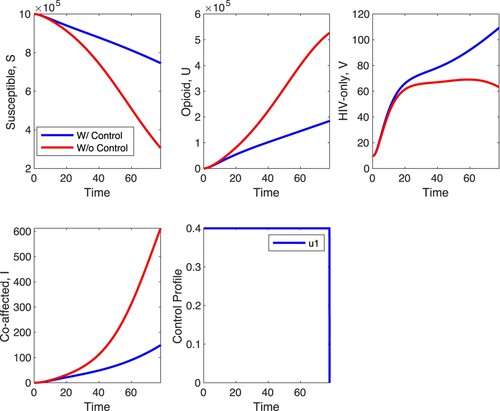
We first simulate scenario A with $u_1^{max}=0.4$. These results are shown in Figures 1 and 2. In Figure 1, ${\text{β}}_u$ is fixed at its fitted value, and in Figure 2, ${\text{β}}_u$ is fixed at 1/10 of its fitted value. The figures show that opioid treatment decreases the number of opioid cases and co-affected individuals but leads to an increase in the number of HIV cases. This last effect is quite pronounced in Figure 1. In the absence of control the HIV-infected decline to zero (this is the long-term outcome with fitted parameters) but with control the number of HIV explodes. The optimal control suggests that treatment should be applied at the maximal possible level regardless of ${\text{β}}_u$. The explosion of HIV cases in the presence of control suggests that the two diseases are in a competitive regime with the fitted parameter values; suppressing one of them with control leads to an increase in the number of cases of the other. This is the outcome regardless of ${\text{β}}_u$. In comparison to the case without any form of control, there is approximately a 3.7% decrease in the number of co-affected individuals at the end of the time horizon when strategy A is applied. When ${\text{β}}_u$ is at 1/10 of its fitted value, the difference in the susceptible, opioid, HIV and co-affected populations with and without control is more pronounced compared to the case when ${\text{β}}_u$ is at the fitted value.

Figure 1. Simulations for $u_1$-only when $u_1^{max}=0.4$ and ${\text{β}}_u=0.385676$ (fitted value).

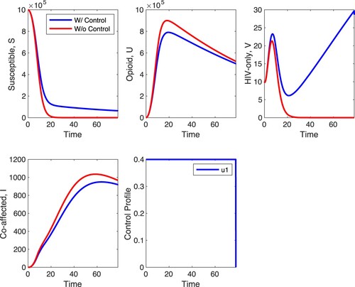
Figure 2. Simulations for $u_1$-only when $u_1^{max}=0.4$ and ${\text{β}}_u=0.1\times 0.385676$.

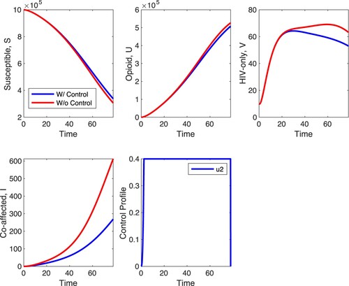
In scenario B, we apply only control measures which decrease the coefficient through which opioid-addicted individuals get HIV, namely $q_v$. Without control, the fitted value suggested that coefficient $q_v$ is much higher than one. Decreasing it with control is shown in Figures 3 and 4. Both figures are obtained with control $u_2$ being on with maximum $u_2^{max}=0.4$. In Figure 3, ${\text{β}}_u$ is at its fitted value while in Figure 4, ${\text{β}}_u$ is at 1/10 of its fitted value. From both figures we infer that the impact of this control is relatively minimal in the susceptible, opioid and HIV-only populations, but with about a 42% decrease in the number of co-affected individuals at the end of the time horizon when strategy B is applied compared to the case with no control. The control can both increase or decrease opioid cases but in Figure 4, it is clearly seen that it decreases the HIV cases and with about a 56% decrease in the number of co-affected individuals at the end of the time horizon. The control also has a significant impact on co-affected individuals in both figures. The impact of control $u_2$ on co-affected individuals is more pronounced than the impact of control $u_1$ with the fitted value of ${\text{β}}_u$. The optimal control suggests that the measures should gear up to the maximum quickly and be applied at the maximum possible value for the duration of the control.

Figure 3. Simulations for $u_2$-only when $u_2^{max}=0.4$ and ${\text{β}}_u=0.385676$ (fitted value).

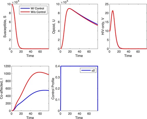
Figure 4. Simulations for $u_2$-only when $u_2^{max}=0.4$ and ${\text{β}}_u=0.1\times 0.385676$.

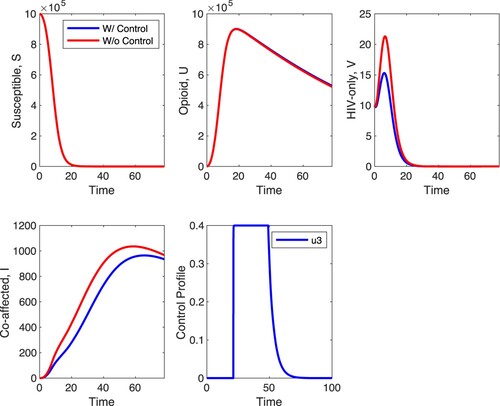
Figures 5 and 6 depict the between-host and within-host impact of control $u_3$. Control $u_3$ serves as an entry inhibitor, which decreases the infection rate of healthy T cells at the within-host level. With a maximum control of $u_3^{max}=0.4$, results of simulations shown in Figure 5 depict a decrease in the within-host infected T cells, $T_i$, and viral load $V_i$ but relatively minimal increase in healthy T cells. Unlike in Figure 3 where there is a minimal effect in the S, U and V populations with $u_2$-only, Figure 6 shows that at the between-host level, there is a minimal effect in the S and U populations when strategy C is applied with the biggest effect of the control in HIV-only infected individuals and co-affected individuals. In HIV-only individuals, the control decreases the peak of the number of infected individuals, and has a similar effect on the co-affected individuals. The control has almost no impact on opioid-only affected individuals and susceptible individuals. What is unexpected is that the optimal control is at maximal value for about 20 time units and zero for most of the remaining time suggesting that treatment is optimal with interruptions.

Figure 5. Simulations of the within-host model for $u_3$-only when $u_3^{max}=0.4$.

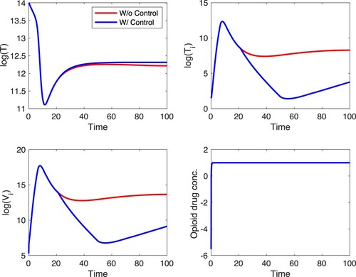
Figure 6. Simulations of the between-host model for $u_3$-only when $u_3^{max}=0.4$.

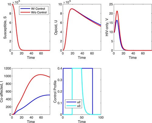
In the remaining Figures, we explore scenarios which combine several controls. In Figure 7, we explore scenario D, that is, controls $u_2$ and $u_3$ are on and the remaining controls are off. In this scenario, treatment is applied to co-affected individuals with HIV medications that prevent the fusion of HIV with target cells and control measures are applied, designed to decrease the coefficient of infection of opioid-affected individuals with HIV. Control $u_2$ is a between-host control while control $u_3$ is a within-host control. It is striking that the effect of this combined control strategy on the between host level is very similar to the effect of the within-host control $u_3$ only (see Figure 6). The main difference is in the level of co-affected individuals whose density is further decreased; there is approximately a 47% decrease in the number of co-affected individuals at the end of the time horizon when strategy D is applied compared to the case with no control. For the optimal control, control $u_2$ should be applied at maximal level within the first 80 time units. The optimal control $u_3$ is very similar as in scenario C. The optimal control $u_3$ should be applied at maximum between approximately 20 and 60 time units and then it should be at or near zero the remaining time.

Figure 7. Simulations of the between-host model when $u_2^{max}=u_3^{max}=0.4$.

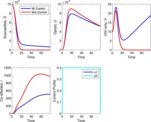
In Figure 8, we simulate scenario E. In scenario E the between-host controls $u_1$ and $u_2$ are on and the within-host controls are off. The results of these simulations are very similar to the results of simulations with scenario A. The controls increase the number of susceptible individuals and decrease the number the opioid-only affected individuals. The biggest impact of this control scenario is on HIV-only infected individuals which increase with controls while going to zero without the controls. Co-affected individuals are also very impacted by the between-host controls with their density dropping to 47% from its uncontrolled maximum relative to 3.7% when strategy A is applied, as depicted in Figure 1. The optimal controls are at the maximum value for the duration they are applied. The main difference between the results in scenario A and scenario E are in the density of co-affected individuals. Their density is significantly reduced with the controls in scenario E.

Figure 8. Simulations of the between-host model when $u_1^{max}=u_2^{max}=0.4$.

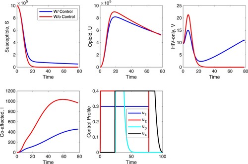
Finally, we explore scenario F in Figure 9. In scenario F, all controls are on with $u_1^{max}=0.3$ and $u_2^{max}=u_3^{max}=u_4^{max}=0.4$. The outcomes of the application of all four controls are complex. The susceptible individuals are increased. However, both the opioid-only individuals and the HIV-only individuals are impacted one way until some threshold time $t^{\ast }$ and then they are impacted the other way. In particular, the number of opioid-only individuals is decreased till time unit 70 or so and then it is increased. The number of HIV-only individuals is also decreased but until time unit 18 or so and then it is increased by the controls. The maximum of the density of the co-affected individuals is decreased maximally compared to all control scenarios we explored, with approximately a 53% decrease in the number of co-affected individuals at the end of the time horizon. The optimal control of each control is different but most controls need to be applied at maximum for some duration of time and then switched off. In particular, controls $u_1$ and $u_2$ are applied at maximum until time unit 80, and then turned off. Control $u_3$ is applied at maximum for time units between 20 and 40 and gradually turned off. Control $u_4$ is applied at maximum until time unit 90 and then gradually turned off.

Figure 9. Simulations of the between-host model when $u_1^{max}=0.3$, $u_2^{max}=u_3^{max}=u_4^{max}=0.4$.

Direct comparison of all strategies suggests that the best strategy is strategy F with all controls applied. This means that treating HIV-infected individuals and opioid-addicted individuals has to be coupled with control measures that reduce the propensity of opioid-addicted individuals to get HIV. This conclusion is further ascertained by evaluating the values of the objective functional in Equation (8(8) $\begin{array}{rl}\mathcal{J}\left(\mathbf{u}\right)& ={\int }_0^{t_f}\left[A_{1}U\right(t)+A_{2}V(t)+A_3{\int }_0^{{\tau }_f}i(\tau ,t\left)\mathrm{d}\tau \right]\mathrm{d}t\\ & +{\int }_0^{t_f}(A_4{u}_1\left(t\right)U\left(t\right)+B_1{u}_1^2(t)+B_2{u}_2^2(t\left)\right)\mathrm{d}t\\ & +{\int }_0^{{\tau }_f}\left(B_3{u}_3^2\right(\tau )+B_4{u}_4^2(\tau \left)\right)\mathrm{d}\tau ,\end{array}$(8) ) for strategies A, B, C, D, E and F, depicted in Table 1.

Table 1. Values of the objective functional for different strategies.

Strategy	A	B	C	D	E	F
Values of $\mathcal{J}$	$1.4410\times {10}^8$	$1.1189\times {10}^8$	$1.3903\times {10}^8$	$1.0022\times {10}^8$	$1.0048\times {10}^8$	$8.7781\times {10}^7$

Strategy F has the lowest value of the objective functional, followed by strategy D. Previously, we have reported that treating opioid-addicted individuals and reducing HIV infection of opioid-addicted individuals is the best strategy [25], which corresponds to strategy D. Here, we find that in terms of optimal strategies, combining the two measures in strategy D with HIV treatment is expected to reduce the number of affected individuals better.

6. Discussion

We developed a multi-scale model of HIV and opioid epidemics to get a comprehensive understanding of how these two diseases interact with each other [25,26]. The multi-scale model includes HIV and opioid dynamics at within-host and between-host scales. In this study, we apply the optimal control theory to the multi-scale model of the two diseases and evaluate the control measures adopted against HIV and opioid at both scales.

Our previous study with a single-scale model of the two epidemics suggested that the most effective control measures are preventing the opioid abuse ($u_1\left(t\right)$) and reducing the HIV risk among opioid users ($u_2\left(t\right)$). While ($u_1\left(t\right)$) and ($u_2\left(t\right)$) are the population-level control approaches, the most effective defense strategy against HIV, the anti-retro-viral therapy (ART), as it is described by CDC acts at the within-host level. We used two control measures at this scale, antiviral therapy preventing the HIV from entering target cells ($u_3\left(t\right)$) and antiviral therapy preventing the infected target cells from producing new HIV particles ($u_4\left(t\right)$). While other control strategies against HIV and opioid addiction are possible, we focus on these four as the most promising control strategies in combating the two diseases.

We formulated an optimal control problem with the objective of minimizing the number of infected, addicted and co-affected individuals as well as the cost of the control strategies. We first proved that the states of the multi-scale model are Lipschitz as a function of the controls $u_1,u_2,u_3,u_4$. Then we proved the existence and uniqueness of the optimal control strategy using Ekeland's principle.

Our numerical simulations show that when only opioid-addicted individuals are treated, the number of opioid users and the co-affected individuals decrease, but that strategy leads to an increase in the number of HIV-infected individuals. This outcome is unexpected, since in the absence of control the number of HIV-infected individuals drops to zero, but with this control strategy the number of HIV-infected individuals increases. This might be due to the fact that the two diseases, HIV and opioid are in competition, suppressing one leads to increase in the other. When we reduced the risk of an opioid user being infected with HIV, this second control strategy impact on the opioid and HIV-only populations is minimal, but its impact on the co-affected populations is significant. The effect of the control $u_2$ on the opioid population is not clear; depending on the addiction rate, ${\text{β}}_u$, we observe both an increase and decrease in the number of opioid users. In comparing the two population levels controls, $u_1$ and $u_2$, we notice that $u_2$ has more pronounced effect on the co-affected population.

When co-affected individuals receive entry inhibitor antiviral medication, we observe a decrease in both the co-affected and HIV-only populations. Antiviral treatment of co-affected individuals, in particular, lowers the peak number of HIV-infected population, which is an important public health goal. If the antiviral therapy is combined with reducing the risk of HIV in opioid users, we again observe a decrease in both the co-affected and HIV-only populations.

The maximal reduction in co-affected individuals is observed when multiple controls are active, that is in the cases when $u_2$ and $u_3$ are simultaneously active or when $u_1$ and $u_2$ are simultaneously active. When $u_2$ and $u_3$ are simultaneously active, the HIV-only population declines to zero with or without the controls but the opioid-addicted population experiences no decline. When $u_1$ and $u_2$ are simultaneously active, the opioid population experiences decline but the HIV-only population increases after a period of decrease. These two opposing effects are best combined when all four controls are active. With all four controls active, the co-affected population experiences maximum decline, the opioid-addicted population declines and the ultimate increase in the HIV-only population is reduced. Thus we suggest that our best strategy among the ones investigated is the strategy where all four controls are active. In other words, from a public heath perspective, it is best to treat opioid-addicted individuals, treat co-affected individuals with ART, and prevent opioid addicted individuals from contracting HIV.

Disclosure statement

No potential conflict of interest was reported by the author(s).

Additional information

Funding

Maia Martcheva acknowledges partial support from National Science Foundation (NSF) [grant number DMS-1951595]. Necibe Tuncer acknowledges partial support from National Science Foundation (NSF) [grant number DMS-195626].

References

- National Institute of Drug Abuse (NIH). Overdose death rates; 2022 Jan. Available from: https://nida.nih.gov/research-topics/trends statistics/overdose-death-rates.
- U.S. Department of Health and Human Services. What is the U.S. opioid epidemic? 2019. Available from: https://www.hhs.gov/opioids/about-the-epidemic/index.html.
- National Institute for Drug Abuse (NIH). Drug use and viral infections (HIV, hepatitis), drug facts. Available from: https://www.drugabuse.gov/publications/drugfacts/drug-use-viral-infections-hiv-hepatitis.
- E. White, C. Comiskey. Heroin epidemics, treatment and ODE modelling. Math Biosci. 2007;208:312–324. doi: 10.1016/j.mbs.2006.10.008
- F. Nyabadza, S.D. Hove-Musekwa. From heroin epidemics to methamphetamine epidemics: modelling substance abuse in a South African province. Math Biosci. 2010;225:132–140. doi: 10.1016/j.mbs.2010.03.002
- G.P. Samanta. Dynamic behaviour for a nonautonomous heroin epidemic model with time delay. J Appl Math Comput. 2011;35:161–178. doi: 10.1007/s12190-009-0349-z
- B. Fang, X. Li, M. Martcheva, et al. Global stability for a heroin model with two distributed delays. Discrete Contin Dyn Syst Ser B. 2014;19:715–733.
- G. Huang, A. Liu. A note on global stability for a heroin epidemic model with distributed delay. Appl Math Lett. 2013;26:687–691. doi: 10.1016/j.aml.2013.01.010
- J. Liu, T. Zhang. Global behaviour of a heroin epidemic model with distributed delays. Appl Math Lett. 2011;24:1685–1692. doi: 10.1016/j.aml.2011.04.019
- B. Fang, X. Li, M. Martcheva, et al. Global stability for a heroin model with age-dependent susceptibility. J Syst Sci Complex. 2015;28:1243–1257. doi: 10.1007/s11424-015-3243-9
- B. Fang, X.-Z. Li, M. Martcheva, et al. Global asymptotic properties of a heroin epidemic model with treat-age. Appl Math Comput. 2015;263:315–331.
- J. Wang, J. Wang, T. Kuniya. Analysis of an age-structured multi-group heroin epidemic model. Appl Math Comput. 2019;347:78–100.
- J. Yang, X. Li, F. Zhang. Global dynamics of a heroin epidemic model with age structure and nonlinear incidence. Int J Biomath. 2016;9:Article ID 1650033, 20.
- N.A. Battista, L.B. Pearcy, W.C. Strickland. Modeling the prescription opioid epidemic. Bull Math Biol. 2019;81:2258–2289. doi: 10.1007/s11538-019-00605-0
- S. Cole, S. Wirkus. Modeling the dynamics of heroin and illicit opioid use disorder, treatment, and recovery. Bull Math Biol. 2022;84:Article ID 48, 49. doi: 10.1007/s11538-022-01002-w
- T. Phillips, S. Lenhart, W.C. Strickland. A data-driven mathematical model of the heroin and fentanyl epidemic in Tennessee. Bull Math Biol. 2021;83:Article ID 97, 27. doi: 10.1007/s11538-021-00925-0
- S.R. Rivas, A.C. Tessner, E.E. Goldwyn. Calculating prescription rates and addiction probabilities for the four most commonly prescribed opioids and evaluating their impact on addiction using compartment modelling. Math Med Biol. 2021;38:202–217. doi: 10.1093/imammb/dqab001
- G.K. Befekadu, Q. Zhu. Optimal control of diffusion processes pertaining to an opioid epidemic dynamical model with random perturbations. J Math Biol. 2019;78:1425–1438. doi: 10.1007/s00285-018-1314-y
- A. Khan, G. Zaman, R. Ullah, et al. Optimal control strategies for a heroin epidemic model with age-dependent susceptibility and recovery-age. AIMS Math. 2021;6:1377–1394. doi: 10.3934/math.2021086
- P.K. Roy. Mathematical models for therapeutic approaches to control HIV disease transmission. Singapore: Springer; 2015.Industrial and Applied Mathematics,
- W.-Y. Tan, H. Wu. Deterministic and stochastic models of AIDS epidemics and HIV infections with intervention. Hackensack, NJ: World Scientific Publishing Co. Pte. Ltd.; 2005.
- U. Habibah, R.A. Sari. Optimal control analysis of HIV/AIDS epidemic model with an antiretroviral treatment. Aust J Math Anal Appl. 2020;17:Article ID 16, 11.
- H. Zhao, P. Wu, S. Ruan. Dynamic analysis and optimal control of a three-age-class HIV/AIDS epidemic model in China. Discrete Contin Dyn Syst Ser B. 2020;25:3491–3521.
- X.-C. Duan, X.-Z. Li, M. Martcheva. Coinfection dynamics of heroin transmission and hiv infection in a single population. J Biol Dyn. 2020;14:116–142. doi: 10.1080/17513758.2020.1726516
- C. Gupta, N. Tuncer, M. Martcheva. Immuno-epidemiological co-affection model of hiv infection and opioid addiction. Math Biosci Eng. 2022;19:3636–3672. doi: 10.3934/mbe.2022168
- C. Gupta, N. Tuncer, M. Martcheva. A network immuno-epidemiological model of hiv and opioid epidemics. Math Biosci Eng. 2023;20:4040–4068. doi: 10.3934/mbe.2023189
- A.N. Timsina, N. Tuncer. Dynamics and optimal control of hiv infection and opioid addiction. In: Tuncer N, Martcheva M, Childs L, Prosper O, editors. Computational and mathematical population dynamics. New Jersey, Boca Raton: World Scientific; 2023 (in press), Chapter 2.
- E. Numfor, S. Bhattacharya, S. Lenhart, et al. Optimal control in coupled within-host and between-host models. Math Model Nat Phenom. 2014;9:171–203. doi: 10.1051/mmnp/20149411
- E. Numfor, S. Bhattacharya, M. Martcheva, et al. Optimal control in multi-group coupled within-host and between-host models. In: Proceedings of the Tenth MSU Conference on Differential Equations and Computational Simulations; San Marcos, TX: Texas State Univ.–San Marcos, Dept. Math.; 2016. p. 87–117. (Electronic Journal of Differential Equations Conference; 23).
- P. Wu, Z. He, A. Khan. Dynamical analysis and optimal control of an age-since infection HIV model at individuals and population levels. Appl Math Model. 2022;106:325–342. doi: 10.1016/j.apm.2022.02.008
- I. Ekeland. On the variational principle. J Math Anal Appl. 1974;47:324–353. doi: 10.1016/0022-247X(74)90025-0
- M. Nowak, R. May. Virus dynamics: mathematical principles of immunology and virology. New York, USA: Oxford University Press; 2000.
- A.S. Perelson, P.W. Nelson. Mathematical analysis of HIV-I: dynamics in vivo. SIAM Rev. 1999;41:3–44. doi: 10.1137/S0036144598335107
- A. Lange, N. Ferguson. Antigenic diversity, transmission mechanisms, and the evolution of pathogens. PLoS Comput Biol. 2009;5(10):e1000536.
- M. Martcheva. An introduction to mathematical epidemiology. New York: Springer; 2015.Vol. 61 of Texts in Applied Mathematics,
- M.A. Gilchrist, D. Coombs. Evolution of virulence: interdependence, constraints, and selection using nested models. Theor Popul Biol. 2006;69:145–153. doi: 10.1016/j.tpb.2005.07.002
- E. Numfor, S. Bhattacharya, M. Martcheva, et al. Optimal control applied in coupled within-host and between-host models. Math Model Nat Phenom. 2014;9:171–203. doi: 10.1051/mmnp/20149411
- E. Numfor, S. Bhattacharya, M. Martcheva, et al. Optimal control in multi-group coupled within-host and between-host models. Electron J Differ Equ Conf. 2016;23:87–117.
- M. Shen, Y. Xiao, L. Rong, et al. Conflict and accord of optimal treatment strategies for HIV infection within and between hosts. Math Biosci. 2019;309:107–117. doi: 10.1016/j.mbs.2019.01.007
- Centers for Disease Control and Prevention. Effectiveness of prevention strategies to reduce the risk of acquiring or transmitting hiv. Available from: https://www.cdc.gov/hiv/risk/estimates/preventionstrategies.html.
- S. Lenhart, J.T. Workman. Optimal control applied to biological models. Boca Raton, FL: Chapman & Hall/CRC; 2007.Chapman & Hall/CRC Mathematical and Computational Biology Series,
- V. Barbu. Mathematical methods in optimization of differential systems. Dordrecht: Kluwer Academic Publishers; 1994.
- E. Numfor. Optimal treatment in a multi-strain within-host model of hiv with age structure. J Math Anal Appl. 2019;480:Article ID 123410. doi: 10.1016/j.jmaa.2019.123410
- S. Lenhart, J.T. Workman. Optimal control applied to biological models. Baco Raton: Chapman and Hall; 2007.