3D reconstruction of partial foot scans using different state of the art neural network approaches

Abstract

As online shopping continues to grow in popularity, shoes are increasingly being purchased without being physically tried on. This has resulted in a significant surge in returns, causing both financial and environmental consequences. To tackle this issue, several systems are available to measure foot dimensions accurately either in-store or at home. By obtaining precise foot measurements, individuals can determine their ideal shoe size and prevent unnecessary returns. In order to make such a system as simple as possible for the user, only a single image should be sufficient to measure the foot. To make this possible, point clouds from one side of the foot, which are generated by taking a depth image, are to be used. Since these point clouds represent only one side of the foot, the other side has to be generated. For this purpose, different existing state of the art networks were tested and compared to determine which architecture is best suited for this task. After implementing, re-training on our own dataset and testing the different architectures, it can be concluded that the point/transormer-based network SnowflakeNet is the most efficient to be used for our task.

Keywords:

• Foot measurement
• shape completion
• shape reconstruction
• GAN
• neural network
• machine learning
• CNN

1. Introduction

Due to the rise of online shopping for clothing and shoes, especially during the Corona pandemic, trying on shoes in a physical store to determine the correct size is no longer attractive. As a result, people often order multiple pairs of shoes in different sizes and return those that do not fit, causing significant financial and environmental damage. In Germany alone, approximately 286 million items ‘(Asdecker, 2019)’ are returned, with 21.4% (Brandt, 2023) being shoes that are typically returned because they are either too big or too small. With an average loss of 15.18€per return (Asdecker, 2019), this results in an annual financial loss of €4.34 billion and 242,814 tons of CO2 emissions (Asdecker, 2022). To address this issue, there is a need for a simple system that can accurately measure feet from anywhere and determine the appropriate shoe size, thereby reducing the number of returns. While there are numerous systems and methods available, many now rely on computer vision rather than traditional measuring tools, using photogrammetry from 2D images, 3D point clouds, or image processing with 2D RGB images. In addition to the growing online market, the availability of 3D sensors to the public has increased significantly. Several smartphones (e.g. iPhone 14 Pro) have Time of Flight sensors built into their main camera. The problem is that many recorded point clouds are incomplete due to several reasons as reflections, resolution or many others. To recover this imperfect data, shape completion is used.

2. Related work

The objective of Point Cloud Completion is to recover a complete shape from incomplete data. For example, this task is used to develop various applications in the field of autonomous driving (Monica & Campbell, n.d.), robotics (Engel et al., 2014; Mur-Artal et al., n.d.), fabrication or 3D modelling (Hu & Kneip, 2021). In the beginning, this task was approached along the example of 2D completion tasks, as can be seen in (Dai et al., 2016; Liu et al., 2019; Stutz & Geiger, n.d.). In that case voxelization and 3D convolution were used. With voxelization, it was tried to create a grid similar to the one that exists in 2D images. However, the disadvantage of these approaches is that they have very high computational costs. The major success in the area of shape completion came with networks such as PointNet (Qi et al., 2016) or Point Completion Network (PCN) (Yuan et al., 2018), which process 3D coordinates directly. Since the first successful implementations of Generative Adversarial Networks (GANs) in the field of 3D data generation (W. Wang et al., 2017; Wu et al., 2016), nowadays they have become an important tool in the field of shape completion.

Another successful current method is Transformer Networks. Powered by its attention mechanism and outstanding capacity to record long-range interactions, Transformer-based approaches have made a notable transition from Convolutional Neural Networks to the computer vision community in recent years. Researchers have expanded the use of Transformers to jobs involving point cloud analysis in response to this trend. The effective use of Transformer topologies for point cloud decoding has been made possible by notable innovations like Pointformer (X. Pan et al., 2021), SnowflakeNet (Xiang et al., 2021), and PointTr (Yu et al., 2021), which guarantee the preservation of delicate geometrical features.

3. Methods

In the following chapter, we discuss the networks used for shape completion of feet point clouds. The networks studied were originally developed for application to the ShapeNet (Chang et al., 2015), KITTI (Geiger et al., 2013) or Completion3D (Lyne Tchapmi et al., 2019) datasets. Since they give excellent results there, this study investigated whether it is also possible to reconstruct incomplete feet using these architectures. When selecting the networks, emphasis was placed on using state of the art networks with different architectures. Current Point Cloud Completion networks can be divided into the following categories according to Fei et al. (2022):

• GAN-based Methods

• Convolution-based Methods

• Point-based Methods

• Graph-based Methods

• View-based Methods

• Variational Auto-Encoder (VAE)-based Methods

• Transformer-based Methods

Five architectures were investigated in this research, namely Shape Inversion GAN (GAN-based), PoinTr (Point-/Transformer-based), VRCNet (VAE-based), SnowflakeNet (Point-/Transformer-based) and PointAttN (Point-based).

3.1. Shape Inversion GAN

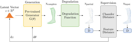
This study explores the use of a well-trained GAN as a prior for shape completion, specifically for handling partial shapes of various types and generalizing to unseen shapes. Shape Inversion GAN is trained on 3D shapes and can generate a complete shape from a latent vector. GAN inversion is used to find the best latent vector that reconstructs a given shape. The generator is fine-tuned during inversion as seen in recent approaches (Bau et al., 2019; X. Pan et al., 2020), and the distance is computed at the observation space. A degradation function is used to transform a complete shape into a partial form (Zhang et al., 2021).

Figure 1 shows the architecture of Shape Inversion. A vector z is used by the generator to produce a complete shape. During degradation, this shape is then converted to a partial shape. Finally, the parameter θ of G is fine-tuned by Shape Inversion to obtain the best possible reconstruction (Zhang et al., 2021).

Figure 1. Operating principle of Shape Inversion GAN for shape completion (Zhang et al., 2021).

3.2. PoinTr

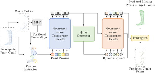
The PoinTr network, shown in Figure 2, solves the point cloud completion problem along the lines of a set-to-set translation task. The network is trained with the point proxies of the partial point clouds and produces the point proxies of the missing parts to generate a complete geometry. The encoder-decoder architecture used employs L_E and L_D multi-head self-attention layers. To enhance the decoder’s ability to handle missing parts of various types of objects, dynamic query embeddings are used for predicting point proxies (Yu et al., 2021).

Figure 2. Operating principle of PoinTr for shape completion (Yu et al., 2021).

3.3. VRCNet

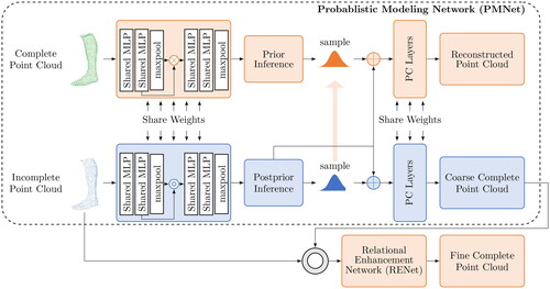
The VAE-based method VRCNet uses a dual-path architecture, as can be seen in Figure 3. This involves a construction and a reconstruction path. The construction path is only used for training. The reconstruction path is used to create a coarse complete point cloud. Afterwards, the coarse point cloud is densified and finer details are recovered. This last step is done with the help of a RENet. The network was originally trained on the MVP dataset, which consists of 100,000 high-resolution partial and complete point clouds. Compared to other methods that use virtual cameras to render images with relatively low resolution (160 × 120), this method uses images with a resolution of 1600 × 1200 (L. Pan et al., 2021).

Figure 3. Operating principle of VRCNet for shape completion (L. Pan et al., 2021).

3.4. SnowflakeNet

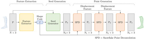
SnowflakeNet is a transformer-based network for point cloud completion. Figure 4 shows the design of the network. As can be seen there, this network consists of a feature extractor, a seed generator and a point generator. The feature extractor generates a shape code which contains the local structural details as well as the global context of the object. Subsequently, a sparse point cloud is generated in the seed generator based on this information. This cloud is already complete, even if it is not particularly dense. Finally, the point generator, which processes the information from the shape code and the sparse point cloud, generates a fine grained point cloud using Snowflake Point Deconvoluton (SPD). This SPD has the function of increasing the number of points for the final point cloud. For this purpose, each parent point is split into several child points, which are created by copying and then varying the parent points (Xiang et al., 2021).

Figure 4. Operating principle of SnowflakeNet for shape completion (Xiang et al., 2021).

3.5. PointAttN

Figure 5 showcases the general structure of PointAttN, which is suggested. The structure utilizes the widely used encoder-decoder design for accomplishing point cloud completion. Similar to SnowflakeNet, the framework consists of three main modules: a shape feature encoder for feature extraction, a seed generator module, and a point generator module that work together to generate the complete shape in a coarse-to-fine manner (J. Wang et al., 2022). The difference, however, is that self-feature augment (SFA) is used in the point generator. SFA is a method for predicting the complete point cloud by utilizing self-attention to establish spatial relationships among points. It reveals detailed geometry of 3D shapes and can also enhance feature representation ability by capturing global information (J. Wang et al., 2022).

Figure 5. Operating principle of PointAttN for shape completion (J. Wang et al., 2022).

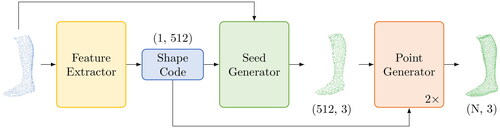
Figure 6. Baseline feet created from all feet of the training dataset.

3.6. Baseline model

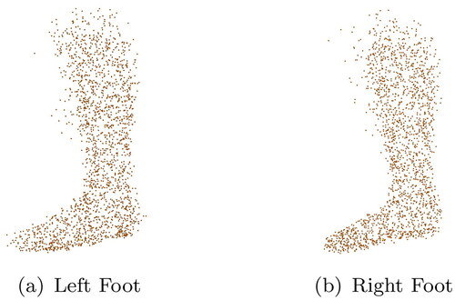
Simultaneously with the networks, a baseline model was created to evaluate how far a simple approach can get and how much better the neural networks are in direct comparison. The baseline model was created by overlaying all normalized feet from the training dataset to get a single large point cloud. This step was carried out for all left and all right feet. By deleting random points, the number of points is then reduced to 2048. We then always used the point cloud of either the left or right foot as the reconstruction result to see if an ‘average foot’ might be good enough as a reconstruction. The left and right base foot generated in this process can be seen in Figure 6.

3.7. Datasets

Nowadays, different datasets are used for the task of point cloud completion. These can essentially be broken down into real-world scans and artificially generated data. The KITTI dataset, for example, contains real-world LiDAR scans and RGB images of public traffic scenes. The remaining well-known large datasets, which are synthetically generated datasets, are for example PCN, ShapeNet, Completion3D (C3D) or Multi-View Partial Point Cloud (MVP). These all contain between 8 and 55 classes of diverse objects such as lamps, aeroplanes, cars, etc.

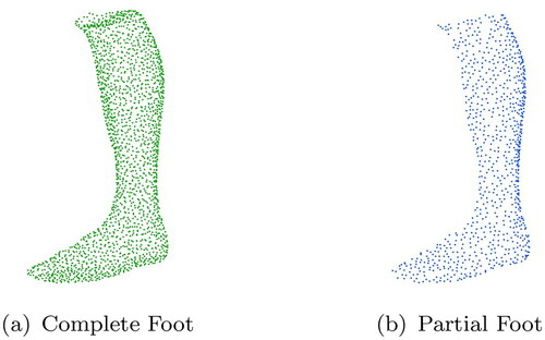
The dataset used in this study is from corpus.e AG in Stuttgart, Germany, and includes 1000 high-resolution foot scans, 500 of them being male and 500 female. Each file represents a foot scan, which includes the foot up to the knee. The original data, which is in .stl format, was converted to point cloud using the Open3D (Zhou et al., 2018) sample_points_poisson_disk method. The number of points for the complete point clouds is set to 2048 points. Furthermore, all point clouds are normalized to a range of [−0.5, 0.5]. Using the Open3D hidden point removal method, profile views are generated from the complete point clouds, leaving only half a point cloud of each foot as can be seen in Figure 7(b). This procedure is intended to simulate the recording of the foot with a 3D camera from one perspective. The native data format was chosen for each network. For Shape Inversion it is .ply, for PoinTr, SnowflakeNet and PointAttN .pcd and for VRCNet .h5 format. The formats were kept in order not to change the architecture of the networks. Nevertheless, in the end they are all coordinate conversions that contain the same information. An example scan is shown in Figure 7(a). The corpus.e dataset was divided into training (696 scans), validation (157 scans) and test (153 scans) data set.

Figure 7. Example point cloud from the training dataset.

For all networks, the respective pre-trained weights of the authors were used as the starting point for our training. Since the objects in all datasets used to create these weights are similar (e.g. cars, aeroplanes, tables, etc.) and since no people or feet are included, we considered the starting points of each network to be the same. In the next step, the networks were re-trained using our feet dataset.

In the experiments for this publication, only the profile view of the foot was used for training. This view was selected because it shows the length of the foot, which is one of the most important factors for a shoe fit. In a future step, other views of the foot will be used for training to make the network more robust to different points of view. Since this study only investigates whether a reconstruction from a single depth image is generally possible, errors that would occur when using a real depth camera (e.g. flying pixels, multi path errors etc.) are not shown. Also, background and floor, which can be seen in a real depth image, are not included in this simulation.

Table 1. Hyperparameters for Shape Inversion (Zhang et al., 2021), PoinTr (Yu et al., 2021), VRCNet (L. Pan et al., 2021), SnowflakeNet (Xiang et al., 2021) and PointAttN (J. Wang et al., 2022).

	Shape Inversion	PoinTr	VRCNet	SnowflakeNet	PointAttN
Learning rate	0.0001	0.0005	0.0001	0.001	0.0001
Epochs	2000	300	300	400	300
Batch size	2	4	13	1	8
Loss function	CD	CD L1	CD	CD L1	CD
Optimizer	Adam	Adam	Adam	Adam	Adam

3.8. Hyperparameters

The hyperparameters for the networks were chosen as determined by the authors of the respective networks, as can be seen in Table 1. Only the batch size was changed depending on the hardware utilization. If there was no number of epochs specified, the number of epochs was adjusted until the result converged to a value. The number of epochs was then chosen accordingly.

3.9. Implementation details

The networks were implemented on a Linux system running four Nvidia Titan RTX GPUs. When training the individual networks, the pre-trained weigths provided by the authors were used. None of the datasets used by the authors contain feet or people and all of them generally consist of very similar objects. Therefore, these pre-trained networks used as starting points for our training are considered equivalent.

3.10. Metrics

Four metrics were used to evaluate the effectiveness of each network. The tested networks all use the Chamfer Distance. However, since this metric also has its limitations, and we did not want to rely on just one value, we decided to use four metrics for the evaluation. These are the Chamfer Distance (CD), the F-Score, the Earth Mover’s Distance (EMD) and the Hausdorff Distance. Each of these metrics has advantages and disadvantages that we will briefly discuss below.

3.10.1. Chamfer Distance (CD)

The Chamfer Distance (Fan, Su, & Guibas, n.d.) is a widely used metric for evaluating the equality of point clouds, which has been used in numerous other works such as (Huang et al., 2020; Lyne Tchapmi et al., 2019; Xie et al., 2020; Yuan et al., 2018). The metric is calculated by adding the squared distances between two point clouds’ nearest neighbour correspondences. The CD gets calculated as follows: (1) $$d_{\mathit{\text{CD}}}(X,Y)={\displaystyle \sum }_{x\in X}\underset{y\in Y}{\text{min}}{‖x-y‖}_2^2+{\displaystyle \sum }_{y\in Y}\underset{x\in X}{\text{min}}{‖x-y‖}_2^2$$(1)

One of the main advantages is its simplicity. The Chamfer Distance is easy to calculate and understand. The lower the Chamfer Distance, the better the result. Additionally, it is sensitive enough to detect small differences between point clouds, making it useful for object recognition and model evaluation. Moreover, it is a fast metric, allowing it to be used for large point clouds. Anyways, the Chamfer Distance also has some limitations. It may perform poorly when dealing with unevenly distributed point clouds. If, for example, a point cloud has an area with high point density and another area with low point density, the Chamfer Distance may not accurately represent the similarity between the two point clouds. Furthermore, it is susceptible to outliers and noise in the point clouds, which may lead to errors in the evaluation.

3.10.2. F-Score

The F-Score, introduced by Tatarchenko et al. (2015), is another commonly used metric for evaluating point clouds. It is calculated as follows: (2) $$F-\mathit{\text{Score}}(d)=\frac{2\cdot P(d)\cdot R(d)}{P(d)+R(d)}$$(2) (3) $$P(d)=\frac{1}{\left|X\right|}{\displaystyle \sum }_{r\in Y}\left[\underset{t\in Y}{\text{min}}‖t-r‖<d\right]$$(3) (4) $$R(d)=\frac{1}{\left|Y\right|}{\displaystyle \sum }_{t\in Y}\left[\underset{r\in X}{\text{min}}‖\left|t-r\right|‖<d\right]$$(4) where P(d) represents the precision and R(d) the recall for a distance threshold d.

The higher the F-Score, the better the result. It takes into account both precision and recall, providing a balanced evaluation of the model’s performance. Additionally it is sensitive to both false positives and false negatives, making it suitable for evaluating the accuracy of object detection and segmentation in point clouds. However the F-Score is dependent on a threshold value d, which can affect its results, and different threshold values can lead to different F-Scores, making it difficult to compare results across studies. Finally, the F-Score may not capture all aspects of the model’s performance, such as its ability to handle noise, occlusions, or complex object geometries.

3.10.3. Earth Mover’s Distance (EMD)

The Earth Mover’s Distance (Fan et al., n.d.) is calculated as follows: (5) $$\mathit{\text{EMD}}(X,Y)=\underset{\gamma \in \Gamma (X,Y)}{\text{min}}{\displaystyle \sum }_{(x,y)\in \gamma }{‖x-y‖}_2$$(5)

To interpret the result of this calculation, a low EMD means a better result. EMD has several advantages, including its capability to capture global structural information, robustness to small deformations, and the ability to handle variable point densities. Nevertheless, there are also some disadvantages associated with EMD, such as its computational complexity and sensitivity to outliers or noise in the point clouds. Additionally, it may not be suitable for fine-grained analysis or applications where small differences between point clouds are important, as it tends to emphasize larger differences. Overall, the EMD is a useful metric for point cloud evaluation, especially for tasks where global structural information is important, but its limitations should also be taken into consideration.

3.10.4. Hausdorff Distance

The Hausdorff Distance is a commonly used metric for point cloud evaluation and is calculated as follows: (6) $$H(X,Y)=\text{max}\left(\underset{x\in X}{\text{sup\hspace{0.33em}}}\underset{y\in Y}{\text{inf}}\left|x-y\right|,\underset{y\in Y}{\text{sup}}\underset{x\in X}{\text{inf}}\left|x-y\right|\right)$$(6)

A low result in the Hausdorff Distance calculation indicates a good reconstruction result. One of its main advantages is its ability to capture fine-grained differences between point clouds, making it well-suited for tasks where small differences matter. Additionally, the Hausdorff Distance is easy to compute and has a low computational complexity. However, one major limitation is that it can be sensitive to outliers, meaning that a few outlying points can greatly affect the distance between two point clouds. This can lead to misleading results in some cases. Additionally, the Hausdorff Distance does not provide information about the distribution of distances between points in the two point clouds. Overall, the Hausdorff Distance is a useful metric for point cloud evaluation, particularly for tasks where small differences between point clouds are important. However, its sensitivity to outliers should be taken into consideration.

3.10.5. Visual inspection

In addition to the quantitative values, a qualitative evaluation of the reconstructed point clouds compared to the ground truth (GT) is performed. Looking only at the calculated values, they can be good or bad for several reasons, which are different for each of the different metrics. From the values, however, it is not possible to determine, for example, that the value is bad because the point cloud contains a lot of noise or whether the reconstruction is generally completely wrong. For this reason, we also perform an visual inspection.

4. Results

After all networks were trained with the dataset described in chapter 3.7, the generated point clouds were evaluated using the metrics defined in chapter 3.10. The results for each of the tested networks are described in this section.

4.1. Quantitative results

The quantitative results for all metrics used for evaluation of the point cloud reconstruction for all networks tested are shown in Table 2.

Table 2. Quantitative results for all networks.

Metric		Baseline model	Shape Inversion	PoinTr	VRCNet	SnowflakeNet	PointAttN
Chamfer Distance	↓	0.0561	0.0336	0.0242	0.0370	0.0169	0.0352
Earth Mover’s Distance	↓	100.16	46.502	44.189	138.22	34.759	88.793
Hausdorff Distance	↓	0.2554	0.0657	0.0627	0.1388	0.0284	0.1163
F-Score	↑	0.2610	0.3360	0.4735	0.3615	0.6768	0.4693

Looking at the results of our baseline model, we can clearly see that the results in almost all metrics are inferior to those of the much more complex neural networks. The Chamfer Distance in particular, with a value of 0.0561, is almost 3.3 times worse than our best result of 0.0169 from SnowflakeNet. Only the VRCNet can be beaten by the baseline model in the EMD. This is probably due to the fact that VRCNet follows a similar approach to the one we used for our baseline model. A foot is created, which is then used as output for all reconstructions. As both point clouds have a relatively large number of outliers, the EMD, which reacts sensitively to this, is poor in both approaches.

When examining the quantitative results for Shape Inversion it becomes evident that the obtained scores fall within the mid-range when compared to other mesh reconstruction approaches. Notably, the F-Score stands out as relatively low. This observation suggests that interpreting the data from this model presents challenges, which may be attributed to the limited size of the training dataset.

The results of PoinTr are quite close to those of SnowflakeNet and indicate a good reconstruction. Only Hausdorff Distance’s performance is noticeably worse, however, the values are still on a good level. The score could be due to outliers in the point cloud, to which the Hausdorff Distance reacts very sensitively.

In contrast, the quantitative results for VRNet indicate poor performance across various metrics, positioning it as the least favourable option among the evaluated methods. Especially the Hausdorff Distance is extremely poor, which is probably due to the fact that the point cloud has some significant outliers, as shown in Figure 8. Also, the point cloud contains a lot of noise, which leads to poor EMD results.

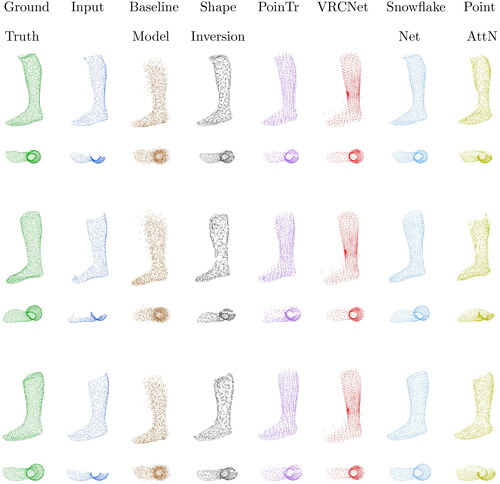
Figure 8. Qualitative results of three point cloud completions from the different networks. Each row shows a different foot from the corpus.e dataset from two different views. The first column (ground truth (GT)) shows the best possible result of the reconstruction. The second column (input) displays what the network gets as a starting point for the reconstruction. The third column shows the baseline model, which represents an average foot. The following columns show the reconstructions of the different networks from the respective input.

The metrics results of SnowflakeNet show how excellent the reconstruction in this experiment is. The network outperforms all other networks and is clearly ahead in all tested metrics. Especially the Chamfer Distance shows a very good value with 0.0169. The EMD is also extremely promising at 34.759. These excellent results might be due to the model’s excellent generalization, which should also produce good results for geometries not present in the initially used PCN dataset. Another feature that could give SnowflakeNet an advantage over the other networks is the use of skip-transformers. Compared to other methods, the spatial relationship of the point cloud points is observed over different stages of decoding. In this way, a spatial relationship between the points can be established over various steps of the decoding process so that the position of the points can be continuously refined. The skip-transformer therefore learns the shape context and the local spatial relationships of the points in each step. This enables the network to accurately capture the structural features of the object and thus generate a better shape of the point cloud with smoother surfaces as well as sharp edges.

Considering the metrics calculated for PointAttN, the results are as expected in the lower midfield. The relatively high value for the Hausdorff Distance at 0.1163 indicates, as confirmed by the Point Cloud, that a lot of outliers are present. These can be seen particularly on the underside of the foot in Figure 8.

4.2. Qualitative results

The qualitative results of the point cloud reconstruction for all networks tested are shown in Figure 8.

If you look at the point clouds of the baseline model, it can be seen that the point cloud has a relatively large number of outliers. Among other factors, these lead to a high EMD. In general, compared to the results of the neural networks, it can be said that the point cloud does not fit the ground truth as precisely, but delivers relatively good results for the simplicity of the approach.

When analysing the qualitative results of the Shape Inversion GAN it is clear that accurate reconstructions of realistic foot forms have been made for all three cases, matching the ground truth (GT). Nevertheless, an observable characteristic is the relatively narrow width of the feet generated by the network, deviating from the authentic model’s proportions.

In the case of the qualitative assessment of PoinTr, a realistic reconstruction of the missing side of the foot is also evident. However, it is noticeable that the generated point cloud has a significant amount of noise. This is especially noticeable in the second foot in Figure 8. Also, the density of the point clouds from the top view seems very leaky, since the reconstructed points are located almost exactly below each other.

Looking at the point clouds for the VRCNet, it is noticeable that the point clouds for each foot look identical. The coordinates for each point of the point clouds differ only after the fourth decimal place. Thus, the network supposedly always generates the same foot. In addition, both sides of the foot look almost symmetrical.

The point clouds generated by SnowflakeNet look extremely similar to the GT. There is no noise and the geometry of the foot is almost perfectly restored. The generated feet are only slightly narrower than the GT, which is almost unnoticeable without aligning the point clouds. In general, the performance of SnowflakeNet in these qualitative assessments is excellent.

The last network, PointAttN, shows point clouds that resemble a foot, but it is clear that the generated side is significantly less dense. Additionally, the reconstructed geometry looks like a foot but is not very accurate in comparison to the GT. The shape of the reconstructed side is entirely wrong. Also, the reconstruction shows a considerable amount of noise.

4.3. Summary

Figure 9 once again shows all the results of the evaluation in graphical form. In direct comparison with all networks, it is clearly evident that SnowfakeNet performs best in all metrics examined and thus performs the task of reconstructing incomplete foot scans best. The second best performing network is PoinTr. All metrics are relatively close to those of SnowflakeNet, except for the Hausdorff Distance. Apart from the F-Score, Shape Inversion also delivers good results. PointAttN performs in the midfield for all metrics, but the visual inspection shows clear deficiencies regarding the overall shape of the foot.

Figure 9. Results of all metrics for each of the networks tested.

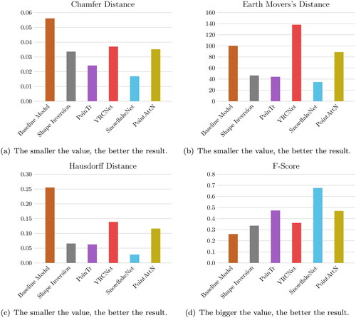
Also VRCNet, does not deliver convincing results in the foot reconstruction, both in the metrics and in the qualitative examination of the point clouds, which all look the same. The baseline model performs the worst, but this was to be expected due to the simplicity of the approach. Nevertheless, it is interesting to see how far you can get with such an approach.

5. Conclusion

This study was conducted to determine which of the state of the art networks for geometry reconstruction of incomplete point clouds performed best for the single view foot reconstruction use case. This approach is intended to replace costly scanning procedures that require multiple views of the foot. By requiring only a single depth image of the foot, which can be taken by almost anyone with a current smartphone, 3D measurement can be made accessible to the general public.

For this purpose, different network architectures were implemented and tested. For all networks, the pre-trained weights provided by the authors were used, which were generated by training with classical reconstruction datasets such as ShapeNet. These datasets contain objects such as lamps, tables, aeroplanes, etc. The networks were then re-trained and tested using our own dataset of foot scans. In the course of this investigation, it was found that the point/transformer-based approach SnowflakeNet worked most effectively and produced the best quality reconstructions from the half-point clouds.

Although this approach has a very high potential, there are also limitations. One point that could further improve the results would be to increase the size of the data set. Another limitation of the current approach is the high artificiality of the data. A consumer grade 3D sensor has significantly larger errors in the measurement than the data set acquired under laboratory conditions that we use here. Also, background and ground are already removed. Furthermore, we only used depth images from one point of view in this study. More views in the training data could significantly improve the robustness of the system. In addition, this method can probably not be applied in the field of medical foot measurement, since the reconstructed foot is only an estimate of reality. However, this estimation is perfectly sufficient for a normal selection of the shoe size.

In future work, we plan to further improve the results by adjusting the network architecture and using a larger dataset. We would also like to train the networks with several different views of the foot to get a more robust result from different capture angles. We also want to use real 3D smartphone sensor data to improve our performance. Furthermore, we also want to consider a conversion of 2D images into 3D point clouds and explore whether a combination of different sensors, e.g. ToF and RGB, can improve the result.

Ethical approval

All authors have reviewed and approved the final manuscript for submission. The research was conducted in accordance with relevant ethical guidelines.

Acknowledgement

The authors would like to thank corpus.e AG for providing us with their data.

Disclosure statement

No potential conflict of interest was reported by the author(s).

Additional information

Funding

The authors would like to thank the Federal Ministry for Economic Affairs and Energy (BMWI) for funding this research through the projects RoboEyes (Funding reference number: 16KN096020) and LAB4DTE (Funding reference number: 03EP007ZBW)

References

- Asdecker, B. (2019). Anzahl der Retouren (Deutschland) - Definition [Number of returns (Germany) - Definition]. http://www.retourenforschung.de/definition_anzahl-der-retouren-(deutschland).html
- Asdecker, B. (2022). CO2-Bilanz einer Retoure - Definition [CO2 balance of a return - Definition]. http://www.retourenforschung.de/definition_co2-bilanz-einer-retoure.html
- Bau, D., Zhu, J. Y., Wulff, J., Peebles, W., Zhou, B., Strobelt, H., & Torralba, A. (2019, October). Seeing what a GAN cannot generate. In Proceedings of the IEEE International Conference on Computer Vision (pp. 4501–4510).
- Brandt, M. (2023). Infografik: Bekleidung und Schuhe werden am häufigsten retourniert—Statista [Infographic: Clothing and shoes are most frequently returned—Statista]. https://de.statista.com/infografik/23972/
- Chang, A. X., Funkhouser, T., Guibas, L., Hanrahan, P., Huang, Q., Li, Z., Savarese, S., Savva, M., Song, S., Su, H., Xiao, J., & Yu, F. (2015, December). ShapeNet: An information-rich 3D model repository. http://arxiv.org/abs/1512.03012
- Dai, A., Qi, C. R., & Nießner, M. (2016, December). Shape completion using 3D-encoder-predictor CNNs and shape synthesis. In Proceedings - 30th IEEE Conference on Computer Vision and Pattern Recognition, CVPR 2017 (pp. 6545–6554).
- Engel, J., Schöps, T., & Cremers, D. (2014). LSD-SLAM: Large-scale direct monocular SLAM. Lecture notes in computer science (including subseries lecture notes in artificial intelligence and lecture notes in bioinformatics), 8690 LNCS(PART 2) (pp. 834–849). https://doi.org/10.1007/978-3-319-10605-2_54
- Fan, H., Su, H., & Guibas, L. (n.d.). A point set generation network for 3D object reconstruction from a single image. https://github.com/fanhqme/PointSetGeneration.
- Fei, B., Yang, W., Chen, W.-M., Li, Z., Li, Y., Ma, T., Hu, X., & Ma, L. (2022).) Comprehensive review of deep learning-based 3D point cloud completion processing and analysis. IEEE Transactions on Intelligent Transportation Systems, 23(12), 22862–22883. https://doi.org/10.1109/TITS.2022.3195555
- Geiger, A., Lenz, P., Stiller, C., & Urtasun, R. (2013). Vision meets robotics: The KITTI dataset. Sage Journals. http://www.cvlibs.net/datasets/kitti
- Hu, L., & Kneip, L. (2021). Globally optimal point set registration by joint symmetry plane fitting. Journal of Mathematical Imaging and Vision, 63(6), 689–707. https://doi.org/10.1007/s10851-021-01024-4
- Huang, Z., Yu, Y., Xu, J., Ni, F., & Le, X. (2020, March). PF-net: Point fractal network for 3D point cloud completion. In Proceedings of the IEEE Computer Society Conference on Computer Vision and Pattern Recognition (pp. 7659–7667).
- Liu, Z., Tang, H., Lin, Y., & Han, S. (2019).) Point-voxel CNN for efficient 3D deep learning. Advances in Neural Information Processing Systems, 32.
- Lyne Tchapmi, D. P., Kosaraju, V., Hamid Rezatofighi, S., Reid, I., & Savarese, S. (2019). TopNet: Structural point cloud decoder. http://completion3d.stanford.edu
- Monica, J., & Campbell, M. (n.d.). Vision only 3-D shape estimation for autonomous driving. In 2020 IEEE/RSJ International Conference on Intelligent Robots and Systems (IROS) (pp. 1676–1683). IEEE.
- Mur-Artal, R., Montiel, J. M. M., & Tardós, J. D. (n.d.). IEEE transactions on robotics 1 ORB-SLAM: A versatile and accurate monocular SLAM system. http://webdiis.unizar.es/
- Pan, L., Chen, X., Cai, Z., Zhang, J., Zhao, H., Yi, S., & Liu, Z. (2021, April). Variational relational point completion network. In Proceedings of the IEEE Computer Society Conference on Computer Vision and Pattern Recognition (pp. 8520–8529).
- Pan, X., Xia, Z., Song, S., Li, L. E., & Huang, G. (2021). 3D object detection with pointformer. In Proceedings of the IEEE/CVF Conference on Computer Vision and Pattern Recognition(pp. 7463–7472).
- Pan, X., Zhan, X., Dai, B., Lin, D., Loy, C. C., & Luo, P. (2020). Exploiting deep generative prior for versatile image restoration and manipulation. IEEE Transactions on Pattern Analysis and Machine Intelligence, 44(11), 7474–7489. https://arxiv.org/abs/2003.13659v4 https://doi.org/10.1109/TPAMI.2021.3115428
- Qi, C. R., Su, H., Mo, K., & Guibas, L. J. (2016, December). PointNet: Deep learning on point sets for 3D classification and segmentation. In Proceedings - 30th IEEE Conference on Computer Vision and Pattern Recognition, CVPR 2017 (pp. 7–85).
- Stutz, D., & Geiger, A. (n.d.). Learning 3D shape completion from laser scan data with weak supervision. https://avg.is.tuebingen.mpg.de/research
- Tatarchenko, M., Dosovitskiy, A., & Brox, T. (2015, November). Multi-view 3D models from single images with a convolutional network. Lecture notes in computer science (including subseries lecture notes in artificial intelligence and lecture notes in bioinformatics), 9911 LNCS (pp. 322–337). https://arxiv.org/abs/1511.06702v2
- Wang, J., Cui, Y., Guo, D., Li, J., Liu, Q., & Shen, C. (2022, March). PointAttN: You only need attention for point cloud completion. https://arxiv.org/abs/2203.08485v1
- Wang, W., Huang, Q., You, S., Yang, C., & Neumann, U. (2017, December). Shape inpainting using 3D generative adversarial network and recurrent convolutional networks. In 2017 IEEE International Conference on Computer Vision (ICCV) (pp. 2317–2325).
- Wu, J., Zhang, C., Xue, T., Freeman, W. T., & Tenenbaum, J. B. (2016). Learning a probabilistic latent space of object shapes via 3D generative-adversarial modeling. Advances in Neural Information Processing Systems, 29, 82–90.
- Xiang, P., Wen, X., Liu, Y. S., Cao, Y. P., Wan, P., Zheng, W., & Han, Z. (2021, August). SnowflakeNet: Point cloud completion by snowflake point deconvolution with skip-transformer. In Proceedings of the IEEE International Conference on Computer Vision (pp. 5479–5489).
- Xie, H., Yao, H., Zhou, S., Mao, J., Zhang, S., & Sun, W. (2020). GRNet: Gridding residual network for dense point cloud completion. Lecture notes in computer science (including subseries lecture notes in artificial intelligence and lecture notes in bioinformatics), 12354 LNCS (pp. 365–381). https://doi.org/10.1007/978-3-030-58545-7_21
- Yu, X., Rao, Y., Wang, Z., Liu, Z., Lu, J., & Zhou, J. (2021, August). PoinTr: Diverse point cloud completion with geometry-aware transformers. In Proceedings of the IEEE International Conference on Computer Vision (pp. 12478–12487).
- Yuan, W., Khot, T., Held, D., Mertz, C., & Hebert, M. (2018, August). PCN: Point completion network. In Proceedings - 2018 International Conference on 3D Vision, 3DV 2018 (pp. 728–737).
- Zhang, J., Chen, X., Cai, Z., Pan, L., Zhao, H., Yi, S., Yeo, C. K., Dai, B., & Loy, C. C. (2021, April). Unsupervised 3D shape completion through GAN inversion. In Proceedings of the IEEE Computer Society Conference on Computer Vision and Pattern Recognition (pp. 1768–1777).
- Zhou, Q.-Y., Park, J., & Koltun, V. (2018). Open3D: A modern library for 3D data processing. https://arxiv.org/abs/1801.09847v1