Embedded large eddy simulation of boundary layer transition behind a micro-ramp

Abstract

Boundary layer transition induced by surface roughness elements plays an important role in aerodynamic and aero-thermodynamic design of subsonic/supersonic/hypersonic vehicles. However, the effect of three-dimensional isolated roughness element in the process of promoting/suppressing boundary layer transition is far from being fully understood, particularly in the incompressible laminar flow. In the present study, the laminar-to-turbulent transition induced by a three-dimensional isolated micro-ramp element immersed in an incompressible laminar boundary layer is investigated numerically. The embedded large eddy simulation (ELES) combining the intermittency transition model and the wall-modeled large eddy simulation (WMLES) $S-\mathrm{\Omega }$ model is employed for the first time. Numerical results on the time-averaged/instantaneous flow field and the statistical flow fluctuations are analysed and validated thoroughly by the existing experimental measurements. It is found that the interaction of the secondary and the tertiary streamwise vortices causes a high level of wall shear and an inflectional velocity distribution in the near-wall region. An additional eddy system that develops nonlinearly from the unstable inflectional flow may trigger the boundary layer transition. The present study validates that the ELES combined with the WMLES $S-\mathrm{\Omega }$ model is an efficient simulation tool for industrial wall-bounded flows allowing effective compromise between flexibility, cost, and accuracy.

KEYWORDS:

• Roughness-induced transition
• micro-ramp roughness element
• embedded large eddy simulation
• wall-modeled large eddy simulation

1. Introduction

Roughness-induced boundary layer transition plays an important role in aerodynamic and aero-thermodynamic design of subsonic, supersonic, and hypersonic vehicles by changing effectively aerodynamic drag, heat and energy transfer, and aerodynamic noise (Klebanoff et al., 1955; Klebanoff et al., 1992). Active research on this topic has been done for many years and consequently considerable progress has been made on the associated flow phenomenon. However, the effect of both isolated and distributed three-dimensional roughness in the process of promoting or suppressing boundary layer transition is far from being fully understood, especially in relation to the effect of spanwise varying disturbances (Klebanoff & Tidstrom, 1972; Tani, 1969).

Experimental investigations are normally performed to measure and visualize the transitional and turbulent boundary layer flow behind three-dimensional roughness elements under various flow conditions. For example, hemisphere, cylinder, square, micro-ramp elements, and a zigzag trip were measured in the subsonic flow regime in terms of unsteady disturbances and evolution of turbulent boundary layers at both subcritical and supercritical conditions (Elsinga & Westerweel, 2012; Ergin & White, 2006; Klebanoff et al., 1992; Ye et al., 2016b). In the supersonic and hypersonic flow regime, roughness elements are often used as vortex generators to induce earlier bypass transition for passive flow control of the boundary layer. Ramp, diamond, square, hemisphere, and cylinder are the most typical turbulence generator elements (Berry et al., 2001; Choudhari et al., 2010; Dong et al., 2019; Kegerise et al., 2012; Tirtey, 2008; Whitehead, 1969). It was found that the generation of the near-wall vortical structure was the key trigger of the boundary layer transition behind roughness elements. The interactions between hairpin vortices spread in the spanwise direction moving downstream.

In addition to experimental investigations, numerical simulation has become a crucial technique for demonstrating the flow behavior and revealing its relation to instability and transition. The most commonly used numerical methods for the roughness-induced transition are direct numerical simulation (DNS) and linear stability theory (LST). The existing numerical studies include hemisphere (Citro et al., 2015; Zhou et al., 2010; Zhou et al., 2016), single and/or double cylindrical elements (Dong et al., 2019; Duan & Xiao, 2017), distributed cylindrical elements (Rizzetta & Visbal, 2006), ramp (Belkhou et al., 2019; Duan & Xiao, 2017), diamond (Duan & Xiao, 2017; Zhou et al., 2016), and square (Zhou et al., 2016) by using the DNS method combined with a variety of numerical schemes. All these studies have shown good agreements with the corresponding experimental measurements on the formation and evolutionary process of coherent hairpin vortical structures, as well as on the transition occurrence. A summary of the existing numerical investigations on the roughness-induced transition is listed in Table 1.

Table 1. The existing numerical studies on surface roughness effect on transition.

Authors	Flow conditions	Surface roughness	Numerical method	Grid format (Cell count, x10^6)
Zhou et al., 2016	Supersonic/Hypersonic, $\mathrm{Ma}=3.37-6.63$, $R{e}_h=4927-9525$	Isolated, square, cylinder, diamond, hemisphere	DNS with WCNS	Structured (81)
Duan & Xiao, 2017	Hypersonic, $\mathrm{Ma}=6$, $R{e}_h=16000$	Isolated, ramp, diamond, cylinder	DNS	Structured (50.7)
Duan et al., 2014	Hypersonic, $\mathrm{Ma}=6$, $R{e}_h=40000$	Isolated, cylinder	DNS	Structured (100+)
Dong et al., 2019	Hypersonic, $\mathrm{Ma}=5$, $R{e}_h=14100$	Isolated/double, cylinder	DNS	Structured (26.73)
Choudhari et al., 2010	Hypersonic, $\mathrm{Ma}=3.5$, $R{e}_h=547$	Isolated, diamond	DNS	Structured (16)
Sun et al., 2014a	Supersonic, $\mathrm{Ma}=2$, $R{e}_{\theta }=5760$	Isolated, micro-ramp	Implicit LES	Structured (42)
Zhou et al., 2010	Incompressible, $R{e}_h=332$	Isolated, hemisphere	DNS with MDF/IBM	Overset, structured (49.7)
Rizzetta & Visbal, 2006	Incompressible, $R{e}_h=202,334$	Distributed, cylinder	DNS	Overset, structured (28.8)
Citro et al., 2015	Incompressible, $R{e}_h=450$	Isolated, hemisphere	DNS	Structured (17)
Belkhou et al., 2019	Incompressible, $R{e}_h=1170$	Isolated, micro-ramp	LES + WALE	Structured (4.7)
Present	Incompressible, $R{e}_h=1170$	Isolated, micro-ramp	ELES	Structured (8)

Among the investigated roughness elements, micro-ramp has been recognized as a typical element that can induce the boundary layer transition and affect flow instability significantly (Duan & Xiao, 2017; Ye et al., 2016a). In the supersonic flow regime, the micro-ramp geometry has demonstrated its effectiveness in reducing flow separation caused by shock wave boundary layer interaction and exhibited the lowest drag and heat flux compared to other types of roughness element investigated (Babinsky et al., 2009; Blinde et al., 2009; Sun et al., 2014a; Sun et al., 2014b). Although extensive studies have been performed on the flow past a micro-ramp roughness element in compressible boundary layers, the flow around a micro-ramp submerged in a laminar, incompressible boundary layer is rarely reported in open literatures. Moreover, the existing studies for high-speed ramp-induced transition mainly focused on the near wake region (less than $20h$) (Bernardini et al., 2012; Choudhari et al., 2009; Redford et al., 2010; Tirtey, 2008), whereas the vortex evolution leading to transition can be observed only in the far wake where the turbulent regime is established. (Ye et al., 2016a) performed the first experimental investigation of the three-dimensional transitional flow behind a micro-ramp in the laminar, incompressible regime using tomographic particle image velocimetry at a supercritical condition. The instantaneous three-dimensional organization of the flow in the near and far wake (up to $70h$) undergoing laminar-to-turbulent transition was measured. Belkhou et al. (Belkhou et al., 2019) performed a classical large eddy simulation (LES) on the same case, but the results were not fully validated by the experimental measurements due to the insufficient mesh resolution.

In the present study, a numerical investigation on the micro-ramp roughness-induced transition in a laminar incompressible flow is performed and simulation results are validated thoroughly by the existing experimental data. A turbulence scale-resolving technique - Embedded Large Eddy Simulation (ELES) combining an intermittency transition model and a wall-modeled large eddy simulation (WMLES) $S-\mathrm{\Omega }$ model is employed for the first time in the roughness-induced transition simulation. Compared to the DNS method and the classical LES method, this zonal RANS-LES hybrid method presents a highly effective compromise between cost and accuracy due to its main advantage: the more accurate, but expensive turbulence scale-resolving calculation is conducted only in a small flow region containing complex flow physics (LES sub-zone), while most of the flow behaving uniformly is computed with the more economic, but less accurate Reynolds Averaged Navier Stokes (RANS) method (RANS sub-zone). More discussion and applications of the ELES method is available in open literatures (Kim et al., 2020; Lin et al., 2021; Mary & Sagaut, 2002; Mathey, 2008; Quemere & Sagaut, 2002; Richez et al., 2008).

The main objectives of the present study include: (1) develop an alternative numerical simulation tool for the roughness-induced transition problems in industrial flows with moderate to high Reynolds numbers to provide effective compromise between cost and accuracy; (2) validate the capability of the ELES method combining the intermittency transition model and the wall-modeled large eddy simulation (WMLES) $S-\mathrm{\Omega }$ model for capturing the boundary layer instability, transition process, and vortical structure development behind a roughness element; (3) provide the best practice and lessons learnt in implementing the ELES methodology to extend its applications in other types of roughness-induced transition simulation in subsonic and supersonic flow regimes; (4) validate existing experimental measurements and elucidate the fundamental flow physics and underlying mechanisms of flow instability and turbulence development behind the micro-ramp roughness element; (5) provide fundamental reference data for more complex cases of roughness-induced transition.

The rest of the paper is arranged as below: the numerical methodology is detailed in Section 2, where the micro-ramp configuration, numerical governing equations, computational setup, and the undisturbed laminar boundary layer are discussed. Results and discussions are presented in Section 3, which covers the time-mean flow field, the instantaneous flow field, the statistical analysis of flow fluctuations, and the effect of the micro-ramp on aerodynamic performance. The entire work is summarized and concluded in Section 4.

2. Numerical methodology

2.1. Micro-ramp configuration and flow conditions

The experimental work by (Ye et al., 2016a) was carried out in a low-speed open wind tunnel at TU Delft. The maximum operating velocity of the tunnel is $35m/s$ and the freestream turbulence intensity is below $0.5\mathrm{\%}$. A flat plate 700 mm in length, 400 mm in span and 10 mm in thickness is placed in the mid-plane of the test section. A micro-ramp with a height of $h=2\mathrm{mm}$ is installed on the plate at 290 mm downstream of the plate's leading edge. The micro-ramp has a chord length of $l=4.5\mathrm{mm}$ and a span width of $c=4\mathrm{mm}$. The micro-ramp geometry is shown in Figure 1.

Figure 1. Three-dimensional micro-ramp geometry (Ye et al., 2016a).

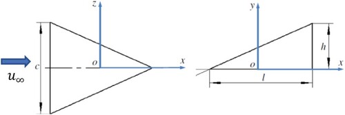
In the present numerical study, a flat plate model with a full length of $350h(700\mathrm{mm})$ and a reduced span of $40h(80\mathrm{mm})$ is used. The thickness of the flat plate model is set to zero to eliminate the effect of any leading-edge curvature discontinuity and to prevent laminar flow separation. The same micro-ramp model is placed at $145h(290\mathrm{mm})$ downstream of the leading edge. The experimental flow conditions are applied for the purpose of validation, which corresponds to unit Reynolds number $R{e}_x=2.13\times {10}^5$ and a freestream velocity $u_{\mathrm{\infty }}=10m/s$. The micro-ramp height $(h=2\mathrm{mm})$ is taken as the characteristic length of the roughness element.

2.2. Governing equations

In the numerical simulation, three-dimensional unsteady Navier-Stokes (N-S) equations for the incompressible flow are solved. To implement the embedded large-eddy simulation, RANS and LES sub-zones are pre-defined by the user and different turbulence techniques are applied in the RANS and the LES sub-zones accordingly. In the RANS sub-zone, undisturbed laminar flow is expected in front of the micro-ramp element. The intermittency transition model is therefore used for the viscous modeling, in which the Shear-Stress Transport (SST) $k-\omega$ transport equations coupled with an additional transport equation for the turbulence intermittency $\gamma$ are solved together: (1) $\begin{array}{rl}& \frac{\mathrm{\partial }(\mathrm{\rho k})}{\mathrm{\partial }t}+\frac{\mathrm{\partial }(\mathrm{\rho k}{u}_i)}{\mathrm{\partial }{x}_i}\\ & =\frac{\mathrm{\partial }}{\mathrm{\partial }{x}_j}\left({\mathrm{\Gamma }}_k\frac{\mathrm{\partial }k}{\mathrm{\partial }{x}_j}\right)+G_k-Y_k+S_k+G_b\end{array}$(1) (2) $\begin{array}{rl}& \frac{\mathrm{\partial }(\mathrm{\rho \omega })}{\mathrm{\partial }t}+\frac{\mathrm{\partial }(\mathrm{\rho \omega }{u}_i)}{\mathrm{\partial }{x}_i}\\ & =\frac{\mathrm{\partial }}{\mathrm{\partial }{x}_j}\left({\mathrm{\Gamma }}_{\omega }\frac{\mathrm{\partial }\omega }{\mathrm{\partial }{x}_j}\right)+G_{\omega }-Y_{\omega }+D_{\omega }+S_{\omega }+G_{\mathrm{\omega b}}\end{array}$(2) (3) $\begin{array}{rl}& \frac{\mathrm{\partial }(\mathrm{\rho \gamma })}{\mathrm{\partial }t}+\frac{\mathrm{\partial }(\rho u_j\gamma )}{\mathrm{\partial }{x}_j}=P_{\gamma }-E_{\gamma }+\frac{\mathrm{\partial }}{\mathrm{\partial }{x}_j}\left[\left(\mu +\frac{{\mu }_t}{{\sigma }_{\gamma }}\right)\frac{\mathrm{\partial }\gamma }{\mathrm{\partial }{x}_j}\right]\end{array}$(3)

Where, $k$ and $\omega$ are the turbulence kinetic energy and the specific dissipation rate, and $\mu$ and ${\mu }_t$ are the molecular and eddy viscosity, respectively. The terms $G_k$ and $G_{\omega }$ are generation terms that represent the production of $k$ and $\omega$. ${\mathrm{\Gamma }}_k$ and ${\mathrm{\Gamma }}_{\omega }$ represent the effective diffusivity of $k$ and $\omega$. $Y_k$ and $Y_{\omega }$ represent the dissipation of $k$ and $\omega$ due to turbulence. $D_{\omega }$ represents the cross-diffusion term. $S_k$ and $S_{\omega }$ are user-defined source terms of $k$ and $\omega$. $G_b$ and $G_{\mathrm{\omega b}}$ account for buoyancy terms. The transition source term is defined as $P_{\gamma }=F_{\mathrm{length}}\mathrm{\rho S\gamma }(1-\gamma )F_{\mathrm{onset}}$, where $S$ is the strain rate magnitude, $F_{\mathrm{length}}$ is an empirical correlation/value that controls the length of the transition region. The destruction/re-laminarization source $E_{\gamma }$ is defined as $E_{\gamma }=c_{a2}\rho \mathrm{\Omega }\gamma F_{\mathrm{turb}}(c_{e2}\gamma -1)$, where $\mathrm{\Omega }$ is the magnitude of absolute vorticity, $c_{a2}$ and $c_{e2}$ are constants. The transition onset is controlled by the function $F_{\mathrm{onset}}$.

In the LES sub-zone large-eddy simulation is employed, in which large turbulence eddies (filtered) are resolved directly from the governing equations, while small eddies (residual) are modeled by using subgrid scale (SGS) models. The filtered incompressible Navier-Stokes equations are: (4) $\begin{array}{rl}& \frac{\mathrm{\partial }\overline{u_i}}{\mathrm{\partial }{x}_i}=0\end{array}$(4) (5) $\begin{array}{rl}& \frac{\mathrm{\partial }\overline{u_i}}{\mathrm{\partial }t}+\frac{\mathrm{\partial }\overline{u_i}\overline{u_j}}{\mathrm{\partial }{x}_j}=-\frac{\mathrm{\partial }p}{\mathrm{\partial }{x}_i}+\frac{1}{\mathrm{Re}}\frac{{\mathrm{\partial }}^2\overline{u_i}}{\mathrm{\partial }{x}_i{x}_j}-\frac{\mathrm{\partial }{\tau }_{\mathrm{ij}}}{\mathrm{\partial }{x}_j}\end{array}$(5) where the effect of the small scale upon the resolved scales of the turbulence appears in the subgrid scale stress term ${\tau }_{\mathrm{ij}}\sim -2{\mu }_t\overline{S_{\mathrm{ij}}}$. ${\mu }_t$ is the subgrid scale turbulent viscosity. $\overline{S_{\mathrm{ij}}}$ is the rate-of-strain tensor for the resolved scale defined by $\overline{S_{\mathrm{ij}}}=\frac{1}{2}\left(\frac{\mathrm{\partial }\overline{u_i}}{\mathrm{\partial }{x}_j}+\frac{\mathrm{\partial }\overline{u_j}}{\mathrm{\partial }{x}_i}\right)$. $\overline{u_i}$ is the large-scale flow velocity vector. $p$ is he pressure. $\mathrm{Re}$ is the flow Reynolds number.

The SGS model is especially important when computing flows with a laminar to turbulent transition, in which a LES formulation that automatically provides zero eddy-viscosity for laminar shear flow is desirable. The simplest model to provide this functionality is the WALE (Wall-Adapting Local Eddy-viscosity) model, which has been used successfully in a variety of applications of classical LES (Jee et al., 2018; Kim et al., 2020; Lin et al., 2021). However, the main disadvantage of the WALE model is its excessive computing cost for wall-bounded flows, particularly for industrial flows at moderate to high Reynolds numbers. Wall-modeled large eddy simulation is an alternative to the classical LES+WALE model, which reduces the stringent and $\mathrm{Re}$ number-dependent grid resolution requirements of the classical LES (Bose & Park, 2018; De Vanna et al., 2022; Larsson et al., 2016). However, the WMLES method does not provide zero eddy-viscosity for flows with constant shear. To overcome this deficiency, an algebraic WMLES model with enhanced formulation (referred to as the WMLES $S-\mathrm{\Omega }$ model) is used here. It enables the computation of transitional effects in the boundary layer and avoids the overly large eddy-viscosity production in separating shear layers. In the WMLES $S-\mathrm{\Omega }$ model, the eddy viscosity ${\mu }_t$ is calculated with the use of a hybrid length scale $\mathrm{\Delta }$: (6) $\begin{array}{rl}{\mu }_t& =\rho \cdot \text{min}[{(\kappa d_w)}^2,{(C_{\mathrm{Smag}}\mathrm{\Delta })}^2]\\ & \cdot (S-\mathrm{\Omega })\cdot \{1-\text{exp}[-{(y^{+}/25)}^3]\}\end{array}$(6) where, $d_w$ is the wall distance, $y^{+}$ is the wall normal spacing, $S$ is the strain rate, $\mathrm{\Omega }$ is the vorticity magnitude, and $\mathrm{\kappa and}{C}_{\mathrm{Smag}}$ are constants. The WMLES $S-\mathrm{\Omega }$ model is based on a modified grid scale $\mathrm{\Delta }$ to account for the grid anisotropies in wall-modeled flows: (7) $\begin{array}{r}\mathrm{\Delta }=\min (\max (C_w\cdot d_w;C_w\cdot h_{\max };h_{\mathrm{wn}});h_{\max })\end{array}$(7) where $h_{\max }$ is the maximum edge length for a rectilinear hexahedral cell, $h_{\mathrm{wn}}$ is the wall-normal grid spacing, and $C_w$ is a constant.

More details on above numerical models can be found in the Theory Guide of Commercial CFD solver ANSYS Fluent.

One best practice in implementing the ELES method in roughness-induced transition simulation is that the use of the WMLES $S-\mathrm{\Omega }$ model in the LES sub-zone is found to perform considerably better than the WALE model. The former results in close agreement with the experimental data, while the latter separates immediately after the RANS-LES interface and overpredicts the separation length, thus fails to capture the vortices evolution and turbulent wedge development correctly further downstream. The same error of the WALE model in a NASA hump flow simulation was reported by Menter et al. (Menter et al., 2011) and was deemed to be attributed to the lack of mesh resolution. Therefore, the ELES with the WMLES $S-\mathrm{\Omega }$ model in the LES sub-zone is determined to be the most suitable approach for this type of roughness-induced transition simulation. The unsteady flow details behind the roughness element are captured properly and the overall computing cost is reduced substantially compared to the DNS method (as described in next Section). It could be used as an alternative numerical tool for wall-bounded industrial flows with medium to high Reynolds numbers, allowing an effective compromise between the cost and the accuracy.

2.3. Computational setup

To setup the computational domain for the model, a Cartesian coordinate system is established with its origin at the center of the roughness element, $x,y,z$ representing the streamwise (length), normal (height) and spanwise (width) directions respectively as shown in Figure 1, and $u,v,w$ representing the three corresponding velocity components. The flat plate model is placed on the bottom of the domain and extends across the entire span of the domain. The domain inlet is located at $50h$ upstream of the plate's leading edge, and the outlet is at the trailing edge of the plate. The overall computational domain extent is defined as $-195h\le x\le 200h$, $0h\le y\le 50h$, and $-20h\le z\le 20h$. The pre-defined LES sub-zone is created to capture the complex flow phenomena and the transition process around the micro-ramp element. It has an extent of $-10h\le x\le 80h$, $0h\le y\le 5h$, and $-8h\le z\le 8h$ and aligns with the measurement domain in the wind tunnel tests (Ye et al., 2016a). In the experimental study, flow in the measurement domain exhibits a strong unstable vortical structure and a clear visualization of the induced laminar to turbulent transition. The rest of the computational domain has been divided into three RANS sub-zones - RANS-Front, RANS-Middle and RANS-Back - based on their physical positions relative to the micro-ramp. A structured hexahedral mesh is generated in each sub-zone with a non-conformal mesh resolution across the interfaces between the sub-zones. The grid parameters in each zone are listed in Table 2.

Table 2. Grid parameters for sub-zones.

Sub-zone	$\mathrm{\Delta }{\mathit{y}}_{\mathit{wall}}^{+}$	$\mathrm{\Delta }{\mathit{x}}^{+},\mathrm{\Delta }{\mathit{z}}^{+}$
LES	0.7	0.06-35
RANS-Front	0.7	7-124
RANS-Middle	0.7	1-51
RANS-Back	0.7	11-99

Here, non-dimensional cell spacings are defined as: (8) $\begin{array}{r}\mathrm{\Delta }{x}^{+}=\frac{u_{\tau }\mathrm{\Delta }x}{\nu },\mathrm{\Delta }{y}^{+}=\frac{u_{\tau }\mathrm{\Delta }y}{\nu },\mathrm{\Delta }{z}^{+}=\frac{u_{\tau }\mathrm{\Delta }z}{\nu }\end{array}$(8) where $u_{\tau }=\sqrt{\frac{{\tau }_w}{\rho }}$ is the friction velocity, ${\tau }_w$ is the wall shear stress, $\rho$ is the air density, and $\nu$ is the kinematic viscosity. $\mathrm{\Delta }{x}^{+}$ and $\mathrm{\Delta }{z}^{+}$ are evaluated as: (9) $\begin{array}{r}\mathrm{\Delta }{x}^{+}=\mathrm{\Delta }{z}^{+}=\frac{\mathrm{\Delta }{y}^{+}\mathrm{\Delta }\sqrt{A_{\mathrm{cell}}}}{\mathrm{\Delta }y}\end{array}$(9) $A_{\mathrm{cell}}$ is the magnitude of the local cell face area. The cell spacings of $\mathrm{\Delta }{x}^{+},\mathrm{\Delta }{y}^{+},\mathrm{\Delta }{z}^{+}$ are satisfied sufficiently with the specific mesh resolution requirements in the RANS and the LES formulations, which is $\mathrm{\Delta }x=\frac{{\delta }_{99}}{10}$, $\mathrm{\Delta }z=\frac{{\delta }_{99}}{20}$ and $\mathrm{\Delta }{y}^{+}\le 1$ for the WMLES method. In addition, a refined mesh in LES sub-zone has been tested to verify the mesh independence in the present study.

The total mesh size is approximately eight million cells, which shows significant reduction compared to the DNS for the incompressible flow around roughness elements (as shown in Table 1). The near-field grid around the micro-ramp roughness element and the refined mesh in the LES sub-zone are displayed in Figure 2, including the close-up views of the non-conformal mesh cross the front and back RANS-LES interfaces. The physical positions of the RANS sub-zones are also displayed in Figure 2.

Figure 2. Mesh around the micro-ramp (a) and in the LES/RANS sub-zones (b).

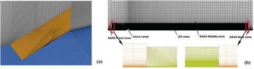
In the RANS sub-zones, velocity inlet and pressure outlet boundary conditions are set accordingly. Two spanwise boundaries are set as symmetry corresponding to the reduced spanwise extent. A non-slip condition is set on the flat plate and the micro-ramp. In the embedded LES sub-zone, the top, side, and downstream interfaces between the RANS and the LES zones are treated as common interior interfaces. The upstream interface where the flow leaves the RANS sub-zone and enters the LES sub-zone is critical due to the necessity of converting the modeled turbulence kinetic energy in the RANS zone into resolved energy in the LES zone. Different techniques of generating turbulent content at the RANS-LES interface have been proposed in open literatures (Shur et al., 2014). In the present numerical simulation, a vortex generation method is employed with a vortex number of 4250 based on the local vortex size and the RANS-LES interface area. More details on the vortex generation method and its application in the ELES can be found in Lin et al (Lin et al., 2021).

In the RANS sub-zones, a second order upwind scheme is applied for spatial discretization of momentum and turbulent quantities. A pressure-velocity coupling scheme is used to solve the averaged Navier–Stokes governing equations. In the embedded LES sub-zone, large turbulence scales are resolved directly, and small turbulence scales are modeled using the WMLES $S-\mathrm{\Omega }$ model. A central differencing scheme is utilized for momentum spatial discretization. A bounded second order implicit method is used for temporal discretization in both the RANS and the LES zones. The user-specified fixed time advancement method with a time step $\mathrm{\Delta }t=1\times {10}^{-6}s$ is selected to achieve a Courant number $\mathrm{CFL}<1$ in the LES part of the domain, which is defined as: (10) $\begin{array}{r}\mathrm{\Delta }t\le \mathrm{CFL}\frac{\sqrt[3]{{(\mathrm{cell}\mathrm{volume})}_{\min }}}{u_{\mathrm{\infty }}}\end{array}$(10) The ELES continues from a steady state three-dimensional RANS based on the intermittency transition modeling to reduce the time cost of the transient procedure. The transient computation lasts for $T{u}_{\mathrm{\infty }}/h=900$. Computation for the statistical quantities lasts for $T{u}_{\mathrm{\infty }}/h=2600$, which is sufficient to yield a smooth averaging of turbulent quantities. Commercial CFD package ANSYS is employed in present study with Fluent for the solving and ICEMCFD for meshing. Roughly 200 CPU hours are used based on 300 cluster codes.

2.4. Undisturbed laminar boundary layer

Before proceeding with the study of the flow behavior induced by the micro-ramp roughness element, it is necessary to determine the characteristics of the undisturbed boundary layer that is established on the flat plate. In the experimental study the boundary layer developing on a flat plate without the micro-ramp is characterized by its velocity profile obtained from an average of 200 uncorrelated tomographic PIV measurement samples (Ye et al., 2016a). In the present numerical study, a two-dimensional transitional boundary layer simulation is performed over an undisturbed smooth flat plate model. The velocity profiles at four typical streamwise locations ($x/h=-10,0,5,200$) are plotted in Figure 3 using normalized velocity ($u/u_{\mathrm{\infty }}$) and wall normal spacing unit ($\eta =u_{\mathrm{\infty }}y/\nu$). The results also compare with the theoretical solution based on Blasius’ solution for a zero-pressure-gradient boundary layer and the experimental data (Ye et al., 2016a).

Figure 3. Undisturbed boundary layer velocity profiles.

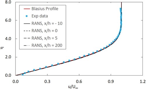
A perfect agreement of the velocity profiles between the four streamwise locations is achieved indicating that the flat plate boundary layer has reached a laminar self-similar state. The close agreement between the experimental, the numerical, and the theoretical results confirms the laminar regime of the undisturbed boundary layer over the entire test domain (up to $x/h=200$). The boundary layer integral parameters are analysed and validated successfully by the experimental data, as shown in Table 3. Here, ${\delta }^{\ast }$ and $\theta$ are the displacement and momentum thickness of the boundary layer, respectively. $H$ is the shape factor $H={\delta }^{\ast }/\theta$. $R{e}_x=u_{\mathrm{\infty }}x/\nu$, $R{e}_h=u_{h}h/\nu$ and $R{e}_{\theta }=u_{\mathrm{\infty }}\theta /\nu$ are the Reynolds numbers based on streamwise location, roughness element height, and momentum thickness, respectively, and $u_h$ is the Blasius streamwise velocity assessed at roughness height $h$.

Table 3. Laminar boundary layer integral parameters.

	u∞ (m/s)	δ99 (mm)	δ* (mm)	θ (mm)	h/δ99	H	Rex	Reh	Reθ
Exp (Ye et al., 2016a)	10	3.26	1.14	0.44	0.61	2.59	2.13E+05	1170	302
ELES	10	3.31	1.04	0.41	0.60	2.53	2.13E+05	1170	303

3. Results and discussions

In this section, time-mean flow characteristics are presented in Section 3.1 to visualize the overall flow behavior and the associated instability development and eddy topology induced by the micro-ramp roughness element. Instantaneous vortical structure and turbulent wedge development are discussed in Section 3.2 to provide details of the evolution of vortices and transition mechanism. A statistical analysis on the flow fluctuations is performed in Section 3.3 to give further details and evidence regarding the vortex evolution and the turbulence development behind the micro-ramp. In Section 3.4, the aerodynamic performance of the flat plate model with an isolated micro-ramp roughness element is analysed and the effect of the roughness-induced transition on drag forces is evaluated.

3.1. Time-mean flow field

3.1.1. Time-averaged velocity field

The topology of the time-averaged flow field has been demonstrated by the mean velocity and mean vorticity fields in the experimental study. In the present numerical study, the contours of non-dimensional time-averaged streamwise velocity $\mathrm{AveUx}=u/u_{\mathrm{\infty }}$ in the $y-z$ planes downstream of the micro-ramp are illustrated together with the mean velocity streamlines at streamwise locations of $x/h=5,15,53$ in Figure 4. The corresponding experimental measurements (Ye et al., 2016a) are also shown for comparison.

Figure 4. Time-averaged streamwise velocity contours and streamlines in y-z planes (Left: present ELES; Right: experiment (Ye et al., 2016a)).

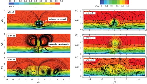
It is found that the numerical data agree well with the experimental measurement. In the near-wake region ($x/h=5$), a pair of primary streamwise vortices with counter-rotating motion is formed, producing an upwash motion in the central symmetry plane ($z/h=0$) and a lateral downwash at $z/h\approx \pm 0.6$. This pattern has been reported in many studies conducted in subsonic/supersonic turbulent boundary layers (Babinsky et al., 2009; Klebanoff et al., 1992; Sun et al., 2012) and agrees well with the experimental observation in Figure 4 (right column). Beneath the primary vortex pair, a much weaker secondary pair of counter-rotating vortices is visualized, which has an opposite direction of rotation with respect to the primary pair and induces a downwash motion in the symmetry plane close to the wall. Secondary vortices were also observed in the hypersonic laminar micro-ramp wake (Tirtey et al., 2011). A saddle point where flow stagnates is formed between the two vortex pairs at approximately $y/h=0.4$ and $z/h=0$ (shown as a white dot in Figure 4 at $x/h=5$). A lower position of the saddle point was found in the experiment ($y/h=0.2$ and $z/h=0$). The secondary vortex pair was not visualized clearly at $x/h=5$ in the experimental study. It may be due to the limitation of the measurement technique in the very near-wake.

In the downstream location of $x/h=15$, both the primary and the secondary vortex pairs are observed clearly in the numerical simulation and the experimental measurement. The saddle point ($y/h=1.1$) and the vortex core positions ($y/h=1.8$) are lifted compared to those at the position of $x/h=5$. Below the saddle point, the secondary vortex pair induces a downwash motion in the symmetry plane resulting in high momentum fluid (with a twofold increase in velocity magnitude) directed downwards to the wall. Away from the symmetry plane, a lateral upwash motion produced by the secondary vortex pair generates low momentum fluid, which is associated with the velocity deficit at the side. The inflectional velocity profile in the near-wall region will cause flow fluctuations and instability, which may trigger vortex generation and boundary layer transition. Further downstream, the primary vortex pair is lifted further with decreased strength. The tertiary vortex pair makes its first appearance outwards next to the secondary vortex pair at $x/h=25$ (not shown here). The superimposed upwash motion caused by the secondary and the tertiary vortex pairs together generates unsteady ejection events, which is hypothesized as the precursor to the laminar-to-turbulent transition. At approximately $x/h=53$, a fourth and fifth vortex pairs appear outwards. The downwash and upwash motions of the fluid due to the generation of vortex pairs appear in turn along the span, resulting in streamwise velocity streak. The velocity streamlines for the primary vortex at $x/h=53$ have risen to the upper edge of the LES sub-zone. The core of the secondary vortex pair has moved further from the wall and outwards significantly, which widens the high-speed region close to the wall.

3.1.2. Time-averaged vorticity field

The time-averaged vorticity field in the LES sub-zone is rendered on an iso-surface of the non-dimensional time-averaged streamwise vorticity ${\omega }_x^{\ast }={\omega }_{x}h/u_{\mathrm{\infty }}=0.06$ (orange color for clockwise rotation vortices) and ${\omega }_x^{\ast }=-0.06$ (blue color for anticlockwise rotation vortices) in Figure 5. The vortical structure and the vortex pairs occurrence (left in Figure 5) present a nice agreement with the experimental observation (right in Figure 5).

Figure 5. Iso-surface contour of time-averaged streamwise vorticity (Left: present ELES; Right: experiment Ye et al., 2016a).

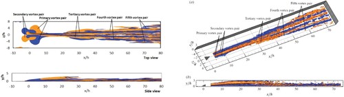
In the near wake region, two pairs of counter-rotating structures corresponding to the primary and the secondary vortex pair appear to be active from the most upstream location around the micro-ramp due to the flow separation. One pair is a closely spaced pair of vortex filaments (the primary vortex pair) and is formed in the near wake. It spirals upward at the rear of the roughness and trails downstream; the other pair wraps around the front of the roughness forming a pair of streamwise vortices (the secondary vortex pair) and extends downstream (Klebanoff et al., 1992). The tertiary vortex pair appears outwards at approximately $x=25h$. Further downstream, a fourth and a fifth vortex pair are observed further outwards, due to the mutual induction effect of the neighboring vortices. The side view of Figure 5 illustrates clearly the two vortex layers formed behind the micro-ramp: the top layer containing the primary vortices emanates from the trailing edge of the micro-ramp and eventually becomes unstable with the formation of Kelvin–Helmholtz (K–H) vortices (Acarlar & Smith, 1987); while the bottom layer is established initially by the combined action of the primary and the secondary vortex pair in the near wake region, then the primary vortices lift up and diffuse downstream, and the bottom layer sustains further downstream by the combined effect of the secondary and the tertiary vortex pair.

3.1.3. Momentum deficit and turbulence recovery

Momentum deficit and turbulence recovery have been observed and evaluated in previous studies on micro-ramp wake flow (Ghosh et al., 2010; Sun et al., 2014b; Ye et al., 2016a). In the present study, the non-dimensional time-averaged streamwise velocity profiles $u/u_{\mathrm{\infty }}$ in the symmetry plane ($z/h=0$) are plotted at four streamwise locations ($x/h=5,15,40\mathrm{and}70$). The undisturbed boundary layer profiles and the experimental data (Ye et al., 2016a) are plotted together for validation, as shown in Figure 6.

Figure 6. Time-averaged streamwise velocity profiles in the symmetry plane.

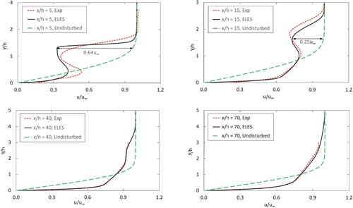
It is visualized that the micro-ramp wake exhibits an overall deficit with respect to the laminar reference. At $x/h=5$, a maximum velocity deficit of approximately $0.64U_{\mathrm{\infty }}$ is observed at the location $y/h=1.3$, which overpredicts slightly the experimental data ($0.60U_{\mathrm{\infty }}$ at $y/h=1.2$) and implies the underprediction of the shear layer mixing close to the wall in the ELES. The large discrepancy between the experimental and the numerical velocity profiles at $x/h=5$ may be attributed to the unresolved vortices in the separated near-wake flow due to the insufficient mesh resolution immediately behind the micro-ramp. The turbulence recovery process is dominated by large-scale mixing across the shear layers, as indicated by the rapid decrease of the velocity deficit at $x/h=15$, where a maximum deficit of $0.25U_{\mathrm{\infty }}$ is observed at $y/h=1.7$. The shear layer mixing is predicted quite well in the near-wall region but slightly overpredicted away from the wall at $x/h=15$, presenting a underpredicted velocity deficit with respect to the experimental data ($0.3U_{\mathrm{\infty }}$ at $y/h=1.8$). At $x/h=40\text{ and }70$, there is no minimum velocity observed in the profile due to the wake diffusion induced by the shear layer mixing. It is evident that the boundary layer has transitioned from laminar to turbulent. A typical velocity profile in the turbulent flow is visualized, and the boundary layer thickness is much larger at $x/h=40\text{ and }70$ compared to the laminar flow reference. In general, the ELES exhibits particularly good agreement of streamwise velocity profiles in the far-wake turbulent flow regime ($x/h=40,70$).

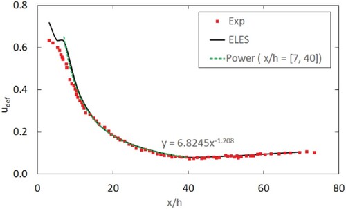
The turbulence recovery is dominated by the K–H vortex structures and can be quantified by visualizing the streamwise evolution of the maximum momentum deficit: (11) $\begin{array}{r}{u}_{\mathrm{def}}=\frac{{(u_{\mathrm{BL}}(y)-u(y))}_{\max }}{u_{\mathrm{\infty }}}\end{array}$(11) where $u_{\mathrm{BL}}$ is the velocity of the undisturbed laminar boundary layer. The calculated $u_{\mathrm{def}}$ is plotted together with the experimental data (Ye et al., 2016a) in Figure 7. The same trend of $u_{\mathrm{def}}$ evolution between the numerical and the experimental data is found: a rapid decrease of the maximum velocity deficit from $0.6U_{\mathrm{\infty }}$ to $0.1U_{\mathrm{\infty }}$ occurs within the range of $7<x/h<35$; beyond this range, the velocity deficit stays constant at approximately $0.1U_{\mathrm{\infty }}$. However, the ELES overpredicts the maximum velocity deficit in the near-wake region up to $x/h=10$, which is also observed in Figure 6 at $x/h=5$ and may be attributed to the insufficient local mesh resolution. Sun et al. (Sun et al., 2014b) observed that the streamwise evolution of the maximum velocity deficit follows a power-law type decay in a supersonic turbulent boundary layer. In the present analysis, a power-law relation is fitted to the maximum velocity deficit profile in the range of $x/h=[7,40]$: (12) $\begin{array}{r}{u}_{\mathrm{def}}=6.8245(x/h{)}^{-1.208}\end{array}$(12) The recovery rate of 1.208 is considerably larger than the value of 0.73–0.78 reported by Sun et al. (Sun et al., 2014b) and 1.06 reported by (Ye et al., 2016a), indicating an overpredicted momentum mixing and a more rapid turbulent recovery, particularly in the near-wake region.

Figure 7. Evolution of maximum velocity deficit.

3.1.4. Instability and transition

The nature of the flow around a three-dimensional roughness element with an inflectional velocity profile in the immediate downstream vicinity of the roughness has been well documented (Klebanoff et al., 1992). To validate qualitatively the flow behavior discovered by the flow-visualization studies, the spanwise distribution of the time-averaged velocity $u/u_{\mathrm{\infty }}$ (Figure 8) and the velocity fluctuation intensity $u^{\mathrm{\prime }}/u_{\mathrm{\infty }}\times 100\mathrm{\%}$ (Figure 9) at streamwise locations of $x/h=15\mathrm{and}45$ are displayed at wall-normal distances of $y/h=[0.5,2.5]$.

Figure 8. Spanwise distribution of time-averaged velocity at streamwise locations $\mathit{x}/\mathit{h}=15\mathit{and}45$.

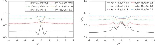
Figure 9. Spanwise distribution of velocity fluctuation at streamwise locations $\mathit{x}/\mathit{h}=15\mathit{and}45$.

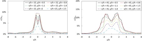
The spanwise distributions of $u/u_{\mathrm{\infty }}$ in Figure 8 clearly demonstrate the inflectional velocity profiles and the associated instability characteristic behind the roughness element. Two vortex sets are indicated: the primary trailing vortex pair in the top layer causes an upwash motion in the central symmetry plane. It transfers momentum away from the plate and results in lower velocity magnitude at $z/h=0$. The secondary vortex pair in the bottom layer transfers momentum towards the plate and results in higher velocity magnitude at the $z/h=0$ plane. Moving downstream from $x/h=15\mathrm{to}45$, the primary vortices move upwards and diffuse rapidly. The combined action of the secondary and the tertiary vortex pair presents high momentum sideward in the bottom layer.

The spanwise distribution of the velocity fluctuation intensity $u^{\mathrm{\prime }}/u_{\mathrm{\infty }}\times 100\mathrm{\%}$ in Figure 9 supports the interpretation on the evolution of vortices at a supercritical Reynolds number (Klebanoff et al., 1992): a high-level unsteadiness with double peaks is visualized and extends laterally and further away from the plate surface, which implies the presence of hairpin vortices and is consistent with the experimental observations (Klebanoff et al., 1992). It was suggested that the high intensity of $u^{\mathrm{\prime }}$ may reflect a higher concentration of the vortices as well as a stronger vortex interaction in the disturbed boundary layer at a supercritical Reynolds number (Klebanoff et al., 1992). The lateral extent of the time-averaged velocity and its fluctuation intensity moving downstream is associated with the eddy shedding and the vortex interaction. It is beyond the characteristic length of the roughness element, as shown in Figures 8 and 9. Klebanoff et al. (Klebanoff et al., 1992) also suggested that the hairpin eddies may not result from a rolling-up of the trailing vortex filaments, but rather an additional eddy system that develops nonlinearly from an unstable inflectional time-mean flow established by the pre-existing vortices. It is hypothesized that the hairpin eddies are intrinsic to the transition occurrence and the turbulence development.

According to the Law of the Wall, the turbulent boundary layer can be characterized by a logarithmic equation: $u^{\ast }=C_1\ln (y^{\ast })+C_2$, here, $y^{\ast }$ is the non-dimensional wall normal distance, $y^{\ast }=u_{\tau }y/\nu$; $u^{\ast }$ is the non-dimensional velocity, $u^{\ast }=u/u_{\tau }$; $u_{\tau }$ is the friction velocity, $\nu$ is the kinematic viscosity, $C_1$ and $C_2$ are constants. To visualize the transition onset and the development of the turbulent regime, the velocity profiles are plotted on a semi-logarithmic scale together with the experimental data in Figure 10. Six streamwise locations are chosen corresponding to the turbulence evolution process. At $x/h=5,15\mathrm{and}25$, the velocity profiles feature a large momentum deficit region due to the wake, while at $x/h=40,53\mathrm{and}70$, a power-law fitted line for the upper part of the profile indicates the presence of a fully turbulent layer complying with the log law. In general, at all inspected streamwise locations but at $x/h=5$, the ELES results present close agreement with the experimental data at the wall unit $y^{\ast }>30$. The discrepancy in the near-wall region $y^{\ast }<30$ implies the inherent feature of RANS modeling in the WMLES. At $x/h=5$, the velocity profile exhibits large discrepancy from the experimental measurement at $y^{\ast }<100$, which is deemed to be attributed to the unsolved vortices in the near-wake separated flow. Spanwise mesh refinement may ease the discrepancy but at the cost of significantly increased computing cost. It is found that the local discrepancy in the very near-wake does not affect the downstream transitional and turbulent flow development, as described in following sections. From $x/h=40$, the boundary layer flow exhibits a consistent turbulent regime in both the numerical and the experimental observations.

Figure 10. Streamwise velocity semi-log profile in symmetry plane $\mathit{z}/\mathit{h}=0$.

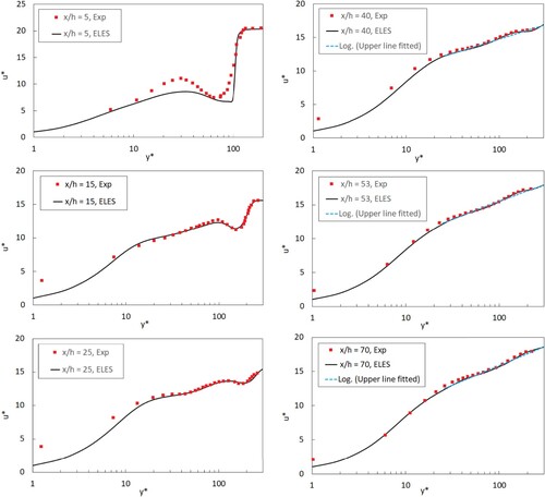
One best practice of implementing the ELES method in present case is to apply the most suitable mesh resolution to enable the effective compromise between the computing cost and the accuracy. The mesh resolution used in the present study is validated to be most suitable for this type of roughness-induced transition simulation due to its significant reduction in the computing cost and the overall good validation of the results. Through the review of existing DNS for different types of roughness elements as shown in Table 1, it is found that the ELES presents a similar level of accuracy to that in DNS, though the presence of local discrepancy in the near-wake.

3.2. Instantaneous flow field and vortex structure

3.2.1. Vortex evolution and transition mechanism

The formation and growth of vortices induced by roughness elements was deemed to be associated with the triggering mechanism of boundary layer transition (Citro et al., 2015; Ergin & White, 2006; Sun et al., 2012; Ye et al., 2016a). Extensive discussion in literatures had focused on shear layer instability beyond the roughness elements of a range of geometries, such as a micro-ramp in a supersonic turbulent boundary layer (Li & Liu, 2011; Zhou et al., 2016), circular cylinders (Ergin & White, 2006), and hemispherical caps (Acarlar & Smith, 1987; Citro et al., 2015). To visualize the vortical structure development behind a micro-ramp in a laminar incompressible flow, a three-dimensional contour of a vortex detection criterion (${\lambda }_2$ criterion) (Acarlar & Smith, 1987; Citro et al., 2015) within the LES zone is presented in Figure 11. The pattern of K–H vortices and its evolution in the wake is clearly visualized on an iso-surface of ${\lambda }_2=-5\times {10}^5$ colored by the non-dimensional time-averaged streamwise velocity $u/u_{\mathrm{\infty }}$. The ELES reproduces the experimental measurement (Ye et al., 2016a) and provides more clearer details on the vortex evolution.

Figure 11. Instantaneous vortex structure detected by the iso-surface of ${\mathit{\lambda }}_2$ criterion (Left: present ELES; Right: experiment (Ye et al., 2016a)).

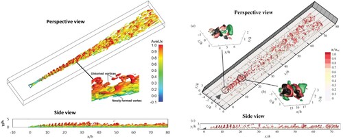
In the very near-wake $(x/h<5)$, the shear layer flow is dominated by the primary streamwise vortex pair and exhibits a quasi-steady behavior with no evidence of shear layer fluctuations. Arc-shaped vortices can be clearly observed in the shear layer, which emanate from the micro-ramp trailing edge due to K–H instability. Moving downstream, the vortices stretch under the shearing motion and lift due to the upwash motion, forming a train of large-scale lift-up hairpin-like vortices in the top layer, as shown in the side view in Figure 11. At $x=15h$, the full ring vortices is formed, as observed in experimental visualization studies (Sun et al., 2014a; Ye et al., 2016a). Downstream of the pairing region, up to approximately $x/h=30$, the vortices rapidly break down. As a result, the ring-shaped hairpin vortices are distorted and split into irregular fragments, as shown in the zoomed view in Figure 11. Starting from $x/h=25$, in the bottom layer new hairpin-like vortices are formed and shift away from the symmetry plane (zoomed view in Figure 11). They spread out along spanwise moving downstream and eventually occupy the fully developed turbulent boundary layer. The position of the occurrence of these vortex structures coincides with the range of the tertiary vortex pair detection. The newly formed vortices are observed to stay at a relatively constant wall-normal position and show no clear periodicity from their pattern (Figure 11, side view), which agrees well with the experimental observation. The global vortical structure behind the micro-ramp roughness element resembles a wedge shape.

From both the experimental visualization and the present numerical simulation, the process of vortex evolution and the turbulent wedge formation behind the micro-ramp roughness element show similar behavior to the development of turbulent spots where the perturbations trigger shear layer instability and eventually lead to transition (Durbin & Wu, 2007; Singer, 1996). Therefore, the present numerical study validates the hypothesis that the newly developed hairpin vortex system causes the occurrence of boundary layer transition and the turbulence development. The good agreement between the numerical and the experimental data also validates the capability of the ELES method in capturing the details of the vortical structure development behind the roughness element.

3.2.2. Flow separation

Any roughness element in the boundary layer will generate an adverse pressure gradient, which may cause flow to separate and a system of vortices to create. For the isolated micro-ramp element in an incompressible laminar flow, a cap-like upstream separation bubble and a shuttle-like downstream separation bubble are observed by using the iso-surface of a small negative streamwise velocity ($u=-1\times {10}^{-4}{u}_{\mathrm{\infty }}$) and colored by the non-dimensional streamwise Reynolds stress $\frac{u{}^{\mathrm{\prime }}u{}^{\mathrm{\prime }}}{u_{\mathrm{\infty }}^2}$, as shown in Figure 12.

Figure 12. Mean separation bubble around the micro-ramp.

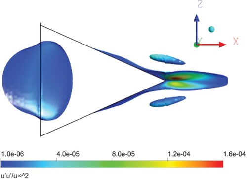
The small value of $u{}^{\mathrm{\prime }}u{}^{\mathrm{\prime }}$ in the separated flow indicates that the separation is quite steady and mild. A quasi-steady primary streamwise vortex pair is generated in the near wake, corresponding to the separation region immediately behind the micro-ramp. It spirals upward at the rear of the roughness, trails, and breaks up downstream. The secondary vortex pair is formed wrapping around the front of the roughness, corresponding to the separation region therein. It will then evolve downstream and interact with new-formed tertiary vortices, and eventually cause the boundary layer transition and the turbulence development. The vortical structure formation downstream is sourced from the flow separation and the resultant flow fluctuations around the micro-ramp.

3.3. Statistical analysis of flow fluctuations

3.3.1. Velocity fluctuation

The laminar to turbulent transition process can be characterized by analysing statistically the flow fluctuations, such as the root mean square (rms) of streamwise velocity fluctuations ($u{}^{\mathrm{\prime }}$) and wall-normal velocity fluctuations ($v{}^{\mathrm{\prime }}$). Contours of non-dimensional velocity fluctuations $\mathrm{RMSUx}=u{}^{\mathrm{\prime }}/u_{\mathrm{\infty }}\times {10}^2$ and $\mathrm{RMSUy}=v{}^{\mathrm{\prime }}/u_{\mathrm{\infty }}\times {10}^2$ are demonstrated at various $y-z$ planes in Figures 13 and 14, respectively. Six streamwise locations of $x/h=5,15,25,40,53\mathrm{and}70$ are chosen to compare with the experimental measurement (Ye et al., 2016a). Contour lines of the time-averaged streamwise velocity are superimposed with the cross-sectional contours. The ELES results are exhibiting good agreement with the experimental measurements at all locations except at $x/h=5$.

Figure 13. Contours of rms streamwise velocity fluctuations in y-z planes (Left: present ELES, Right: experiment (Ye et al., 2016a)).

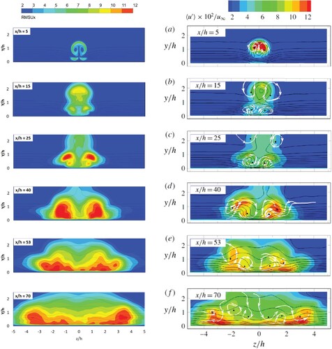
Figure 14. Contours of rms wall-normal velocity fluctuations in y-z planes (Left: present ELES, Right: experiment (Ye et al., 2016a)).

At $x/h=15$, the upwash (in the symmetry plane) and downwash (in the side plane) motions induced by the primary vortex pair contribute to the strong streamwise and wall-normal velocity fluctuations along the wake centerline and the interface between the wake and the freestream. However, at $x/h=5$ only the contribution from the downwash motions in the side plane is captured in the numerical result. It may be attributed to the unresolved vortices in the separated near-wake flow due to the insufficient mesh resolution immediately behind the micro-ramp, as observed in Figures 6, 7 and 10. Traveling downstream, the maximum of the velocity fluctuations due to the primary vortices are lifted progressively, accompanied with a significant decay and a rapid wake recovery in the vortex breakdown region ($x/h\approx [25,35]$). From $x/h=40$ onwards, the velocity fluctuations in this region become negligible ($u{}^{\mathrm{\prime }},v{}^{\mathrm{\prime }}<5\text{\% }{u}_{\mathrm{\infty }}$).

In the bottom layer (beneath the wake), downwash motion produced by the secondary vortex pair transports high momentum fluid towards the wall in the central plane and the mean velocity contour lines was demonstrated downward bending near the wall in the symmetry plane at $x/h=15$ in Figure 13. The downwash motion produces a higher wall shear resulting in an increased level of streamwise velocity fluctuations. Away from the symmetry plane, low-speed regions with an upward bending of the mean velocity contour lines are observed from $x/h=15$ onwards, which is caused by the ejection events induced by the secondary vortex pairs. Further downstream, a tertiary vortex pair is formed and produces an inflectional velocity profile jointly with the secondary pair, as visualized in the velocity contours lines at $x/h=25$. Unlike the decay process of the Kelvin–Helmholtz (K-H) instability in the wake (top layer), the velocity fluctuations in the bottom layer persist until the farthermost downstream location in the LES sub-zone ($x/h=80$). It is deemed that the velocity fluctuations generated in the near-wall region is the physical condition that sustains the turbulence cascade leading to transition. As a result, the onset of a turbulent wedge is observed in this range ($x/h=[25,80]$).

A pair of symmetrical peaks of streamwise and wall-normal velocity fluctuations can be observed at approximately $y/h=1$ at locations of $x/h=25,40\mathrm{and}53$ in Figures 13 and 14. They are resulted from turbulent momentum mixing at the turbulent/non-turbulent interface due to the formation of large-scale hairpin vortex structures. The magnitudes of the wall-normal velocity fluctuations are approximately half of the streamwise velocity fluctuations. The cross-sectional area occupied by the turbulent fluctuations increases linearly in the spanwise direction due to the lateral evolution of the newly formed hairpin vortices and causes the formation of the turbulent wedge. Near the downstream edge of the LES sub-zone ($x/h=70$), the flow exhibits a more homogeneous contour of the streamwise and the wall-normal velocity fluctuations. However, two symmetrical peaks of velocity fluctuations at the bottom of the turbulent wedge ($y/h\approx 1,z/h\approx \pm 3.5$) are still noticeable, indicating the sustained propagation of the hairpin vortices towards the undisturbed laminar boundary layer. Brinkerhoff and Yaras (Brinkerhoff & Yaras, 2014) observed that the regeneration of wavepackets of hairpin vortices at the edge of the turbulent spot dominates its lateral spreading. The present ELES validates the hypothesis that the spanwise propagation of the turbulent/non-turbulent interface is induced by the formation of large coherent hairpin structures rather than small-scale isotropic turbulent fluctuations.

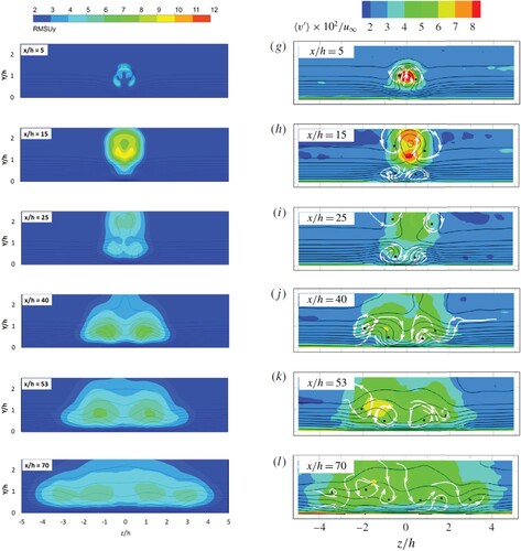
The evolutionary pattern of the velocity fluctuations can also be visualized in its contour view in the symmetry plane $z/h=0$ as shown in Figure 15. In the near wake region $x/h=[3,20]$, the streamwise velocity fluctuation is dominated by the shear layer instability, while beyond $x/h=25$, the streamwise velocity fluctuation becomes dominant in the near-wall region due to the formation of large-scale hairpin vortices and sustains until the edge of the LES zone. At the farthermost downstream location ($x/h=80$), the distribution of the streamwise velocity fluctuation tends to become more homogeneous and the maximum in the symmetry plane approaches the value of approximately $0.11u_0$, consistent with the values reported in the turbulent boundary layer (Klebanoff et al., 1955; Spalart, 1988).

Figure 15. Contour of streamwise velocity fluctuations in the x-y plane at $\mathit{z}/\mathit{h}=0$ (Top: present ELES, Bottom: experiment (Ye et al., 2016a)).

3.3.2. Turbulence production

The source of velocity fluctuations can be characterized with the production of turbulence kinetic energy $P$, which is expressed by the shear production term in the turbulence kinetic energy ($\mathrm{TKE}$) budget, defined as $P=-\overline{{u^{\mathrm{\prime }}}_i{u^{\mathrm{\prime }}}_j}\frac{d\overline{u_j}}{d\overline{x_i}}$. The spatial distribution of the non-dimensional turbulence production $P^{\ast }=\frac{P}{u_{\mathrm{\infty }}^3/h}\times {10}^4$ in the $y\text{--}z$ plane is shown at six streamwise locations of $x/h=5,15,25,40,53\mathrm{and}70$ in Figure 16, together with the contour lines of rms streamwise velocity fluctuations and the corresponding experimental measurements for comparison.

Figure 16. Contours of the turbulence production in y-z planes (Left; present ELES; Right: experiment (Ye et al., 2016a)).

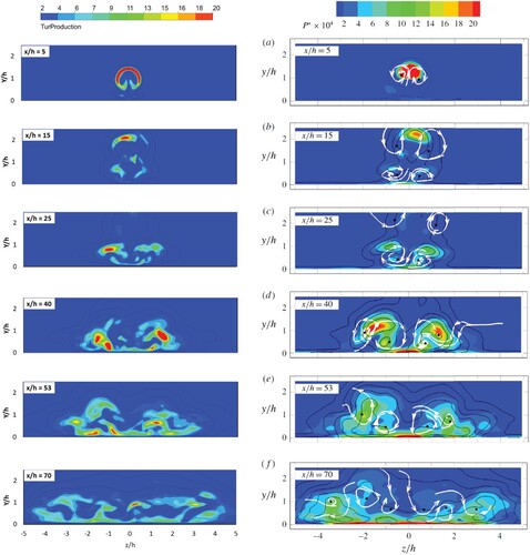
The ELES shows good agreement with the experimental measurements. Within the shear layer dominated by the arc/ring-shaped primary vortices (K-H vortices), a maximum of $P^{\ast }$ is attained in the top layer (Figure 16, $x/h=5\mathrm{and}15$). Moving downstream, with the primary vortex breakdown and turbulence recovery, the strength of turbulence production in the top shear layer decreases rapidly and becomes negligible from $x/h=25$. At $x/h=25$, a peak of production near the symmetry plane is identified in the bottom layer due to the excess wall shear caused by the secondary vortex pair. Two side peaks are also observed outwards and upwards, which is caused by the sidewise ejections induced by the combined effect of the secondary and the tertiary vortex pair. The side peaks in turn maintains the sidewise shear layer. The lateral shear layer attributes to the onset of velocity fluctuations, transferring mean flow energy into turbulence kinetic energy and strengthening the turbulence production in the bottom shear layer. Further downstream ($x/h>25$), the overall pattern of the turbulence production $P^{\ast }$ becomes more complex: the strength of the turbulence production intensifies and concentrates along the turbulent wedge border. Multi-peaks are observed either in the near-wall region towards the symmetry plane (clearly resolved from $x/h=25$ onwards) or displaying sidewards. From $x/h=40$ onwards, lateral movement of the turbulence production peaks follows the spanwise propagation of the turbulent wedge, indicating a self-similar behavior for the turbulent wedge front. At $x/h=70$, the turbulence production becomes relatively homogeneous, and the peaks are observed in the near-wall region due to the excess wall shear and the inflectional instability produced.

From both the numerical and the experimental studies, it is concluded that the turbulence production is established in the near-wake region due to the combined effect of flow ejections and the excess wall shear and then the pattern sustains independently. Moving downstream, large-scale hairpin vortex structures are generated within the turbulence wedge, which actively transfers mean flow kinetic energy into turbulence and contributes to the propagation of turbulent fluctuations into the laminar region.

3.3.3. Turbulent wedge

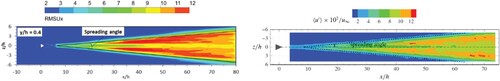
Schubauer and Klebanoff (Schubauer & Klebanoff, 1956) performed an experimental investigation on the transition process behind three-dimensional roughness elements and found that the transition starts from perturbations in the laminar flow as spots which then grow and move downstream. The transition region is developed containing turbulent patches and finally merges to form a wedge-shaped completely turbulent region consisting of a fully turbulent core bounded by an intermittent region. In the present numerical study, the contour of rms streamwise velocity fluctuation ($u{}^{\mathrm{\prime }}/u_{\mathrm{\infty }}\times {10}^2$) at a chosen $x-z$ plane ($y/h=0.4$) demonstrates the formation of the turbulent wedge behind the micro-ramp, as shown in Figure 17. The predicted turbulent wedge (left in Figure 17) shows good agreement with the experimental measurements (right in Figure 17). The fully turbulent core and the intermittent region in the turbulent wedge is clearly visible and an averaged border line between the laminar and the turbulent flow is recognized. The turbulent wedge presents a significant increase of streamwise velocity fluctuation level compared to the undisturbed laminar region. A dramatic decrease of velocity fluctuation level is found when moving from the turbulent core towards the border of the turbulent wedge. A half spreading angle of the turbulent wedge is found to be approximately $5^{\circ }$ in Figure 17, which agrees well with the value of ${4.6}^{\circ }$ found in the experimental data (Ye et al., 2016a) and ${5.2}^{\circ }$ reported in the numerical simulation by Brinkerhoff and Yaras (Brinkerhoff & Yaras, 2014).

Figure 17. Turbulent wedge formation (Left: present ELES; Right: experiment (Ye et al., 2016a).

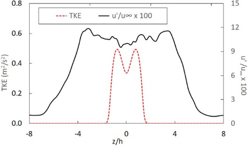
The spanwise distribution of the rms streamwise velocity fluctuation ($u{}^{\mathrm{\prime }}/u_{\mathrm{\infty }}\times {10}^2$) and the Turbulence kinetic energy ($\mathrm{TKE}$) at a far downstream position of $x/h=70$ and $y/h=0.4$ are plotted in Figure 18. $\mathrm{TKE}$ exhibits the highest level within the symmetrical turbulent core and then decreases sharply in the intermittent and laminar region. The rms streamwise velocity fluctuation, however, sustains a higher level across the turbulent core and the intermittent region in the turbulent wedge and then drops abruptly in the laminar region. The present ELES results agree well with the observation in the DNS study (De Tullio, 2013) and the experimental study (Ye et al., 2016a).

Figure 18. Profiles of velocity fluctuation and TKE in the turbulent wedge.

3.4. Effects on aerodynamic performance

The micro-ramp trips the laminar to turbulent transition in the boundary layer and inevitably causes viscous drag increase. In our numerical simulation, the drag coefficient of the flat plate model with and without the micro-ramp is calculated in all flow sub-zones, as listed in Table 4. Here, $C_{d\mathrm{\_t}}$ is the total drag coefficient. The reference area for the drag coefficient is the total area of the flat plate model.

Table 4. Effect of micro-ramp roughness element on drag coefficient ${\mathit{C}}_{\mathit{d}\mathrm{\_}\mathit{t}}$.

Sub-zone	${\mathit{C}}_{\mathit{d}\mathrm{\_}\mathit{t}}$ with ramp	${\mathit{C}}_{\mathit{d}\mathrm{\_}\mathit{t}}$ without ramp	Drag increment
RANS-Front	$1.20\times {10}^{-3}$	$1.20\times {10}^{-3}$	0%
RANS-Middle	$2.14\times {10}^{-4}$	$2.14\times {10}^{-4}$	0%
RANS-Back	$5.40\times {10}^{-4}$	$3.82\times {10}^{-4}$	41%
LES	$2.58\times {10}^{-4}$	$1.43\times {10}^{-4}$	81%

In the RANS-Front and the RANS-Middle zones, a laminar boundary layer is sustained with or without the micro-ramp roughness element resulting in zero increment in the drag coefficient. In the LES zone, laminar to turbulent transition occurs behind the micro-ramp and a turbulent wedge is developed downstream. A significant drag increase is therefore observed in the LES zone (81%) and the subsequent RANS-Back zone (41%). The large drag increment in the LES zone is attributed to the excess wall shear produced by the interaction of the secondary and the tertiary vortices. The total drag force $(C_{d\mathrm{\_t}})$ in the LES sub-zone consists of the drag caused by the micro-ramp element itself $(C_{d\mathrm{\_r}})$, and the drag on the flat plate only $(C_{d\mathrm{\_f}})$. Further analysis finds that the drag force caused by the micro-ramp element itself is quite small ($C_{d\mathrm{\_r}}=1.17\times {10}^{-5}$), approximately $4.5\mathrm{\%}$ of the total drag in the LES zone. Most drag in the LES zone is generated on the flat plate ($C_{d\mathrm{\_f}}=2.47\times {10}^{-4}$), which is attributed to the transitional/turbulent boundary layer flow. The same conclusion was found in the study of a hypersonic transition induced by isolated roughness elements (Duan & Xiao, 2017).

4. Conclusions

A numerical investigation on the incompressible transitional boundary-layer flow behind an isolated three-dimensional micro-ramp roughness element mounted on a flat plate is performed. The embedded LES combining the intermittency transition model in the RANS sub-zone and the WMLES $S-\mathrm{\Omega }$ model in the LES sub-zone is employed for the first time. Numerical results on the time-averaged flow field, the instantaneous flow field and the statistical flow fluctuations are analysed and validated thoroughly by the existing experimental measurements.

In summary, at the supercritical Reynolds number, the disturbed boundary layer behind the micro-ramp consisted of two vortex regions that interact with each other - an inner region dominated by two sets of vortices and an outer region dominated by the eddy shedding. The two sets of vortices in the inner region originate from the flow separation around the roughness element: one set is a closely spaced primary streamwise vortex pair forming in the near wake and spiraling upward at the rear of the roughness; the other set consists of horseshoe-shaped vortices close to the surface, wrapping around the front of the roughness and forming a pair of secondary streamwise vortices in the bottom shear layer. The primary vortex pair dominates in the range of $x/h=[2,30]$ and forms a train of hairpin-like vortices in the top shear layer moving downstream, and then rapidly distorts and splits into irregular fragments at around $x/h=30$. The secondary vortex pair sustains in the bottom layer and induces a central downwash motion and lateral upwash motion causing a velocity streak. Starting from $x/h=25$, hairpin-like tertiary vortices are formed and develops downstream with spanwise spreading. The newly formed hairpin vortices in the near-wall region occupy the fully-developed turbulent wedge. The present numerical simulation validates the hypothesis that the combined action of the secondary and the tertiary streamwise vortices in the bottom shear layer causes an inflectional velocity profile with excess wall shear and strong velocity fluctuations in the near-wall region, and the resultant hairpin eddies trigger the transition and the turbulence development.

In general, the computational results show good agreement with the experimental data for nearly all the measured flow characteristics and quantities, which indicates the capability of the ELES method of capturing the boundary layer transition process and the turbulence vortex development induced by three-dimensional roughness elements. Compared to the most commonly used DNS method and the classical LES method, the present zonal hybrid RANS/LES method combined with the WMLES $S-\mathrm{\Omega }$ model shows a significant reduction of the computing cost while maintaining great overall accuracy. The main limitation of the present methodology is the flow discrepancy in the near-wake $(x/h<10)$ due to the insufficient local mesh resolution. However, this discrepancy is within the local area and will not affect the downstream transitional and turbulent flow development. Therefore, it is concluded that the ELES combining an intermittency transition model in the RANS sub-zone and a WMLES $S-\mathrm{\Omega }$ model in the LES sub-zone is an efficient simulation tool for the wall-bounded industrial flows at moderate to high Reynolds number that allows effective compromise between flexibility, cost, and accuracy. The best practice of implementing the present ELES methodology can be used in other types of roughness-induced transitional and turbulent flow simulation, such as the compressible subsonic and supersonic flow applications.

Data availability statement

The data that support the findings of this study are available from the corresponding author Y. Lin [[email protected]] upon reasonable request.

Disclosure statement

No potential conflict of interest was reported by the author(s).

Additional information

Funding

This research did not receive any specific grant from funding agencies in the public, commercial, or not-for-profit sectors.

References

- Acarlar, M. S., & Smith, C. R. (1987). A study of hairpin vortices in a laminar boundary layer. Part 1. Hairpin vortices generated by a hemispherical protuberance. Journal of Fluid Mechanics, 175(-1), 1–41. https://doi.org/10.1017/S0022112087000272
- Babinsky, H., Li, Y., & Pittford, C. W. (2009). Micro ramp control of supersonic oblique shockwave/boundary-layer interactions. AIAA Journal, 47(3), 668–675. https://doi.org/10.2514/1.38022
- Belkhou, H., Russeil, S., Dbouk, T., Mobtil, M., Bougeard, D., & Francois, N.-Y. (2019). Large Eddy Simulation of boundary layer transition over an isolated ramp-type micro roughness element. International Journal of Heat and Fluid Flow, 80, 108492. https://doi.org/10.1016/j.ijheatfluidflow.2019.108492
- Bernardini, M., Pirozzoli, S., & Orlandi, P. (2012). Compressibility effects on roughness-induced boundary layer transition. International Journal of Heat and Fluid Flow, 35, 45–51. https://doi.org/10.1016/j.ijheatfluidflow.2012.02.007
- Berry, S. A., Auslender, A. H., Dilley, A. D., & Calleja, J. F. (2001). Hypersonic boundary-layer trip development for Hyper-X. Journal of Spacecraft and Rockets, 38(6), 853–864. https://doi.org/10.2514/2.3775
- Blinde, P. L., Humble, R. A., Van Oudheusden, B. W., & Scarano, F. (2009). Effects of micro-ramps on a shock wave/turbulent boundary layer interaction. Shock Waves, 19(6), 507–520. https://doi.org/10.1007/s00193-009-0231-9
- Bose, S. T., & Park, G. I. (2018). Wall-modelled large-eddy simulation for complex turbulent flows. Annu. Rev. Fluid Mech, 50(1), 535–561. https://doi.org/10.1146/annurev-fluid-122316-045241
- Brinkerhoff, J. R., & Yaras, M. I. (2014). Numerical investigation of the generation and growth of coherent flow structures in a triggered turbulent spot. Journal of Fluid Mechanics, 759, 257–294. https://doi.org/10.1017/jfm.2014.538
- Choudhari, M., Li, F., & Edwards, J. (2009). Stability analysis of roughness array wake in a high-speed boundary layer. 47th AIAA Aerospace Science Meeting, Orlabndo, Jan, 2009, AIAA Paper, 2009–0170. https://doi.org/10.2514/6.2009-170.
- Choudhari, M., Li, F., Wu, M., Chang, C. L., Edwards, J., Kegerise, M., & King, R. (2010). Laminar-turbulent transition behind discrete roughness elements in a high-speed boundary layer. AIAA Paper, 2010–1575. https://doi.org/10.2514/6.2010-1575
- Citro, V., Luchinia, P., Giannettia, F., & Auterib, F. (2015). Boundary-layer flows past a hemispherical roughness element: DNS, global stability and sensitivity analysis. IUTAM ABCM Symposium on Laminar Turbulent Transition. Procedia IUTAM, 14, 173–181. https://doi.org/10.1016/j.piutam.2015.03.038
- De Tullio, N. (2013). Receptivity and transition to turbulence of supersonic boundary layers with surface roughness [PhD thesis]. University of Southampton.
- De Vanna, F., Bernardini, M., Picano, F., & Benini, E. (2022). Wall-modelled LES of shock-wave/boundary layer interaction. International Journal of Heat and Fluid Flow, 98), https://doi.org/10.1016/j.ijheatfluidflow.2022.109071
- Dong, H., Liu, S., Geng, X., Liu, S., Yang, L., & Cheng, K. (2019). Numerical and experimental investigation into hypersonic boundary layer transition induced by roughness elements. Chinese Journal of Aeronautics, 32(3), 559–567. https://doi.org/10.1016/j.cja.2018.12.004
- Duan, Z., & Xiao, Z. (2017). Hypersonic transition induced by three isolated roughness elements on a flat plate. Computers & Fluids, 157, 1–13. https://doi.org/10.1016/j.compfluid.2017.08.006
- Duan, Z. W., Xiao, Z. X., & Fu, S. (2014). Direct numerical simulation of hypersonic transition induced by an isolated cylindrical roughness element. Science China Physics, Mechanics & Astronomy, 57(12), 2330–2345. https://doi.org/10.1007/s11433-014-5556-4
- Durbin, P., & Wu, X. (2007). Transition beneath vortical disturbances. Annual Review of Fluid Mechanics, 39(1), 107–128. https://doi.org/10.1146/annurev.fluid.39.050905.110135
- Elsinga, G. E., & Westerweel, J. (2012). Tomographic-PIV measurement of the flow around a zigzag boundary layer trip. Experiments in Fluids, 52(4), 865–876. https://doi.org/10.1007/s00348-011-1153-8
- Ergin, F. G., & White, E. B. (2006). Unsteady and transitional flows behind roughness elements. AIAA Journal, 44(11), 2504–2514. https://doi.org/10.2514/1.17459
- Ghosh, S., Choi, J. I., & Edwards, J. R. (2010). Numerical simulations of effects of micro vortex generators using immersed-boundary methods. AIAA Journal, 48(1), 92–103. https://doi.org/10.2514/1.40049
- Jee, S., Joo, J., & Lin, R. S. (2018). Toward cost-effective boundary layer transition computations with large-eddy simulation. Journal of Fluids Engineering, 140(11).
- Kegerise, M., King, R., Owens, L., Choudhari, M., Norris, A., Li, F., & Chang, C. L. (2012). An experimental and numerical study of roughness-induced instabilities in a Mach 3.5 boundary layer. Tech. Rep. NATO RTO AVT.
- Kim, M., Lim, J., Kim, S., Jee, S., & Park, D. (2020). Assessment of the wall-adapting local eddy-viscosity model in transitional boundary layer. Computer Methods in Applied Mechanics and Engineering, 371, 113287. https://doi.org/10.1016/j.cma.2020.113287
- Klebanoff, P. S., Cleveland, W. G., & Tidstrom, K. D. (1992). On the evolution of a turbulent boundary layer induced by a three-dimensional roughness element. Journal of Fluid Mechanics, 237, 101–187. https://doi.org/10.1017/S0022112092003379
- Klebanoff, P. S., Schubauer, G., & Tidstrom, K. D. (1955). Measurements of the effect of two dimensional and three-dimensional roughness elements on boundary-layer transition. J. Aerospace Sci, 22, 803–804.
- Klebanoff, P. S., & Tidstrom, K. D. (1972). Mechanism by which a two-dimensional roughness element induces boundary-layer transition. The Physics of Fluids, 15(7), 1173–1188. https://doi.org/10.1063/1.1694065
- Larsson, J., Kawai, S., Bodart, J., & Bermejo-Moreno, I. (2016). Large eddy simulation with modeled wall-stress: Recent progress and future directions. Mechanical Engineering Reviews, 3(1), 15-00418–15-00418. https://doi.org/10.1299/mer.15-00418
- Li, Q., & Liu, C. (2011). Implicit LES for supersonic micro-ramp vortex generator: New discoveries and new mechanisms. Modelling and Simulation in Engineering, 2011, 1–15. https://doi.org/10.1155/2011/934982
- Lin, Y., Wang, J., & Savill, M. (2021). Embedded large eddy simulation of transitional flow over NACA0012 aerofoil. Proceedings of the Institution of Mechanical Engineers, Part G: Journal of Aerospace Engineering, 235(2), 189–204. https://doi.org/10.1177/0954410020939797
- Mary, I., & Sagaut, P. (2002). Large Eddy Simulation of Flow Around an Airfoil Near Stall. AIAA Journal, 40(6), https://doi.org/10.2514/2.1763
- Mathey, F. (2008). Aerodynamic noise simulation of the flow past an airfoil trailing-edge using a hybrid zonal RANS-LES. Computers & Fluids, 37(7), 836–843. https://doi.org/10.1016/j.compfluid.2007.04.008
- Menter, F. R., Schütze, J., & Kurbatskii, K. A. (2011). Scale-Resolving Simulation Techniques in Industrial CFD. 6th AIAA Theoretical Fluid Mechanics Conference, 27 - 30 June 2011, Honolulu, Hawaii. AIAA 2011-3474.
- Quemere, P., & Sagaut, P. (2002). Zonal multi-domain RANS/LES simulations of turbulent flows. International Journal for Numerical Methods in Fluids, 40(7), 903–925. https://doi.org/10.1002/fld.381
- Redford, J. A., Sandham, N. D., & Roberts, G. T. (2010). Compressibility effects on boundary layer transition induced by an isolated roughness element. AIAA Journal, 48(12), 2818–2830. https://doi.org/10.2514/1.J050186
- Richez, F., Mary, I., Gleize, V., & Basdevant, C. (2008). Zonal RANS/LES coupling simulation of a transitional and separated flow around an airfoil near stall. Theoretical and Computational Fluid Dynamics, 22(3-4), 305–315. https://doi.org/10.1007/s00162-007-0068-8
- Rizzetta, D., & Visbal, M. (2006). Direct numerical simulations of flow past an array of distributed roughness elements. 36th AIAA Fluid Dynamics Conference and Exhibit, 5 - 8 June 2006, San Francisco, California. AIAA 2006-3527.
- Schubauer, G. B., & Klebanoff, P. S. (1956). Contributions on the mechanics of boundary-layer transition. NACA Tech. Rep, 1289.
- Shur, M. L., Spalart, P. R., & Strelets, M. K. (2014). Synthetic turbulence generators for RANS-LES interfaces in zonal simulations of aerodynamic and aeroacoustic problems. Flow, Turbulence and Combustion, 93(1), 63–92. https://doi.org/10.1007/s10494-014-9534-8
- Singer, B. A. (1996). Characteristics of a young turbulent spot. Physics of Fluids, 8(2), 509–521. https://doi.org/10.1063/1.868804
- Spalart, P. R. (1988). Direct simulation of a turbulent boundary layer up to Reθ = 1410. Journal of Fluid Mechanics, 187, 61–98. https://doi.org/10.1017/S0022112088000345
- Sun, Z., Scarano, F., Van oudheusden, B. W., Schrijer, F. F. J., Yan, Y., & Liu, C. (2014a). Numerical and experimental investigations of the supersonic micro ramp wake. AIAA Journal, 52(7), 1518–1527. https://doi.org/10.2514/1.J052649
- Sun, Z., Schrijer, F. F. J., Scarano, F., & Van oudheusden, B. W. (2012). The three-dimensional flow organization past a micro-ramp in a supersonic boundary layer. Physics of Fluids, 24, 1–22.
- Sun, Z., Schrijer, F. F. J., Scarano, F., & Van oudheusden, B. W. (2014b). Decay of the supersonic turbulent wakes from micro-ramps. Physics of Fluids, 26, 1–21.
- Tani, I. (1969). Boundary-layer transition. Annual Review of Fluid Mechanics, 1(1), 169–196. https://doi.org/10.1146/annurev.fl.01.010169.001125
- Tirtey, S. C. (2008). Characterization of a transitional hypersonic boundary layer in wind tunnel and flight conditions [PhD thesis]. Von Karman Institute for Fluid Dynamics.
- Tirtey, S. C., Chazot, O., & Walpot, L. (2011). Characterization of hypersonic roughness-induced boundary-layer transition. Experiments in Fluids, 50(2), 407–418. https://doi.org/10.1007/s00348-010-0939-4
- Whitehead, A. H. Jr (1969). Flowfield and drag characteristics of several boundary-layer tripping elements in hypersonic flow. NASA, TND-5454.
- Ye, Q., Schrijer, F., & Scarano, F. (2016a). Boundary layer transition mechanisms behind a micro-ramp. J. Fluid Mech, 793, 132–161. https://doi.org/10.1017/jfm.2016.120
- Ye, Q., Schrijer, F., & Scarano, F. (2016b). Geometry effect of isolated roughness on boundary layer transition investigated by tomographic PIV. International Journal of Heat and Fluid Flow, 61, 31–44. https://doi.org/10.1016/j.ijheatfluidflow.2016.05.016
- Zhou, Y., Zhao, Y., Xu, D., Chai, Z., & Liu, W. (2016). Numerical investigation of hypersonic flat-plate boundary layer transition mechanism induced by different roughness shapes. Acta Astronautica, 127, 209–218. https://doi.org/10.1016/j.actaastro.2016.05.027
- Zhou, Z., Wang, Z., & Fan, J. (2010). Direct numerical simulation of the transitional boundary-layer flow induced by an isolated hemispherical roughness element. Computer Methods in Applied Mechanics and Engineering, 199(23-24), 1573–1582. https://doi.org/10.1016/j.cma.2010.01.004