Near surface assessment of New capital city using geophysical techniques

ABSTRACT

The Egyptian government announced the creation of a brand new capital city to address Cairo’s rapid population expansion and improve the quality of life for citizens, which is thought to have a strong demand for housing. In this study, we focused on the application of geophysical techniques, specifically Electrical Resistivity Tomography (ERT) and Very Low Frequency Electromagnetic Method (VLF-EM), to investigate the shallow subsurface in the New Capital city in Egypt. The study area is located in the eastern part of Cairo and is characterised by Oligocene and Miocene rocks. The ERT profiles reveal four geoelectrical layers based on resistivity values, with the first layer (Resistivity >300 Ω.m) interpreted as sand and conglomerate on the surface or basalt below. The second layer (100–300 Ω.m) is identified as sandstone, while the third layer (15–100 Ω.m) is interpreted as humid sandstone. The fourth layer (1–15 Ω.m) is characterised as shale. The abrupt changes in resistivity values horizontally indicate the probability of subsurface structures, including faults. The VLF-EM method is used to identify faults and cracks in the earth’s crust. The results provide information on the size, shape, and depth of both shallow and deep subterranean conductors. Anomalies of high conductivity suggest fault or fracture zones influencing underlying strata.

KEYWORDS:

• The New capital city
• ERT method
• VLF method
• faults

1. Introduction

Capital cities are national symbols of their countries. They control the political authority of the nation and its seat of government, and they typically serve as its primary social and economic hub as well. The nation’s capital rises to importance as the nation’s most prosperous city, while other cities’ growth is in some way constrained. Cairo has long served as Egypt’s capital for nearly to a century. The Greater Cairo major city, on the other hand, now has a population of close to 20 million and is projected to reach 40 million by 2050. This information might serve as a key impetus for the Egyptian government to consider building a new capital. The goal of the new capital city is to create a sense of national identity and a worldwide, smart city for the future.

The present-day geomorphological structure and spatial distribution of the several lithologic units are the results of the complicated tectonic setting of the Cairo-Suez District, which is a region of northeastern Egypt (Moustafa et al. 1985). Dawod et al. (2018), describes and analyzes the overall spatial location of such a massive development activity from geodetic and environmental points of view. Six main geological structures exist. The main geological feature is the Hagul formation that occupies more than half of the study area. The Hagul formation consists mainly from fluviatile sand and gravel, and is locally underline by white limestone with marl. The second main geological structure, Gabel el-Ahmar formation, consists of continental vividly coloured sands, quartzite and gravel. Wadi deposits constitutes about 15% of the study area. Several folds that soft link the overlapping ends of typical faults are outcropped as soft linkage transfer zones (Henasih 2018).

The study area is located in the eastern part of Cairo. Previous, excavations and engineering works in different locations of this plateau reveal the presence of shale and marl intercalation, faults, fracture zones and frequent karstic features such as cavities, voids and sinkholes. The geology of the study area in general was discussed by Said (1962) and the observation field of the authors represent the bases of the discussion around the study area; that touches the geology, the geomorphology, stratigraphy and the structure. According to Said (1962), there are three faults sets have the same age in the Cairo-Suez district (east-west, northwest and northeast). In the new city of El Alamein, where the ERT technology added two levels, the emergence of seawater intrusion starts in the second layer as shown (Basheer and Nouran 2022). In the new administrative capital, nine Electrical Resistivity Tomography (ERT) profiles and 24 Ground Penetrating Radar (GPR) profiles were employed to identify near-surface structures at the selected building site shown in (Kotb et al. 2021). Alhussein A. Basheer et al. (2023) use electrical resistivity tomography (ERT) and shallow seismic refraction (SSR) data analysis to describe the underground geological conditions and interpret the geotechnical properties of foundation rock components in the combined services area of Madinaty, New Cairo. As Jessica Bellanova et al. (2020) demonstrate, the historical areas of Matera make an excellent outdoor laboratory for testing the ability of GPR and ERT methods to illuminate and reconstruct the geometry of buried structures. In order to estimate groundwater potential in Ilara-Mokin, Akure, Falade et al. (2019) plan to combine the very low frequency electromagnetic method (VLF-EM) and vertical electrical sounding (VES) electrical resistivity approaches.

The objectives of our study are to determine the stiffness properties of the ground and to locate cavities and dissolution features in carbonate rocks using the appropriate surface geophysical techniques (VLF and resistivity) in the New Capital city.

2. Study area and geological setting

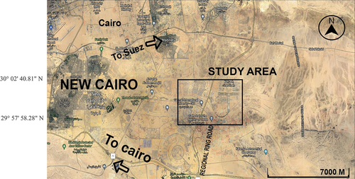
The study area is located at the heart of the New Capital in the eastern part of Cairo; it is about 60 km northeast Cairo on the Cairo-Sukhna Highway (Figure 1). Previously, karstic features like cavities, voids and sinkholes as well as faults, fracture zones and shale and marl intercalation have been discovered during excavations and engineering work in various regions of this plateau.

Figure 1. Location map of the study area.

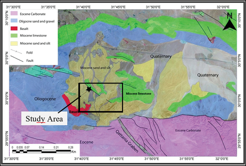
Oligocene and Miocene rocks represent the sedimentary sequence of the study area. The sedimentary sequences of the area are the products of characteristic geomorphic processes developed in response to equilibrated constructive and destructive mechanisms. The bedrock of the study area is cut through with numerous NW faults; however, the majority are geologically old and represent low risk of seismic activity. Meanwhile, most of WNW and ENE faults have not been active in the last 100 or 1000 years. In general, the most notable stratigraphic units revealed in the area east of New Cairo City between the Suez-Cairo district and the Ain Sukhna-Qattamayia district are the Miocene rocks (Figure 2). Essentially, the succession has matured into two shapes: Hommath Formation (marine carbonate and alluvial siliciclastic facies) and Hagul Formation (fluviatile sand and gravel) Said (1962), Moustafa and Abd‐Allah (1991).

Figure 2. Simplified regional geological map of the New capital city and its neighbouring.

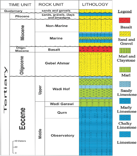
The Miocene succession is underlain by Late Oligocene-Early Miocene basaltic flow. Oligocene basalt rests above the Early Oligocene red sandstone of Al Gabal Ahmer Formation. The exposed Cretaceous rocks at the centre of Gebel Shabrawet are reflected in the stratigraphic sequence and geologic setting of the research region. There are two main rock units: (1) 250 m thick base unit composed of marl and shale and (2) an upper unit composed of Turonian to Cenomanian limestone (140 m thick). The Cairo-Suez district is largely composed of middle Eocene rocks. Sand-covered, brownish limestone with strata of sandstone are composed of the Upper Eocene rocks as described by Shukri and Akmal (1953) for 70 m thick. Uncomfortably, the Oligocene sands and gravels overlie the upper Eocene sediments, which in turn are overlain by the Miocene basal stages. The East-West faults, which formed the majority of the structural and topographic highs in the region, are the most obvious faults. They might have been created during the Pre-Cambrian Period by tangential compressive stress. Said (1962) claimed that tensional pressures were primarily responsible for the formation of the local structures. The Upper Eocene is the surface formation in the study region. Figure 3 show the generalised stratigraphic column of the study area (modified after Moustafa and Abd‐Allah 1991).

Figure 3. Generalized stratigraphic column of the study area (modified after Moustafa and Abd‐Allah 1991).

3. Methodology

In New Capital city, two geophysical techniques are used including: (1) induction technique because of the expectation of the high resistance of the medium such as earth resistivity (ERT) method and (2) non-intrusive technique used for subsurface geologic and engineering investigations based on magnetic field of radio waves such as very low frequency (VLF) method.

3.1. Electrical resistivity tomography (ERT)

The ERT is the technique of measuring certain properties of electrical fields and utilising such data in predicting the subsurface deposits or structures.

Wenner-Schlumberger array is used for conducting the ERT measurements due to its advantage of reaching profound depths with reasonable resolution for the upper parts of the profiles.

3.1.1. Data acquisition and processing

The resistivity measurements have been carried out using the SYSCAL R2 from IRIS Company. This device is designed to acquire the VES and the electrical resistivity tomography measurements. For the majority of popular electrode arrays, including Schlumberger and Wenner soundings and profiles, it computes and displays the apparent resistivity. The measurement procedure has been improved to offer the highest level of precision in actual field circumstances.

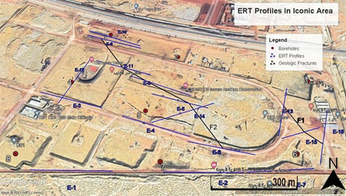
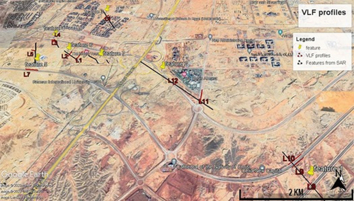
Sixteen electrical resistivity tomography profiles have been conducted at the study area (Figure 4), applying three multi-nodes boxes with 16 electrodes to measure an ERT profile with 48 electrodes, 235 metres’ length, 5 metres between each two successive electrodes to give a penetrating depth reaches to 45 metres beneath the ground surface. The ERT profiles have conducted along the free accessible roads.

Figure 4. Location map showing the conducted 16 ERT profiles at the study area.

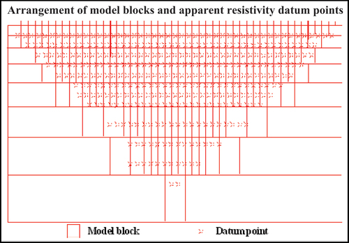
The advancement of electronic parts and PC handling have allowed to foster field resistivity gear, which incorporates countless terminals situated along a line simultaneously and which does a programmed exchanging of these cathodes for getting profiling information. This method, called resistivity imaging or ERT, tracks down applications in the ecological geography, groundwater, structural designing and antiquarianism fields. The electrical resistivity imaging yields a deciphered resistivity and profundity values got from reverse displaying programming. The multi-terminal resistivity method takes advantage of a multi-centre link with numerous cathodes (24, 48, 72, 96, …), which are connected to the ground at preset separating. The different blends of communicating (A, B) and getting (M, N) sets of terminals develop the blended sounding/profiling segment, with a greatest explored profundity, which fundamentally relies upon the complete length of the link. Different kinds of cathode setup are normal. Wenner exhibit is utilised in this work as per its high goal and enormous entered acquired profundity. The reversal program’s 2-D resistivity model is comprised of various rectangular blocks (Figure 5). The dissemination of the data of interest in the pseudo-areas is simply extraneously connected with the association of these blocks. The programme creates the dispersion and size of the blocks consequently so the quantity of model blocks does not surpass the quantity of data of interest. The profundity of the block’s base column is chosen to generally coordinate the profundity of assessment of the datum focuses with the amplest terminal separating. Ordinarily, the study is directed involving a framework in which the terminals are coordinated in a line with a proper distance between adjoining cathodes.

Figure 5. Subdivision of the subsurface into rectangular blocks to interpret the data from 2-D imaging survey using different algorithms.

3.1.2. Data interpretation

ERT is an ideal technique in geological, geotechnical engineering and environmental investigation where a comprehensive depiction of the subsurface is given in both directions vertical and horizontal.

Using advanced processing software (RES2DINV), the collected data have been visualised and modified to produce the optimum images that provide significant and accurate information about the subsurface settings. Figures from 7 to 14 show the presence of two faults in samples of the resultant 2-D imaging profiles that have been measured in the study area.

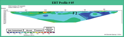
Figure 6 is show the interpreted electrical resistivity tomography of profile No. 5; it exemplifies three geoelectrical layers based on the resistivity values and the location of the layer itself as shown below. First, geoelectric layer, it is not detected due to the weathering processes. Second, geoelectric layer, small detecting of this layer due to the weathering processes. Third, geoelectric layer, this layer is characterised by moderate resistivity value (15–100 Ω.m) and will be interpreted as sandstone layer. Fourth, geoelectric layer, this layer is characterised by very low resistivity value (1–15 Ω.m). If this is at the surface, it could be interpreted as shale. If it is down the surface, it will be interpreted as fractured basalt. The abrupt changes in resistivity values horizontally in the ERT profile no. 5 reflects the probability of presence of subsurface structures (faults). Hence, inferred fault F2 could be interpreted.

Figure 6. Electrical resistivity tomography of profile no. 5.

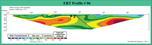
Figure 7 is show the interpreted electrical resistivity tomography of profile No. 6; it exemplifies four geoelectrical layers based on the resistivity values and the location of the layer itself as shown below. First, geoelectric layer, it is characterised by very high resistivity value reaching to more than 300 Ω.m. It is interpreted as basalt because it is below the surface. Second, geoelectric layer, this layer is characterised by moderate to high resistivity value (100–300 Ω.m) and could be interpreted as sandstone layer. Third, geoelectric layer, this layer is characterised by moderate resistivity value (15–100 Ω.m), and will be interpreted as sandstone layer. Fourth, geoelectric layer, small detecting of this layer, it is characterised by very low resistivity value (1–15 Ω.m). It will be interpreted as shale because it is at the surface. The abrupt changes in resistivity values horizontally in the ERT profile no. 6 reflects the probability of presence of subsurface structures (faults). Hence, inferred fault F2 could be interpreted.

Figure 7. Electrical resistivity tomography of profile no. 6.

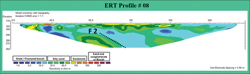
Figure 8 is show the interpreted electrical resistivity tomography of profile No. 8; it exemplifies four geoelectrical layers based on the resistivity values and the location of the layer itself as shown below. First, geoelectric layer, small detecting of this layer due to the weathering processes, it is characterised by very high resistivity value reaching to more than 300 Ω.m. It is interpreted as sand and conglomerate because it is at the surface. Second, geoelectric layer, small detecting of this layer due to the weathering processes, it is characterised by moderate to high resistivity value (100–300 Ω.m) and could be interpreted as sandstone layer. Third, geoelectric layer, this layer is characterised by moderate resistivity value (15–100 Ω.m) and will be interpreted as sandstone layer. Fourth, geoelectric layer, small detecting of this layer, it is characterised by very low resistivity value (1–15 Ω.m). If this is at the surface, it could be interpreted as shale. If it is down the surface, it will be interpreted as fractured basalt. The abrupt changes in resistivity values horizontally in the ERT profile no. 8 reflects the probability of presence of subsurface structures (faults). Hence, inferred fault F2 could be interpreted.

Figure 8. Electrical resistivity tomography of profile no. 8.

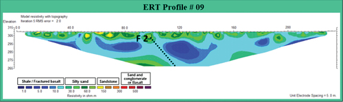
Figure 9 is show the interpreted electrical resistivity tomography of profile No. 9; it exemplifies three geoelectrical layers based on the resistivity values and the location of the layer itself as shown below. First, geoelectric layer, not detecting of this layer due to the weathering processes. Second, geoelectric layer, small detecting of this layer due to the weathering processes, it is characterised by moderate to high resistivity value (100–300 Ω.m) and could be interpreted as sandstone layer. Third geoelectric layer, this layer is characterised by moderate resistivity value (15–100 Ω.m) and will be interpreted as sandstone layer. Fourth, geoelectric layer, it is characterised by very low resistivity value (1–15 Ω.m). If this is at the surface, it could be interpreted as shale. If it is down the surface, it will be interpreted as fractured basalt. The abrupt changes in resistivity values horizontally in the ERT profile no. 9 reflects the probability of presence of subsurface structures (faults). Hence, inferred fault F2 could be interpreted.

Figure 9. Electrical resistivity tomography of profile no. 9.

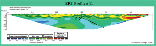
Figure 10 is show the interpreted electrical resistivity tomography of profile No. 11; it exemplifies four geoelectrical layers based on the resistivity values and the location of the layer itself as shown below. First, geoelectric layer, small detecting of this layer due to the weathering processes, it is characterised by very high resistivity value reaching to more than 300 Ω.m. It is interpreted as sand and conglomerate because it is at the surface. Second, geoelectric layer, small detecting of this layer due to the weathering processes, it is characterised by moderate to high resistivity value (100–300 Ω.m), and could be interpreted as sandstone layer. Third, geoelectric layer, this layer is characterised by moderate resistivity value (15–100 Ω.m) and will be interpreted as sandstone layer. Fourth, geoelectric layer, it is characterised by very low resistivity value (1–15 Ω.m). If this is at the surface, it could be interpreted as shale. If it is down the surface, it will be interpreted as fractured basalt. The abrupt changes in resistivity values horizontally in the ERT profile no. 11 reflects the probability of presence of subsurface structures (faults). Hence, inferred fault F2 could be interpreted.

Figure 10. Electrical resistivity tomography of profile no. 11.

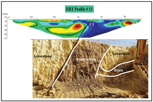
Figure 11 is show the interpreted electrical resistivity tomography of profile No. 13; it exemplifies four geoelectrical layers based on the resistivity values and the location of the layer itself as shown below. First, geoelectric layer, it is characterised by very high resistivity value reaching to more than 300 Ω.m. It is interpreted as basalt because it is below the surface. Second, geoelectric layer, it is characterised by moderate to high resistivity value (100–300 Ω.m), and could be interpreted as sandstone layer. Third, geoelectric layer, this layer is characterised by moderate resistivity value (15–100 Ω.m) and will be interpreted as sandstone layer. Fourth, geoelectric layer, it is characterised by very low resistivity value (1–15 Ω.m). If this is at the surface, it could be interpreted as shale. If it is down the surface, it will be interpreted as fractured basalt. This profile reflects severe lateral change in resistivity values that could be referred to presence of subsurface fault (F1).

Figure 11. Electrical resistivity tomography of profile no. 13 (above), geological cross section that is correlated with ERT profile (below).

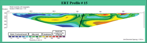
Figure 12 is show the interpreted electrical resistivity tomography of profile No. 15; it exemplifies four geoelectrical layers based on the resistivity values and the location of the layer itself as shown below. First, geoelectric layer, small detecting of this layer due to the weathering processes, it is characterised by very high resistivity value reaching to more than 300 Ω.m. It is interpreted as basalt because it is below the surface. Second, geoelectric layer, it is characterised by moderate to high resistivity value (100–300 Ω.m), and could be interpreted as sandstone layer. Third, geoelectric layer, this layer is characterised by moderate resistivity value (15–100 Ω.m) and will be interpreted as sandstone layer. Fourth, geoelectric layer, it is characterised by very low resistivity value (1–15 Ω.m). If this is at the surface, it could be interpreted as shale. If it is down the surface, it will be interpreted as fractured basalt. The abrupt changes in resistivity values horizontally in the ERT profile no. 15 reflects the probability of presence of subsurface structures (faults). Hence, inferred fault F1 could be interpreted.

Figure 12. Electrical resistivity tomography of profile no. 15.

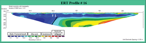
Figure 13 is show the interpreted electrical resistivity tomography of profile No. 16; it exemplifies four geoelectrical layers based on the resistivity values and the location of the layer itself as shown below. First, geoelectric layer, not detecting of this layer due to the weathering processes. Second, geoelectric layer, it is characterised by moderate to high resistivity value (100–300 Ω.m) and could be interpreted as sandstone layer. Third, geoelectric layer, this layer is characterised by moderate resistivity value (15–100 Ω.m), and will be interpreted as sandstone layer. Fourth, geoelectric layer, it is characterised by very low resistivity value (1–15 Ω.m). If this is at the surface, it could be interpreted as shale. If it is down the surface, it will be interpreted as fractured basalt. The abrupt changes in resistivity values horizontally in the ERT profile no. 16 reflects the probability of presence of subsurface structures (faults). Hence, inferred fault F1 could be interpreted.

Figure 13. Electrical resistivity tomography of profile no. 16.

3.2. Electromagnetic method VLF (very low frequency)

A geophysical method called the very low frequency electromagnetic method, or VLF-EM, makes use of electromagnetic radiation released by far-off, land-based radio transmitters. This technique has historically been used to identify faults and cracks in the earth’s crust (Eppelbaum 2021). In this work, the T-VLF (IRIS-Instrument) was used to collect data along 12 straight profiles (Figure 14). Both 23,400 and 285,000 Hz were used as our primary operational frequency. These frequencies emit radio signals that can be picked up rather easily and have a distribution that is only somewhat restricted to the azimuth. After measuring two orthogonal components of the magnetic field, one can generally deduce the tilt angle and elasticity of the vertical magnetic polarisation ellipse.

Figure 14. Location map showing the 12 VLF profiles at the study area.

3.2.1. VLF data processing and interpretation

On the VLF-EM information, the Fraser filter and the Karous-Hjelt filter (K-H filter) were utilised. To work on the flat goal of neighbourhood VLF-EM irregularities and make them all the more effectively recognisable, a discrete one-layered straight channel administrator was planned utilising the Fraser filter (Fraser 1969). This was achieved by planning a channel administrator with only one aspect. It shifts into tops as it goes along the profile because of expanding contrasts in the upsides of the in-stage part. This happens when the ongoing extremity changes. The flat inclinations are processed utilising the Fraser filter, and afterwards the information are mixed to get the most outrageous qualities over the guides. We utilised KHFFILT program in separating VLF information.

Karous and Hjelt (1983) made a sifting strategy that offers evident current densities at different profundities, delivering an attractive field like the VLF forecasts. The spatial disseminations of subsurface designs including flaws, break zones, and land guides are consequently given by the k-H filter as a pseudo segment of the bizarre current thickness. K-H esteems that are positive will show a high thickness of genuine current across the guides (high conductivity), though K-H esteems that are negative will show a lessening in current thickness (low conductivity) attributable to current get-together, which is missing in 2-D frameworks. The changed over identical current densities are addressed as scaled ued cross-segments in 2-D.

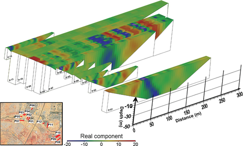
Observed data, Fraser filter results, and K-H filter outcomes along profile 1 are all shown as an example in Figure 15. The current density cross sections along profiles no. 2 to 12 are shown in Figure 16.

Figure 15. Plot showing the current density cross section along profile 1 for observed data, the Fraser filter, and the tilt angle, representing the real component of the VLF data.

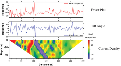
Figure 16. The current density cross sections along profile no. 2 to 12.

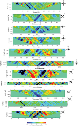
The output section is usually triangular with a maximum depth of about one-sixth of the profile’s length (Ogilvy & Lee, 1991). This is a direct outcome of the natural behaviour of the K&H filtering strategy and is not the investigation depth; nonetheless, it should be noted that this is the case owing to the dependency of examination depth on profile length in the K&H filtering method. It should be noted that this is not the depth of investigation.

Along the K-H cross sections (Figure 17), information on the size, shape and depth of both shallow and sufficiently deep subterranean conductors may be distinguished. A few subsurface anomalies of abnormally high conductivity impact horizontally both the shallow and deep cross-sections. These abnormalities may indicate fault or fracture zones that influence underlying strata.

Figure 17. The aggregation of all of the cross-sections in the research region that were produced from the K-H filter, which represents the real component of the VLF data. The cross sections are not displayed in the right locations, which are represented on the associated Google earth map.

4. Results and output

The ERT profiles exemplify four geoelectrical layers based on the resistivity values as the first geoelectric layer (Resistivity >300 Ω.m) is characterised by very high resistivity values more than 300 Ω.m. This layer when observed on the ground surface, it will be interpreted as sand with conglomerate as geological unit. If it is found below subsurface, it will be basalt as geological unit. Second geoelectric layer (100–300 Ω.m)

is characterised by moderate to high resistivity value and will be interpreted geologically as sandstone layer. Third geoelectric unit (15–100 Ω.m) is characterised by moderate resistivity value and will be interpreted as humid sandstone layer. Fourth geoelectric layer (1–15 Ω.m) is characterised by very low resistivity value, and it could be interpreted as shale.

The abrupt changes in resistivity values horizontally in the ERT profiles reflects the probability of presence of subsurface structures (faults). Furthermore, severe lateral change of resistivity values are detected on the ERT profiles (P no. 5, P no. 6, P no. 8, P no. 9 and P no. 11), (Figures 6–10). Hence, inferred fault F2 could be interpreted.

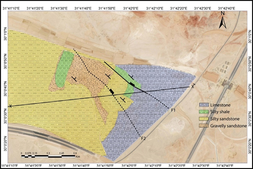
The ERT profile no. 13 reflects severe lateral change in resistivity values that could be referred to presence of subsurface fault (F1) as shown in the Figure 11 which is validated and geologically confirmed. The geophysical used techniques in this study (Resistivity, VLF) confirmed geotechnical derived results of the soil in the study area. In addition to the results proof the probability of presence of subsurface structures (two faults F1 and F2) (Figure 18). Therefore, the study area needs further engineering study and derive safe solutions for build a safe city.

Figure 18. Geological map of the study area overlies Google earth image.

5. Conclusions

In this study, we had applied ERT and VLF-EM methods to investigate the shallow subsurface at the new capital city. The ERT profiles exemplify four geoelectrical layers based on the resistivity values and the location of the layer itself. The first geoelectric layer (Resistivity >300 Ω.m), which represent the surface layer in the study area; it will be interpreted as sand and conglomerate. The second geoelectric layer has resistivity values of (100–300 Ω.m) and be interpreted as sandstone layer. While the third geoelectric layer has resistivity values of (15–100 Ω.m) and represents a humid sandstone layer. The fourth geoelectric layer has resistivity’s of (1–15 Ω.m) and could be interpreted as shale. The abrupt changes in resistivity values horizontally in the ERT profiles reflects the probability of presence of subsurface structures (faults).

The results of the VLF data method showed that, along the K-H cross-sections, information on the size, shape and depth of both shallow and sufficiently deep subterranean conductors may be distinguished. A few subsurface anomalies of abnormally high conductivity impact horizontally both the shallow and deep cross-sections. These abnormalities may indicate fault or fracture zones that influence underlying strata.

Acknowledgments

Deep acknowledgements for Geoelectric and Geothermal laboratory members, Prof. Hany Sallah and Prof. Mohamed AbdEl Zaher for helping in the measurements and assistant of geophysical scan phase.

Disclosure statement

No potential conflict of interest was reported by the author(s).

References

- Basheer AA, Abd Elhamid RM, Toni M, Ismail A. 2023. Assessment of the geo-engineering suitability of subsurface layers using ERT and SSR, a case study: combined services area of “Madinaty,” New Cairo, Egypt. J Appl Geophy. 22(1):1–16. doi: 10.21608/JAG.2023.207522.1001.
- Basheer AA, Nouran SS. 2022. Application of ERT and SSR for geotechnical site characterization: a case study for resort assessment in New El Alamein city, Egypt. NRIAG J Astron Geophys. 11(1):58–68. doi: 10.1080/20909977.2021.2023999.
- Bellanova J, Calamita G, Catapano I, Ciucci A, Cornacchia C, Gennarelli G, Giocoli A, Fisangher F, Ludeno G, Morelli G, et al. 2020. GPR and ERT investigations in Urban areas: the case-study of Matera (southern Italy). Remote Sens. 12(11):1879. doi: 10.3390/rs12111879.
- Dawod GM, Ahmed Gaber AAM, Hammed M. 2018. Geological mapping of the Central Cairo-Suez district of Egypt, using space-borne optical and radar dataset. Egypt J Remote Sens Space Sci. doi: 10.1016/j.ejrs.2018.11.004.
- Eppelbaum LV. 2021. VLF-method of geophysical prospecting a non-conventional system of processing interpretation (implementation in the Caucasian ore deposits). Earth Sci. 2:16–38. doi: 10.33677/ggianas20210200060.
- Falade AO, Amigun JO, Kafisanwo OO. 2019. Application of electrical resistivity and very low frequency electromagnetic Induction methods in groundwater investigation in Ilara-Mokin, Akure Southwestern Nigeria. Environ Earth Sci Res J. 6(3):125–135. doi: 10.18280/eesrj.060305.
- Fraser DC. 1969. Contouring of VLF-EM data. Geophysics. 34(6):958–967. Google Earth. doi: 10.1190/1.1440065.
- Henasih A. 2018. Soft-linkage transfer zones: insights from the Northern Eastern Desert, Egypt. Mar Petrol Geol. 95:265–275. doi: 10.1016/j.marpetgeo.2018.05.005.
- Karous M, Hjelt SE. 1983. Linear filtering of VLF dip-angle measurements. Geophys Prospect. 31(5):782–794. doi: 10.1111/j.1365-2478.1983.tb01085.x.
- Kotb A, Basheer AA, Nasser A, Ramah M. 2021. Utilizing ERT and GPR to distinguish structures maleficence the constructions in the New administrative capital, Egypt. Earth Sci. 10(5):234–243. doi: 10.11648/j.earth.20211005.15.
- Moustafa AR, Abd‐Allah AM. 1991. Transfer zones with an echelon faulting at the northern end of the Suez rift. Tectonics. 11(3):499–506. doi: 10.1029/91TC03184.
- Moustafa A, Yehia A, Abdel Tawab S. 1985. Structural setting of the area east of Cairo, Maadi, and Helwan. Sci Res Ser. 5:40–64.
- Said R. 1962. The geology of Egypt. Amesterdam New York: Elsevier; p. 377.