Spatiotemporal distribution of size-fractioned phytoplankton in the Yalu River Estuary, China

ABSTRACT

The grain size structure of phytoplankton has great influence on shellfish culture. The present study aimed to assess the spatial and temporal variation in the phytoplankton community structure in the Yalu River Estuary and to explore the relationship between the phytoplankton community structure and various environmental parameters in 2020. High-throughput sequencing was used in this study. The results showed that nanophytoplankton, especially Karlodinium veneficum, dominated the estuary throughout the year. The biomass ratio of picophytoplankton, nanophytoplankton, and microphytoplankton were 20:63:17 in spring, 30:44:26 in summer, 1:38:61 in autumn, and 2:45:53 in winter, respectively. Meanwhile, Dinophyta had the greatest biomass throughout the year, followed by Bacillariophyta. On the spatial dimension (Station average), COD, T, SST had a positive impact on total phytoplankton communities, and Dep had a negative impact. In the time dimension (Monthly average), the environmental factor that significantly controlled the phytoplankton community structure were NO2 and SST.

KEYWORDS:

• Eukaryotic phytoplankton
• high-throughput sequencing
• particle size and structure
• environmental factors
• Yalu River Estuary

Introduction

The Yalu River originates from the southern foot of Changbai Mountain in Jilin Province, China. It flows through Changbai, Ji’an, Kuandian, Dandong, other places and southward into the Yellow Sea. Its total length is 795 km, and it has been named for its color. It is the boundary river between China and Korea. A major hydropower resource, the Yalu River is also used for transport (especially the prolific cross-strait transport of felled forest timber), and its aquatic resources are used by riparian people. The Yalu River Estuary fishing ground is rich in such wildlife as hairtail, yellow flowers, Spanish mackerel, herring, shrimp, crab, and shellfish. In 2020, the output of shellfish aquaculture was 240,000 tons, and the shallow sea aquaculture area was 45,000 ha (Liaoning Province Fishery Statistics Annual Report 2020). However, in recent years, filter-feeding shellfish such as Ruditapes philippinarum have generally been found to grow slowly, the quality of their flesh has declined and the species is experiencing increased mortality, which limits the sustainable and healthy development of that fishery (Gu 2014; Song et al. 2017).

The phytoplankton community can be divided into several size classes with different physical properties, including three size fractions: picophytoplankton (<3 μm diameter), nanophytoplankton (3–20 μm), and microphytoplankton (20–200 μm) (Song et al. 2019a, 2020). Picophytoplankton contributes to facilitating nutrient recycling through the microbial loop in the euphotic zone (Lafond, Pinel-Alloul, and Ross 1990). Nanophytoplankton and microphytoplankton are more likely to be exported to the bottom of the estuary or are consumed by herbivores and eventually exported as fecal pellets (Legendr 1999). The size spectrum and species composition of phytoplankton are determined by many factors such as the availability of light, temperature and nutrients; competition; and parasitism (Temponeras, Kristiansen, and Moustaka-Gouni 2000; Naselli-Flores and Barone 2003). Therefore, phytoplankton structure can be considered as an integrator of environmental factors (Claustre et al. 2005).

Chlorophyll-a (Chl-a) concentration is commonly used as a test to express phytoplankton biomass because it relates directly to total production (Melack 1976). Adame reported the size-fractionated biomass (expressed as Chl-a concentration) and its implications for the dynamics of an oligotrophic tropical lake, found that it was dominated by small phytoplankton (Adame, Alcocer, and Escobar 2008). In 2012, Song et al calculated the shellfish culture capacity in the Yalu River Estuary by using the biomass of the entire phytoplankton community, which was 1480 g/m² in spring, 320 g/m² in summer, and 1100 g/m² in autumn (Song et al. 2013). In 2016, Wang used the Chl-a classification method to study size-fractionated biomass in Yalu River Estuary and found that the proportions of microphytoplankton, nanophytoplankton, and picophytoplankton were 55%, 28%, and 17%, respectively (Wang and Liu 2018). High-throughput sequencing technology can reveal highly diverse eukaryotic lineages, while significantly reducing the errors associated with species identification, particularly that of phytoplankton (Stoeck, Bass, and Nebel 2010; Faria et al. 2014). Copy number variations in rDNA are often associated with changes in body size and growth rate (Prokopowich, Gregory, and Crease 2003; Zhu et al. 2005; Godhe et al. 2008). With the change in cell size, the number of rRNA/rDNA reflects the biomass of the population (Fu and Gong 2017). Compared with the Chl-a concentration assessing method, high-throughput sequencing technology provides comprehensive and detailed information about the plankton community (Song et al. 2019a). In 2020, Song et al studied the diversity of plankton and size-fractionated biomass on Dachangshan Island in China by high-throughput sequencing technology (Song et al. 2020).

The present study aimed to assess the spatial and temporal variation in the phytoplankton community structure in the Yalu River Estuary by high-throughput sequencing technology and to explore the relationship between the phytoplankton community structure and various environmental parameters in 2020.

Materials and methods

Sample collection

16 sampling sites were set up at the Yalu River Estuary, in the northern part of the Yellow Sea (Figure 1), and samples were collected every month from March to December 2020. Since the average water depth of the surveyed sea area was about 5 m, the phytoplankton environmental DNA samples were only collected from the surface of the seawater, that was, 0.5 m water depth samples. At least 1 L of seawater was vacuum-filtered through 0.22-μm cellulose acetate membranes, which were subsequently folded and flash-frozen at −80°C until subjected to further processing in the laboratory.

Figure 1. Sampling sites in Yalu River Estuary, China.

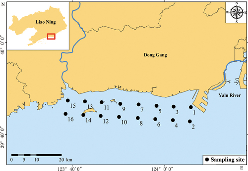
The pretreatment, preservation, detection, and quality control methods for environmental samples were implemented with reference to “Marine Survey Specifications” (GB/T12763–2007) and “Marine Monitoring Specifications” (GB17378–2007). The measured water quality parameters were: seawater depth (Dep), water temperature (T), salinity (SST), pH, and dissolved oxygen (DO). The measured water nutrient parameters were: Chl-a, chemical oxygen demand (COD), total nitrogen (TN), total phosphorus (TP), silicate (SiO₃), dissolved inorganic nutrients (nitrite [NO₂], nitrate [NO₃], ammonia nitrogen [NH₄], inorganic phosphorus [DIP], and inorganic nitrogen [DIN]), and the nitrogen to phosphorus ratio (N/P).

PCR amplification of 18S rDNA V4 variable region

The total genomic DNA from the seawater samples was extracted using the CTAB method. The primer used in this study was V4(F/R), a self-developed primer for gene amplification of the 18S rDNA V4 region of eukaryotic phytoplankton. The upstream primer was V4-F (5ʹ-GCGGTAATTCCAGCTCCAATA-3ʹ), and the downstream primer was V4-R (5ʹ-GATCCCHWACTTTCGTTCTTGA-3ʹ) (Song et al. 2016a). The primers were designed with different labels and sent to Shanghai Shenggong Biological Company for synthesis. The PCR reaction system was 50 μL, including 5 μL PCR buffer, and 8 μL dNTP mixture upstream, and 2 μL downstream primers (10 μmol/L) each, 2 μL template DNA, 2.5 U Taq DNA polymerase, and an appropriate amount of sterile water. The amplification reactions were all completed on a PE 9700 PCR instrument (PE company in the United States). The reaction conditions were 94°C pre-denaturation for 3 min; 94°C denaturation for 30 s; 58°C annealing for 45 s; 72°C extension for 45 s, 33 cycles; and 72°C extension for 5 min. PCR products were detected by 1% agarose gel electrophoresis. The sequencing libraries were generated using the NEB Next® Ultra™ DNA Library Prep Kit for Illumina (NEB, USA), according to the recommendations of the manufacturer, subsequently, index codes were added. The library quality was assessed on a Qubit@ 2.0 Fluorometer (Thermo Scientific) and an Agilent Bioanalyzer 2100 system. The library was sequenced on an Illumina HiSeq 2500 platform, and 250-bp and 300-bp paired-end reads were generated.

Data analysis

Quality control and analysis of sequencing data

The raw data obtained were spliced using FLASH software (V1.2.7, http://ccb.jhu.edu/software/FLASH/). The quality control process of the spliced sequences was carried out in Qiime software (Version 1.7.0, http://qiime.org/index.html) by intercepting and filtering to obtain valid data (Magoč and Salzberg 2011). To ensure accuracy and reliability, the high-quality data needed to account for more than 90%. Sequence analyses were performed using Uparse software (Uparse v7.0.1001, http://drive5.com/uparse/). Sequences with ≥97% similarity with a given OTU (Operational Taxonomic Units) were assigned to that OTU (Song et al. 2019b). The representative sequence for each OTU was screened for further annotation. For each, the Silva Database (http://www.arb-silva.de/) was used based on the RDP classifier algorithm (v2.2, http://sourceforge.net/projects/rdp-classifier/) to annotate taxonomic information. Protist OTUs were removed, to focus on the abundance and richness of eukaryotic phytoplankton.

Dominance index

According to related studies, the proportion of eukaryotic phytoplankton sequence numbers with different particle sizes was closer to the biomass ratio (Prokopowich, Gregory, and Crease 2003; Zhu et al. 2005; Godhe et al. 2008; Song et al. 2020), so the proportion of each eukaryotic phytoplankton sequence number is the biomass ratio. According to the relevant literature, the dominant species screened out were screened and graded according to the equivalent spherical diameter (Prokopowich, Gregory, and Crease 2003; Zhu et al. 2005; Godhe et al. 2008; Liu 2008; Xu et al. 2017; Yu 2014; Jiang 2009), and the species with phytoplankton dominance over 0.1% in each sample were taken as the overall dominant species to participate in the particle size structure statistics, that is, the sum of the eukaryotic phytoplankton sequences with an equivalent spherical diameter greater than 20 μm was used as the microphytoplankton centralized statistic; the sum of the eukaryotic phytoplankton sequences with an equivalent spherical diameter of 3–20 μm was used as the nanophytoplankton centralized statistics; the sum of the eukaryotic phytoplankton sequence with an equivalent spherical diameter of less than 3 μm was used as a centralized statistic for picophytoplankton. The proportions of different size-fractionated phytoplankton were counted according to the sequence numbers.

Dominance index Y represents the distribution of biological individuals within a community, and is also used as a parameter to determine biodiversity (Eqn 1):

(1) $Yi=\frac{ni}{N}fi,$(1)

where $n_i$ is the sum of the sequences of i algae in all samples; N is the sum of all algae sequences; and $f_i$ is the occurrence frequency of i algae in all samples. The species with dominance over 0.1% obtained at each station are taken as the overall dominant species in the cell-size biomass ratio.

Statistical analyses

The biomass proportion of each phytoplankton species (the proportion of each phytoplankton sequence number in this sample) was used to represent the proportion of phytoplankton in different particle size communities, and redundancy analysis (RAD) and principal component analysis (PCA) were performed using Canoco 5 to analyze its correlation with various environmental factors.

Results

Phytoplankton species composition

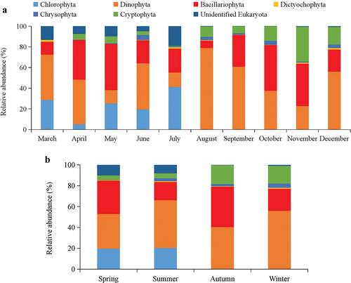
The relative abundance of Dictyochophyta, Chrysophyta, Cryptophyta, and unknown algae was low, and their biomass was smaller. The dominant nanophytoplankton species in the Bacillariophyta was Thalassiosira nordenskioeldii, and its highest dominance appeared in May. Karlodinium veneficum was the dominant nanophytoplankton species in Dinophyta, and numbers were at their greatest in September. The dominant picophytoplankton species of Chlorophyta was Ostreococcus tauri, and its dominance was greatest in July. Cryptomonadales sp. was the dominant nanophytoplankton species of Cryptophyta, and its dominance was greatest in November. The dominant nanophytoplankton species of Chrysophyta was Heterosigma akashiwo, and its dominance was greatest in June (Figure 2a). Dinophyta was the dominant group throughout the year, followed by Bacillariophyta. The species richness of the dinoflagellates was higher than that of the Bacillariophyta in all four seasons (Since the sea area freezes from January to February in winter, the on-site investigation cannot be carried out. Therefore, only the data of December can be used to represent the winter). Chlorophyta had higher relative abundance in spring and summer (Figure 2b).

Figure 2. (a) Relative abundance of phytoplankton composition (Phylum) from March to December; (b) Relative abundance of phytoplankton composition (Phylum) in all four seasons in Yalu River Estuary, China.

Dominant species in Yalu River Estuary

The monthly dominant phytoplankton species (Y > 0.02) in Yalu River Estuary were shown in Table 1. In spring, K. veneficum, Brockmanniella brockmannii, and Thalassiosira nordenskioeldii comprised the dominant biomass in phytoplankton communities. In summer, K. veneficum, O. tauri, and Gyrodinium dominans comprised the dominant biomass in phytoplankton communities. In autumn, the biomass of K. veneficum, Cryptomonadales sp., and T. curviseriata dominated. In winter, Alexandrium affine was the most dominant species. Comprehensive consideration, K. veneficum dominated the Yalu River Estuary, no matter in the frequency or dominance of the dominant species all year.

Table 1. Dominant species of phytoplankton in Yalu River Estuary, China, from March to December 2020.

Time	Species name	Y	Time	Species name	Y
March	ukaryote marine clone ME1-22*	0.14	September	Karlodinium veneficum**	0.51
	Prasinophyte sp.**	0.12		Spiniferites belerius***	0.09
	Gymnodinium aureolum***	0.10		Thalassiosira curviseriata***	0.05
	Karlodinium veneficum**	0.08		Polykrikos kofoidii***	0.04
	Thalassiosira nordenskioeldii**	0.08		Cerataulina pelagica***	0.04
	Chlorella sorokiniana**	0.06		Cryptomonadales sp.**	0.03
	Heterocapsa triquetra**	0.05		Teleaulax amphioxeia**	0.02
	Eukaryote marine clone ME1-24*	0.03		Tripos tenuis***	0.02
	Azadinium polongum**	0.03		Akashiwo sanguinea***	0.02
April	Karlodinium veneficum**	0.42	October	Thalassiosira curviseriata***	0.22
	Brockmanniella brockmannii**	0.21		Spiniferites belerius***	0.20
	Thalassiosira nordenskioeldii**	0.08		Cryptomonadales sp.**	0.12
	Eukaryote marine clone ME1-24*	0.07		Karlodinium veneficum**	0.05
	Hemiselmis cryptochromatica**	0.06		Cerataulina pelagica***	0.04
	Thalassiosira concaviuscula***	0.04		Polykrikos kofoidii***	0.03
	Micromonas pusilla*	0.03		Thalassiosira gravida***	0.03
				Akashiwo sanguinea***	0.03
May	Thalassiosira nordenskioeldii**	0.25		Fibrocapsa japonica***	0.03
	Micromonas pusilla*	0.11		Levanderina fissa***	0.03
	Eukaryote marine clone ME1-24*	0.10		Thalassiosira hendeyi***	0.02
	Ostreococcus tauri*	0.08		Odontella longicruris***	0.02
	Karlodinium veneficum**	0.08		Gymnodinium impudicum	0.02
	Thalassiosira concaviuscula***	0.07		Thalassiosira nodulolineata***	0.02
	Hemiselmis cryptochromatica**	0.06
	Chlorophyta sp.*	0.05	November	Cryptomonadales sp.**	0.28
	Asterionellopsis socialis**	0.05		Thalassiosira nodulolineata***	0.10
	Ditylum brightwellii***	0.03		Telonema subtile**	0.08
	Brockmanniella brockmannii**	0.02		Thalassiosira curviseriata***	0.07
				Alexandrium affine***	0.05
June	Gyrodinium dominans***	0.36		Teleaulax amphioxeia**	0.04
	Micromonas pusilla*	0.11		Thalassiosira hendeyi***	0.04
	Heterosigma akashiwo**	0.08		Karlodinium veneficum**	0.03
	Ansanella granifera**	0.06		Spiniferites belerius***	0.03
	Ostreococcus tauri*	0.05		Amoebophrya sp.**	0.02
	Coscinodiscus sp. 1 MPA-2013***	0.05		Geminigera cryophila**	0.02
	Amoebophrya sp. Ex Prorocentrum minimum**	0.04		Arcocellulus cornucervis**	0.02
	Eukaryote marine clone ME1-24*	0.03		Ditylum brightwellii***	0.02
	Karlodinium veneficum**	0.02		Thalassiosira concaviuscula***	0.02
	Thalassiosira nordenskioeldii**	0.02		Odontella longicruris***	0.02
	Dissodinium pseudolunula***	0.02
			December	Alexandrium affine***	0.51
July	Ostreococcus tauri*	0.41		Cryptomonadales sp.**	0.08
	Micromonas pusilla*	0.11		Karlodinium veneficum**	0.05
	Eukaryote marine clone ME1-22*	0.07		Telonema subtile**	0.05
	Eukaryote marine clone ME1-24*	0.06		Amoebophrya sp.**	0.03
	Chaetoceros calcitrans*	0.06		Teleaulax amphioxeia**	0.03
	Mamiella gilva*	0.04		Skeletonema menzellii**	0.03
	Karlodinium veneficum**	0.03		Spumella sp.**	0.03
	Gyrodinium dominans***	0.03		Geminigera cryophila**	0.02
	Peridinium quinquecorne***	0.03
August	Karlodinium veneficum**	0.49
	Tripos tenuis***	0.11
	Amoebophrya sp. Ex Scrippsiella sp.**	0.03
	Teleaulax amphioxeia**	0.03
	Alexandrium affine***	0.03
	Fibrocapsa japonica***	0.03
	Levanderina fissa***	0.02
	Spiniferites belerius***	0.02

*: picophytoplankton; **: nanophytoplankton; ***:microphytoplankton.

In the picophytoplankton community, the biomass of O. tauri and Micromonas pusilla dominated. In the nanophytoplankton community, K. veneficum, Cryptomonadales sp., and T. nordenskioeldii were the dominant species. In microphytoplankton, the biomass of A. affine, G. dominans, and Thalassiosira curviseriata dominated.

Size fraction of phytoplankton in Yalu River Estuary

In spring, the proportions of picophytoplankton, nanophytoplankton and microphytoplankton were 22%, 62% and 16%, including March (22%, 57%, and 21%), April (12%, 79%, and 9%), and May (32%, 50%, and 18%), respectively (Figure 3a). In summer, the proportions of picophytoplankton, nanophytoplankton, and microphytoplankton were 31%, 39%, and 30%, including June (24%, 33%, and 43%), July (69%, 13%, and 18%), and August (32%, 50%, and 18%), respectively. In autumn, the proportions of picophytoplankton, nanophytoplankton, and microphytoplankton were 1%, 43%, and 56%, including September (1%, 47%, and 52%), October (1%, 27%, and 72%), and November (2%, 54%, and 44%), respectively. In winter, the proportions of picophytoplankton, nanophytoplankton, and microphytoplankton were 2%, 45%, and 53%, including December (2%, 45%, and 53%), respectively.

Figure 3. Proportions of different size-fractioned phytoplankton in monthly changes (a) and in all four seasons (b).

Pico: picophytoplankton; Nano: nanophytoplankton; Micro: microphytoplankton.

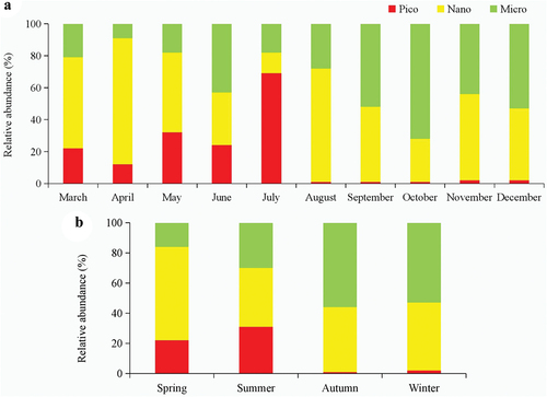
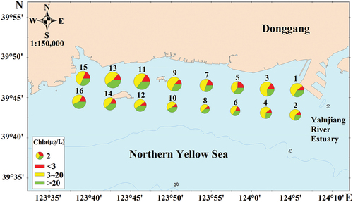
The picophytoplankton proportions showed a trend of first rising and then falling, and the highest proportion was in summer and lower proportions (<2%) were found in autumn and winter (Figure 3b). The trend of nanophytoplankton was relatively steady in all four seasons, the highest proportion was in spring. The proportions of microphytoplankton showed a gradual upward trend from spring to winter. The proportions of nanophytoplankton and microphytoplankton were similar in autumn and winter. Picophytoplankton and nanophytoplankton formed the dominant community in spring and summer, and the sum of picophytoplankton and nanophytoplankton proportions was greater than 74%. In autumn and winter, the sum of picophytoplankton and nanophytoplankton proportions were similar to microphytoplankton. In general, the biomass of phytoplankton near the shore of the estuary (Stations 1, 3, 5, 7, 9, 11, 13, and 15) was higher than in the offshore of the estuary (Figure 4). The biomass of phytoplankton in the west of the estuary was higher than in other stations.

Figure 4. Distribution of different size-fractioned phytoplankton biomass in Yalu River Estuary, China.

Water quality parameters

The mean values of the various seasonal environmental parameters were shown in Table 2. The temperature was highest in summer, followed by autumn and spring, and lowest in winter. The nitrite and ammonia nitrogen gradually increased. The nutrient concentrations were higher in autumn and winter than in spring and summer.

Table 2. Means of the various environmental parameters from each cruise measured in the Yalu River Estuary, China, in 2020.

Season variable	Spring average (±SD)	Summer average（±SD）	Fall average（±SD）	Winter average（±SD）	Annual average（±SD）
Dep (m)	5.51±2.09	6.24±1.96	5.18±1.48	5.66±1.55	5.65±0.30
T (℃)	10.45±0.23	23.33±0.46	16.86±0.09	4.33±1.07	13.74±6.36
SST	26.92±0.62	27.37±0.42	24.92±0.81	27.22±0.70	26.61±0.84
pH	7.81±0.04	7.65±0.09	7.97±0.02	7.70±0.11	7.78±0.11
DO (mg/L)	9.22±0.17	7.95±0.18	9.43±0.10	10.60±0.32	9.30±0.72
TN (mg/L)	0.329±0.048	0.250±0.036	0.358±0.055	0.501±0.129	0.359±0.062
TP (mg/L)	0.009±0.001	0.244±0.064	0.186±0.017	0.028±0.006	0.117±0.016
COD (mg/L)	1.36±0.31	1.11±0.19	1.24±0.10	1.04±0.41	1.19±0.11
DIP (mg/L)	0.003±0.001	0.011±0.004	0.015±0.003	0.02±0.006	0.012±0.003
SiO3 (mg/L)	0.16±0.030	0.936±0.183	0.958±0.144	0.952±0.154	0.752±0.091
NO2 (mg/L)	0.005±0.001	0.010±0.002	0.026±0.001	0.032±0.001	0.018±0.001
NO3 (mg/L)	0.178±0.023	0.197±0.047	0.338±0.050	0.271±0.040	0.246±0.030
NH4 (mg/L)	0.043±0.019	0.070±0.013	0.080±0.016	0.097±0.031	0.073±0.014
DIN (mg/L)	0.227±0.035	0.277±0.060	0.444±0.064	0.400±0.065	0.337±0.042
N/P	119.93±63.520	60.04±28.45	47.22±13.66	22.36±5.07	62.39±28.77

The principal component analysis (PCA) sequence diagram of environmental factors at 16 stations in all four seasons showed the spatial distribution pattern of the gradient changes of environmental factors in the Yalu River Estuary (Figure 5). In spring, pH, TN, and SiO₃ made significant environmental contributions in the east of the estuary (Stations 1, 2, 3, and 4), and TN was an important environmental factor in the east of the estuary. In the middle part of the estuary (Stations 7, 8, 9, and 10), Dep and N/P had a close correlation with water quality. In the west of the estuary (Stations 13, 14, 15, and 16), TP and DIP made significant environmental contributions. The values of N/P gradually decreased from right to left along the PC1 axis, while the value of SiO₃ and COD gradually increased from bottom to top along the PC2 axis. The environmental factors of Stations 1, 13, and 15 were quite different from the other stations: the TN, SiO₃, DIN, and N/P of Station 1 were the highest among all stations, COD values at Station 13 were the highest among all stations. The water temperature at Station 15 was the highest among all stations (Figure 5a). In summer, the aquatic systems of the entire estuary were significantly affected by many environmental factors, such Dep, DO, SST, pH, TP, COD, DIP, and SiO₃. All environmental factors made significant environmental contributions in the east of the estuary. N/P gradually decreased from right to left along the PC1 axis, and Dep gradually decreased from top to bottom along the PC2 axis. Among them, Stations 1, 4, and 15 were quite different from other stations. SST and DO values of Station 1 were the lowest among all stations, while TN and DIP values were the highest among all stations. TP, DIP and SiO₃ values at Station 4 were the lowest among all stations. At Station 15, Dep and pH were the lowest among all stations, while SST, TP, COD, SiO₃, and DIN were the highest among all stations (Figure 5b). In autumn, DIN, TN, SiO₃, and DIP were significant environmental factors in the east of the estuary, and DO, N/P and Dep were important environmental factors in the middle part of the estuary. Dep and N/P values gradually decreased from right to left along the PC1 axis, and SST values gradually increased from bottom to top along the PC2 axis. Among them, Stations 1, 2, 9, 11, and 15 were quite different from other stations (Figure 5c). In winter, the aquatic systems of the eastern estuary were mainly affected by TN, TP, SiO₃, DO, COD, and N/P. All environmental factors made significant environmental contributions in the west of the estuary. The TP and DIN values gradually increased from left to right along the PC1 axis, while the N/P value gradually increased from bottom to top along the PC2 axis. Station 1 was obviously different from other stations. Dep, T, SST, and N/P were the lowest, while pH, TN, TP, COD, DIP, SiO₃, and DIN were the highest in Station 1(Figure 5d). Comprehensive analysis throughout the year, that is, station average (the average value of the content of relevant environmental factors from March to December corresponding to the 16 stations), the aquatic systems of the eastern estuary were mainly affected by TN, DIN, DIP, SiO₃, COD, and TP. No environmental factors made significant environmental contributions in the west of the estuary, and DO, N/P, pH, and Dep were important environmental factors in the middle part of the estuary. N/P values gradually decreased from right to left along the PC1 axis, and DIP values gradually increased from bottom to top along the PC2 axis (Figure 5e).

Figure 5. PCA analysis of correlation between stations/months and environmental factors in Yalu River Estuary, China. (a: spring; b: summer; c: autumn; d: winter; e: station average; f: monthly average; 1–16 in Fig (A-E) represent 16 stations;3–12 in Fig (F) represent March to December).

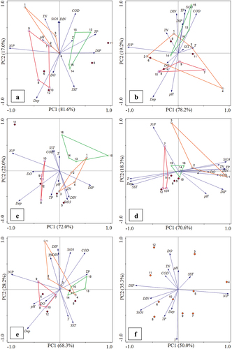
The principal component analysis sequence diagram of the average of environmental factors at 16 stations in each month have obviously patch distribution characteristics (monthly average, that is, the average value of the relevant environmental factors of 16 stations in each month from March to December), and there were significant differences between the Yalu River and Dayang River estuary at both ends and the central sea area. Some environmental factors in March, April, July, and November were quite different from those in other months (Figure 5f). In March, TP, DIP, SiO₃, and DIN values were the lowest of the whole year. In April, COD and DIP values were the lowest of the whole year, while N/P values were the highest of the whole year. In July, the DO value was the lowest and the T value was the highest of the whole year. In November, the N/P value was the lowest and pH, COD, DIP, and DIN values were the highest of the whole year.

Correlation between size fraction of phytoplankton and environmental factors

Correlation between phytoplankton and environmental factors at each station in four seasons

The distribution of different size-fraction phytoplankton in the 16 estuary stations was affected by many environmental factors (Table 3, Figure 6). The results showed that SST, COD, T and Dep significantly affected the distribution of total phytoplankton (P < 0.05). SST, COD and T had positive effects and Dep harmed the distribution of the entire community. The distribution of the picophytoplankton community was positively affected by SST and COD, and negatively affected by Dep and pH. The nanophytoplankton community was positively affected by the T and negatively affected by Dep. The microphytoplankton community was positively affected by SST, COD and T, and negatively affected by Dep (Figure 6e).

Figure 6. RDA analysis of correlation between phytoplankton and environmental factors in Yalu River Estuary, China. (a: spring; b: summer; c: autumn; d: winter; e: station average (the average value of the content of relevant environmental factors and the number of phytoplankton sequences from March to December corresponding to the 16 stations); f: monthly average (the average value of the relevant environmental factors and microalgae sequence numbers of 16 stations in each month from March to December); Blue arrow: phytoplankton; red arrow: each environmental factor). The cosine of the angle between the red arrow and the blue arrow represents the correlation between the environmental variable and the phytoplankton biomass. Explanatory quantity and significance test of environmental factors are shown in Table 3. The abbreviation codes of phytoplankton species are shown in Table S1. Means of the various environmental parameters from each month measured in the Yalu River Estuary, China, in 2020 are shown in Table S2.

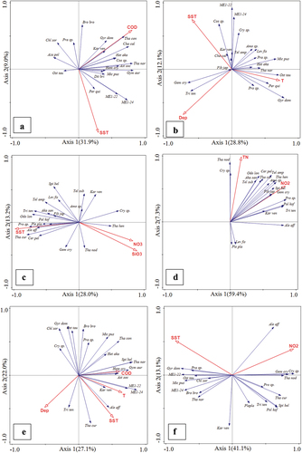
Table 3. Explanatory quantity and significance test of environmental factors.

Time	Grain size community	Environmental factors	Interpretation quantity	pseudo-F	P
Spring	Total	COD	24	4.4	0.002
		SST	16.9	3.7	0.002
	Pico-	SST	23	4.2	0.014
		Dep	34.1	10.4	0.002
	Nano-	COD	28.8	5.7	0.002
		TN	14.9	3.4	0.018
	Micro-	COD	50.6	14.3	0.002
		N/P	22.5	10.9	0.002
		SST	5.5	3.1	0.040
Summer	Total	Dep	21.9	3.9	0.004
		SST	18	3.9	0.002
		T	8.7	2	0.032
	Pico-	Dep	25.7	4.8	0.008
		SST	22.6	5.7	0.010
	Nano-	T	20.5	3.6	0.010
	Micro-	Dep	34.9	7.5	0.004
		SST	25.1	8.1	0.002
Autumn	Total	SST	27.2	5.2	0.002
		SiO3	13.4	2.9	0.012
		NO3	10.8	2.7	0.026
	Nano-	TN	25.8	4.9	0.026
		DO	15.6	3.5	0.048
		DIP	17.9	5.3	0.02
	Micro-	SiO3	32.2	6.7	0.002
		DIP	12.4	2.9	0.032
Winter	Total	NO2	44	11	0.002
		TN	22.8	8.9	0.006
	Nano-	TP	62.9	23.7	0.002
		TN	8.7	4	0.014
	Micro-	NO2	43.3	10.7	0.002
		TN	23.7	9.4	0.006
Station average	Total	SST	18.2	3.1	0.006
		Dep	17.9	3.6	0.002
		T	12.2	2.8	0.006
		COD	10.7	2.9	0.002
	Pico-	SST	23.7	4.4	0.008
		pH	20.6	4.8	0.008
		COD	13.4	3.8	0.012
		Dep	8.2	2.7	0.034
	Nano-	T	17.9	3.1	0.010
		Dep	22.8	5	0.002
	Micro-	Dep	23.9	4.4	0.006
		SST	21.9	5.3	0.002
		COD	11.8	3.3	0.006
		T	10.6	3.7	0.006
Monthly average	Total	NO2	33.6	4.1	0.010
		SST	14.7	2.7	0.04
	Pico-	NO2	41.5	5.7	0.034
	Nano-	NO2	38.8	5.1	0.012
	Micro-	SST	43.7	6.2	0.004
		NO2	15.2	2.6	0.042

In spring, a significant positive correlation was observed between total phytoplankton and COD and SST. The picophytoplankton community was significantly positively affected by SST and extremely significantly negatively affected by Dep. Nanophytoplankton was positively affected by TN and COD. The microphytoplankton community was negatively affected by SST and N/P, COD had a positively significant influence on microphytoplankton community (Figure 6a). In summer, SST, T, and Dep had positive and negative influences, respectively, on all phytoplankton communities. Among them, picophytoplankton and microphytoplankton were significantly positively affected by SST and negatively affected by Dep. Nanophytoplankton were positively affected by T(Figure 6b). In autumn, SST, NO₃, and SiO₃ had a significant influence on total phytoplankton communities. SST showed a positive effect on total phytoplankton communities; in contrast, NO₃ and SiO₃ showed a negative effect. Nanophytoplankton was negatively affected by TN and DIP, and microphytoplankton were negatively affected by DIP and NO_3， while picophytoplankton had no significant correlation to environmental factors (Figure 6c). In winter, TN and NO₂ had positively significant influences on total phytoplankton communities, especially microphytoplankton. Nanophytoplankton was positively affected by TP and TN (Figure 6d).

Correlation between phytoplankton and environmental factors at each station in four seasons

In 2020, the environmental factor that significantly controlled the total community structure of phytoplankton were NO₂ and SST (P < 0.05), but the direction controlling the evolution of the whole community varied in the time series (Table 3, Figure 6f). Among them, the community structure of picophytoplankton and nanophytoplankton was negatively affected by NO₂. The community structure of microphytoplankton was positively affected by NO₂ and SST.

The dominant species with different particle sizes were also related to different environmental factors. In the picophytoplankton community, O. tauri and M. pusilla were negatively affected by NO₂. In the nanophytoplankton community, K. veneficum and T. nordenskioeldii were negatively affected by NO₂, while Cryptomonadales sp. was positively affected by NO₂. In microphytoplankton, A. affine and T. curviseriata were positively affected by NO₂ and negatively affected by SST, while G. dominans was positively affected by SST and negatively affected by NO₂.

Discussion

Feasibility of molecular identification method for phytoplankton

The survey found that K. veneficum was detected with higher frequency and that this species had the greatest dominance in spring, summer, and autumn. A. affine was the most dominant species in winter. The routine water quality environmental monitoring method of morphological microscopy was generally used to identify the phytoplankton. In this survey, morphological microscopy identified Skeletonema sp. as the dominant species, but molecular identification found the proportion of Skeletonema sp. to be only 0.46% of the total biomass. Jiang et al. found that Pseudonitzschia pungzns, Skeletonema costatum, Chaetoceros affinis, Chaetoceros curvisetus, and Noctiluca scintillans were the dominant species by morphological microscopy in Yalu River Estuary from 2011 to 2015 (Jiang et al. 2017). The results revealed that morphological microscopy and molecular identification yielded quite different results on phytoplankton identification. In 2019, Song et al. conducted a study on the northern waters of the Yellow Sea using the high-throughput sequencing method (Song et al. 2021). The results showed that K. veneficum was the dominant species, with a higher ecological niche in spring, summer, and autumn, which was consistent with the results of this study. It can be seen that morphological identification usually missed smaller phytoplankton (<10 μm), which also proved the scientific and repeatable molecular identification method. Morphological identification can only obtain the density and volume of large-sized phytoplankton, while molecular identification can obtain the sequence number and biomass data of full-sized phytoplankton OTUs. For shellfish feeding nutrition, bait biomass was more scientifically meaningful than density. Many molecular identification methods and tools – such as amplification region, primer, PCR process, amplification efficiency, length analysis, and databases (Song et al. 2018, 2019c) – are now used, and compared to the traditional morphological microscopic examination, which have improved the discovery of species diversity by an order of magnitude. The scientific method of molecular identification promotes the discovery of picophytoplankton and nanophytoplankton, and avoids potential subjective errors in morphological identification. With the development of high-throughput sequencing technology, many technical parameters have improved, such as increased sequencing throughput, longer fragment sequencing, and more sophisticated databases. This investigation used the molecular identification method to discover the phytoplankton biomass dominant species, Karlodinium veneficum, which had not been found by the morphological identification method before, showed the accuracy and reliability of the molecular identification method.

Environmental factors affecting the size structure of phytoplankton on the time dimension

Near the Yalu River Estuary in the northern Yellow Sea (Station 10, not investigated in winter), the largest proportions of nanophytoplankton and microphytoplankton biomass appeared in the spring (May) and autumn (October) in 2019 (Song et al. 2021). The results were consistent with the results of this study. The proportion of picophytoplankton was the largest in the summer (August) in 2019, except that nanophytoplankton biomass was found to be the greatest in summer 2020. The difference may be related to the change in the dominant species.

In summer 2019, near the Yalu River Estuary (Station 10), the first dominant species was Mamiella gilva, and the second dominant species was K. veneficum. In August 2020, the first dominant species in the waters near the Yalu River Estuary was K. veneficum with a dominance of 0.49, but in July 2020 the first dominant species was the O. tauri, which was picophytoplankton with a dominance of 0.41, while K. veneficum was only 0.03. The changes of dominant species were caused by different investigation time and changes of environmental factors. In July 2020, DIN was 0.084 mg/L and DIP was 0.001 mg/L, while in August 2020, DIN was 0.543 mg/L and DIP was 0.016 mg/L. The nutrients were significantly increased and the dominant species was changed from picophytoplankton to nanophytoplankton. Similarly, in August 2019, DIN content in the sea area near Yalu River estuary was 0.051 mg/L and DIP was 0.002 mg/L, similar to July 2020, it was found that high content of inorganic N and P could promote the growth of phytoplankton in large-grain scale (Yunev et al. 2007; Harrison et al. 1990; Jiao and Wang 1994).

In the whole year, the biomass of picophytoplankton gradually increased from spring to summer, while it tended to zero in autumn and winter. Nanophytoplankton tended to decline gradually, while microphytoplankton tended to rise gradually. The change of picophytoplankton may be related to the first dominant species of the picophytoplankton community – Ostreococcus tauri. Song Lun et al. found that the biomass of O. tauri was higher in spring and summer, but not in autumn and winter, which may be due to the influence of temperature on the reproduction of the algae in Liaodong Bay in 2014 (Song et al. 2018). In the time dimension (Monthly average), nanophytoplankton was negatively affected by NO₂, and microphytoplankton was positively affected by NO₂. NO₂ gradually increased from spring to winter in the Yalu River Estuary in 2020, so the biomass of nanophytoplankton gradually decreased, and the biomass of microphytoplankton gradually increased. Although NO₂ accounted for the lowest proportion of DIN, it had a great influence on the evolution of phytoplankton communities in winter and inter-lunar phytoplankton community structures, and the reason may be that as a limiting factor, the fluctuation of its concentration will significantly affect the proportion of the main dominant phytoplankton.

Environmental factors affecting the size structure of phytoplankton on the spatial dimension

On the spatial dimension (Station average), the spatial distribution of the total phytoplankton community was positively affected by SST in spring, summer, and autumn, while in winter, TN and NO₂ had positively significant influences on total phytoplankton communities, especially microphytoplankton. The structure of the picophytoplankton community was positively affected by SST and negatively affected by Dep in spring and summer, but had no significant association with environmental factors in autumn and winter, it should be noted that the seawater depth (Dep) parameter analyzed in this article simply refers to the distance (dimension). Nanophytoplankton had positively affected by TN in spring, autumn and winter, and was positively affected by T in the summer. The community structure of microphytoplankton was positively affected by COD in spring, but negatively by DIP and SiO₃ in autumn. SST and TN showed positive effects on the microphytoplankton community in summer and winter, respectively.

The east and west sides of the Yalu River Estuary comprise the Yalu River and Dayang River estuaries, respectively. Because of the inflow of freshwater, SST was relatively low on the eastern and western sides of the Yalu River Estuary, while it was very high in the middle part. SST had a great influence on the community structure and distribution of microphytoplankton and picophytoplankton. With the increase in SST, the proportions of microphytoplankton and picophytoplankton gradually increased in the Yalu River Estuary.

Environmental factors in the water body have a great influence on the growth and reproduction of phytoplankton, and then control the evolution of their populations and communities in space and time. In spring, abundant light, suitable temperature and accumulation of nutrients brought favorable conditions for the growth of phytoplankton, which made the small-sized phytoplankton with r-countermeasures as the main factor propagate rapidly (Song et al. 2015); In summer, most nutrients in seawater were consumed by phytoplankton, the nutrients were not replenished from land sources in time, and the growth of phytoplankton slowed down; In autumn, due to the nutrient consumption was greater than the replenishment, the small-sized phytoplankton dominated by r-countermeasure was gradually replaced by the large-sized phytoplankton of k-countermeasure, and the community gradually recovered to the equilibrium point. In winter, the community was mainly affected by the water temperature, so the feedback regulation was mainly completed by the large-sized phytoplankton of k-countermeasure. Of course, the evolution of phytoplankton granular structure is not only affected by the upward effect of environmental factors, but also by the downward effect of the massive feeding of shellfish and zooplankton (Grover 1989). In recent decades, filter-feeding shellfish such as Ruditapes philippinarum has been mainly cultivated in this sea area, and there was a great demand for natural bait phytoplankton. With the reduction of terrestrial nitrogen and phosphorus, the inorganic nutrients in the sea area gradually decrease, which may exacerbate the trend of miniaturization of phytoplankton. Hoping to get the attention of relevant parties (Song et al. 2019c).

The main dominant species and their ecological toxicity

In recent years, the frequency of red tides (blooms) has increased in Chinese coastal waters. K. veneficum is a toxic dinoflagellate and contains hemolysin, fish toxins, and cytotoxins, Cytotoxins are polar lipids (karlotoxins) and can be divided into KmTx1 and KmTx2 (Deeds and Place 2006). Some studies have indicated that K. veneficum caused abnormal embryonic development in mussels and has an effect on the survival of cod juveniles (Nielsen 1993) and golden-headed Sparus, especially in the hatching of fertilized eggs and the survival of young sea bass (Zhou et al. 2011). Adolf found that the toxin of K. veneficum could inhibit the growth of Fibrocapsa japonica and Storeatula major (Adolf et al. 2006a). The filtrate of K. veneficum (an algae-free cell) in the late exponential growth stage could inhibit the growth of Prorocentrum donghaiense, but Prorocentrum donghaiense filtrate did not affect the growth of K. veneficum (Wang et al. 2019). The Karlodinium sp. can inhibit the growth of various phytoplankton such as Akashiwo sanguinea, Prorocentrum micans, Scrippsiella acuminata, Phaeocystis globosa, and Rhodomonas salina, and the inhibition rate has been found to be positively correlated with the cell density of K. veneficum. And the inhibition rate is positively correlated with the cell density of K. veneficum. The higher the abundance of K. veneficum, the higher the inhibition rate of R. salina. The inhibition rates of the K. veneficum with an initial density of 2000 cells·mL⁻¹ to R. salina were 18%, 36% and 53% under low, medium and high nutritional conditions, respectively, and the inhibition rates of K. veneficum with an initial density of 8000 cells·mL⁻¹ to R. salina were 30%, 48%, and 64% under low, medium, and high nutrient conditions, respectively (Shi 2018). In addition, A. sanguinea, S. trochoidea, P. globosa, and R. salina had a significant effect on the growth of K. veneficum. Among them, the growth of K. veneficum J×24 co-cultured with R. salina could be promoted by up to 3.4 times (Yan 2019). Therefore, it is obvious that the growth advantage of K. veneficum. K. veneficum affects the succession of a phytoplankton community in natural seawater, and its influence on phytoplankton varies. In different algae, K. veneficum could promote or hinder their original succession, and even changed its direction (Wang, Yan, and Zhou 2015). The toxic mechanism and toxic pathway of K. veneficum has been found to be different in different organisms (Adolf, Bachvaroff, and Place 2009).

Adolf reported that the outbreak rate of K. veneficum red tides was higher in eutrophic water bodies (Adolf, Bachvaroff, and Place 2009), such as in hybrid striped perch aquaculture fisheries (Deeds et al. 2002), South Carolina Reserve (Kempton et al. 2002), Corsica River, a tributary of Chesapeake Bay, and in other areas (Hall et al. 2008). In recent years, blooms of K. veneficum have also often occurred in eutrophic waters in China. In April 2011, during a bloom of K. veneficum, the concentrations of dissolved inorganic nitrogen, silicate, and phosphate were abnormally higher than in the same period of the previous year in Sanggou Bay (Zhang et al. 2012). In this study, the levels of nutrients were higher in spring and summer in the Yalu River Estuary, and the biomass of K. veneficum was relatively greater.

Cranford et al. (Cranford et al. 2008) found that bivalve mollusks were easy to feed on nanophytoplankton, K. veneficum is nanophytoplankton, so Ruditapes philippinarum like to eat it. However, nutrients – as the basis for the growth of phytoplankton – also played a role in regulating the toxicity of the dominant species K. veneficum in the Yalu River Estuary. Studies have found that high concentrations of nitrogen have a significant effect on the toxicity of K. veneficum, which gradually weakens with a decrease in nitrogen concentrations. This indicates that high concentrations of nitrogen promote the release of toxic substances (Glibert and Terlizzi 1999), posing a serious threat to R. philippinarum breeding. The aquaculture area of this fishery was 45,000 ha and the annual output was about 240,000 tons, accounting for 20% of the total output of R. philippinarum in Liaoning Province and 6% in China. The health and safety of shellfish should be taken seriously (Song et al. 2016b, 2019b).

Conclusion

1. The dominant species in the Yalu River Estuary was the nanophytoplankton species K. veneficum, which was discovered for the first time.

2. In Yalu River Estuary, the biomass ratio of picophytoplankton, nanophytoplankton, and microphytoplankton was 20:63:17 in spring, 30:44:26 in summer, 1:38:61 in autumn, and 2:45:53 in winter, respectively. The biomass of picophytoplankton and nanophytoplankton was greater in spring and summer. The biomass of microphytoplankton was greater in autumn and winter. This result was the first discovery.

3. The biomass of Dinophyta was the greatest, followed by Bacillariophyta, and the occurrence frequency and biomass of Dictyochophyta, Chrysophyta, and Cryptophyta were lower, which subverted the conclusion of morphological identification: diatoms were Bacillariophyta, and Dinophyta was the second.

4. On the spatial dimension (Station average), the environmental factors that significantly controlled the evolution of phytoplankton community structure on the spatial scale were COD, Dep, T, SST. COD, T, SST had a positive impact on total phytoplankton communities, and Dep had a negative impact. Among them, the distribution of the picophytoplankton community was positively affected by SST and COD, and negatively affected by Dep and pH. The nanophytoplankton community was positively affected by T and negatively affected by Dep. The microphytoplankton community was positively affected by SST, COD and T, and negatively affected by Dep.

5. In the time dimension (Monthly average), the environmental factor that significantly controlled the phytoplankton community structure were NO₂ and SST , but the direction of the evolution of the entire community was different in the time series. Among them, the community structure of picophytoplankton and nanophytoplankton was negatively affected by NO₂. The community structure of microphytoplankton was positively affected by NO₂ and SST.

Acknowledgments

Thank colleagues for their assistance in collecting samples.

Disclosure statement

No potential conflict of interest was reported by the author(s).

Additional information

Funding

This research was funded by outstanding young scientific and technological personnel of Dalian (2019RJ09); The Applied Basic Research Plan of Liaoning Province (2022010280); Liaoning revitalization talents program (XLYC1907109); Modern Agro-industry Technology Research System (CARS-49); Liaoning Marine and fishery scientific research projects (201828, 201824).

References

- Adame, M. F., J. Alcocer, and E. Escobar. 2008. “Size-Fractionated Phytoplankton Biomass and Its Implications for the Dynamics of an Oligotrophic Tropical Lake.” Freshwater Biology 53 (1): 1–15.
- Adolf, J., T. Bachvaroff, D. Krupatkina, H. Nonogaki, P. Brown, A. Lewitus, H. Harvey, and A. Place. 2006a. “Species Specificity and Potential Roles of Karlodinium Micrum Toxin.” South African Journal of Marine Science 28 (2): 415–419. doi:10.2989/18142320609504189.
- Adolf, J. E., T. Bachvaroff, and A. R. Place. 2009. “Can Cryptophyte Abundance Trigger Toxic Karlodinium Veneficum Blooms in Eutrophic Estuaries?” Harmful Algae 8 (1): 119–128. doi:10.1016/j.hal.2008.08.003.
- Claustre, H., M. Babin, D. Merien, J. Ras, L. Prieur, and S. Dallot. 2005. “Toward a Taxon-Specific Parameterization of Bio-Optical Models of Primary Production: A Case Study in the North Atlantic.” Journal of Geophysical Research Atmospheres 110: C07S12.
- Cranford, P. J., W. Li, Ø. Strand, and T. Strohmeier. 2008. “Phytoplankton Depletion by Mussel Aquaculture: High Resolution Mapping, Ecosystem Modeling and Potential Indicators of Ecological Carrying Capacity.” ICES CM Doc 2008/ H: 12. International Council for the Exploration of the Sea, Copenhagen. http://ices.dk/sites/pub/CM%20Doccuments/CM-2008/H/H1208.pdf
- Deeds, J. R., and A. R. Place. 2006. “Sterol-Specific Membrane Interactions with the Toxins from Karlodinium Micrum (Dinophyceae) —strategy for Self-Protection?” African Journal of Marine Science 28 (2): 421–425. doi:10.2989/18142320609504190.
- Deeds, J. R., D. E. Terlizzi, J. Adolf, D. K. Stoecker, and A. R. Place. 2002. “Toxic Activity from Cultures of Karlodinium Micrum (=Gyrodinium Galatheanum) (Dinophyceae)—a Dinoflagellate Associated with Fish Mortalities in an Estuarine Aquaculture Facility.” Harmful Algae 1 (2): 169–189. doi:10.1016/S1568-9883(02)00027-6.
- Faria, D. G., M. D. Lee, J. B. Lee, J. Lee, M. Chang, S. Youn, Y. Suh, and J. S. Ki. 2014. “Molecular Diversity of Phytoplankton in the East China Sea Around Jeju Island (Korea), Unraveled by Pyrosequencing.” Journal of Oceanography 70 (1): 11–23. doi:10.1007/s10872-013-0208-2.
- Fu, R., and J. Gong. 2017. “Single Cell Analysis Linking Ribosomal (R)DNA and rRna Copy Numbers to Cell Size and Growth Rate Provides Insights into Molecular Protistan Ecology.” The Journal of Eukaryotic Microbiology 64 (6): 885–896. doi:10.1111/jeu.12425.
- Glibert, P. M., and D. E. Terlizzi. 1999. “Cooccurrence of Elevated Urea Levels and Dinoflagellate Blooms in Temperate Estuarine Aquaculture Ponds.” Applied & Environmental Microbiology 65: 5594.
- Godhe, A., M. E. Asplund, K. Harnstrom, V. Saravanan, A. Tyagi, and I. Karunasagar. 2008. “Quantification of Diatom and Dinoflagellate Biomasses in Coastal Marine Seawater Samples by Real-Time PCR.” Applied and Environmental Microbiology 74 (23): 7174–7182. doi:10.1128/AEM.01298-08.
- Grover, J.P. 1989. “Influence of Cell Shape and Size on Algal Competitive Ability [J].” Journal of Phycology 25 (2): 402–405. doi:10.1111/j.1529-8817.1989.tb00138.x.
- Gu, B. 2014. Molecular Ecology Research of the Brown Tide (aureococcus anophagefferens) in Qinhuangdao Scallop Culture Area. Qing Dao: Ocean University of China.
- Hall, N. S., R. W. Litaker, E. Fensin, J. E. Adolf, H. A. Bowers, A. R. Place, and H. W. Paerl. 2008. “Environmental Factors Contributing to the Development and Demise of a Toxic Dinoflagellate (Karlodinium Veneficum) Bloom in a Shallow, Eutrophic, Lagoonal Estuary.” Estuaries & Coasts 31 (2): 402–418. doi:10.1007/s12237-008-9035-x.
- Harrison, P. J., M. H. Hu, Y. P. Yang, and X. Lu. 1990. “Phosphate Limitation in Estuarine and Coastal Waters of China.” Journal of Experimental Marine Biology and Ecology 140 (1/2): 79–87.
- Jiang, X. J. 2009. Analysis of Picoplankton Abundance and Study of Genetic Diversity of Microeukaryotes in the in the North Yellow Sea. Qing Dao: Ocean University of China.
- Jiang, S., Y. Z. Chen, G. R. Cao, H. Q. Chen, and X. G. Liu. 2017. “Phytoplankton Community in Donggang Red-Tide-Monitoring Area, Yalujiang River Estuary.” Fisheries Science 36 (05): 617–622.
- Jiao, N. Z., and R. Wang. 1994. “Size Structures of Microplankton Biomass and Production in Jiaozhou Bay, China.” Journal of Plankton Research 16 (12): 1609–1625.
- Kempton, J. W., A. J. Lewitus, J. R. Deeds, J. McHugh Law, and A. R. Place. 2002. “Toxicity of Karlodinium Micrum (Dinophyceae) Associated with a Fish Kill in a South Carolina Brackish Retention Pond.” Harmful Algae 1 (2): 233–241. doi:10.1016/S1568-9883(02)00015-X.
- Lafond, M., B. Pinel-Alloul, and P. Ross. 1990. “Biomass and Photosynthesis of Size-Fractionated Phytoplankton in Canadian Shield Lakes.” Hydrobiologia 196 (1): 25–38. doi:10.1007/BF00008890.
- Legendr, L. 1999. “Environmental Fate of Biogenic Carbon in Lakes.” Japanese Journal of Limnology 60 (1): 1–10. doi:10.3739/rikusui.60.1.
- Liu, R. Y. 2008. Checklist of Marine Biota of China Seas 301–870. Bei Jing: Science Press.
- Magoč, T., and S. L. Salzberg. 2011. “Flash: Fast Length Adjustment of Short Reads to Improve Genome Assemblies.” Bioinformatics 27 (21): 2957–2963. doi:10.1093/bioinformatics/btr507.
- Melack, J. M. 1976. “Primary Productivity and Fish Yields in Tropical Lakes.” Transactions of the American Fisheries Society 105 (5): 575–580. doi:10.1577/1548-8659(1976)105<575:PPAFYI>2.0.CO;2.
- Naselli-Flores, L., and R. Barone. 2003. “Steady–state Assemblages in a Mediterranean Hypertrophic Reservoir. The Role of Microcystis Ecomorphological Variability in Maintaining an Apparent Equilibrium.” Hydrobiologia 502 (1–3): 133–143. doi:10.1023/B:HYDR.0000004276.11436.40.
- Nielsen, M. V. 1993. “Toxic Effect of the Marine Dinoflagellate Gymnodinium Galatheanum on Juvenile Cod Gadusmorhua.” Marine Ecology Progress Series 95 (3): 273–277. doi:10.3354/meps095273.
- Prokopowich, C. D., T. R. Gregory, and T. J. Crease. 2003. “The Correlation Between rDna Copy Number and Genome Size in Eukaryotes.” Genome 46 (1): 48–50. doi:10.1139/g02-103.
- Shi, J. 2018. Allelopathic Effects and Its Ecological Significance of karlodinium Veneficum on Co-Occuring Phytoplankton. Jinan University. doi:10.27167/d.cnki.gjinu.2018.000191.
- Song, L., X. D. Bi, J. Fu, G. J. Song, J. H. Du, Y. Liu, and S. X. Liu. 2021. “Characteristics of Eukaryotic Microalgae and Their Environmental Correlation in the Northern Yellow Sea.” China Environmental Science 41 (03): 1336–1344.
- Song, L., X. D. Bi, G. J. Song, J. Du, J. H. Wu, Z. S. Wang, and C. K. Hu. 2020. “Size-Fractionated Eukaryotic Microalgae and Its Influencing Factors Dachangshan Island and Its Adjacent Waters.” China Environmental Science 40: 2627–2634.
- Song, L., G. J. Song, N. B. Wang, H. B. Zhao, J. Tian, S. Yang, and J. Du. 2015. “The Stress Response of Net Phytoplankton Biomass Size Structure in Liaodong Bay.“ China Environmental Science 35 (09): 2764–2771.
- Song, L., J. Wu, J. Du, N. Li, G. J. Song, K. Wang, M. Sun, and P. Wang. 2019b. “The Characteristics and Distribution of Eukaryotic Phytoplankton Community in Liaodong Bay, China.” Ocean Science Journal 54 (2): 183–203. doi:10.1007/s12601-019-0007-9.
- Song, L., J. Wu, J. Du, N. Li, K. Wang, and P. Wang. 2019a. “Comparison of Two Methods to Assess the Size-Structure of Phytoplankton Assemblages in Liaodong Bay, China.” Journal of Ocean University of China 18 (5): 1207–1215. doi:10.1007/s11802-019-3960-0.
- Song, L., J. Wu, N. Li, J. Du, S. Yang, and P. Wang. 2018. “The Temporal and Spatial Distribution of Potential Brown Tide Species and Correlation Analysis with Environmental Factors in Liaodong Bay.” China Environmental Science 38 (8): 3060–3071.
- Song, L., J. Wu, N. Li, M. Sun, J. Du, and P. Wang. 2019c. “Quality Control Analysis of Eukaryotic Microalga Diversity Based on High-Throughput Sequencing in Liaodong Bay.” Fisheries Science 38 (06): 804–812.
- Song, L., J. Wu, W. D. Liu, Y. Song, and N. Wang. 2016b. “Diversity of Marine Nanophytoplankton and Picophytoplankton in Changxing Island Offshore Waters of Bohai.” Sea Research of Environmental Sciences 29 (11): 1635–1642.
- Song, L., J. Wu, Y. G. Song, W. D. Liu, and G. J. Yang. 2017. “Distribution of Brown Tide Species Aureococcus Anophagefferens in Liaodong Bay.” Research of Environmental Sciences 30 (4): 537–544.
- Song, L., G. J. Yang, N. B. Wang, and X. Q. Lu. 2016a. “Relationship Between Environmental Factors and Plankton in the Bayuquan Port, Liaodong Bay, China: A Five-Year Study.” Journal of Oceanology and Limnology 34 (4): 654–671.
- Song, G. J., X. Zhang, L. Song, N. B. Wang, and A. Li. 2013. “Aquaculture Carrying Capacity of Manila Clam Ruditapes Philippenarum at Shallow Sea Area in Yalu River Estuary.” Fisheries Science 32 (01): 36–40.
- Stoeck, T., D. Bass, and M. Nebel. 2010. “Multiple Marker Parallel Tag Environmental DNA Sequencing Reveals a Highly Complex Eukaryotic Community in Marine Anoxic Water.” Molecular Ecology 19: 21–31.
- Temponeras, M., J. Kristiansen, and M. Moustaka-Gouni. 2000. “Seasonal Variation in Phytoplankton Composition and Physical-Chemical Features of the Shallow Lake Doirani, Macedonia, Greece.” Hydrobiologia 424 (1): 109–122. doi:10.1023/A:1003909229980.
- Wang, R., W. W. Huang, J. J. Wu, L. L. Chan, and J. T. Wang. 2019. “Allelopathic Interaction of Two Dinoflagellates: Karlodinium Veneficum and Prorocentrum Donghaiense.” Oceanologia Et Limnologia Sinica 50 (04): 858–863.
- Wang, Y., and S. X. Liu. 2018. “Size-Fractionated Chlorophyll-A and Its Relationship with Environmental Factors in Adjacent Water of the Yalu River Estuary in Summer.” Marine Environmental Science 37 (06): 879–887.
- Wang, C. C., T. Yan, and M. J. Zhou 2015. A Preliminary Study of the Toxicity and Mechanism of karlodinium Veneficum to Marine Organisms. Marine Envionmental Science 34 (06): 801–805+818. doi:10.13634/j.cnki.mes.2015.06.001.
- Xu, X., Z. Yu, F. Cheng, L. He, X. Cao, and X. Song. 2017. “Molecular Diversity and Ecological Characteristics of the Eukaryotic Phytoplankton Community in the Coastal Waters of the Bohai Sea, China.” Harmful Algae 61: 13–22. doi:10.1016/j.hal.2016.11.005.
- Yan, J. Y. 2019. Toxic Effects and Mechanisms of Mixotrophic Dinoflagellate karlodinium Veneficum on Co-Occurring Phytoplankton. Jinan University. doi:10.27167/d.cnki.gjinu.2019.000098.
- Yu, J. 2014. Establishment of Efficient Detection Technology for Plankton Diversity and Its Application in Brown Tide Research in Bohai Sea. Qing Dao: Ocean University of China.
- Yunev, O. A., J. Carstensen, S. Moncheva, A. Khaliulin, G. Aertebjerg, and S. Nixon. 2007. “Nutrient and Phytoplankton Trends on the Western Black Sea Shelf in Response to Cultural Eutrophication and Climate Changes.” Estuarine, Coastal and Shelf Science 74 (1/2): 63–76.
- Zhang, J. H., W. Wang, T. T. Han, D. H. Liu, J. G. Fang, Z.-J. JIANG, X.-J. LIU, X.-J. ZHANG, and Y. LIAN. 2012. “The Distributions of Dissolved Nutrients in Spring of Sungo Bay and Potential Reason of Outbreak of Red Tide.” Journal of Fisheries of China 36 (1): 132–139. doi:10.3724/SP.J.1231.2012.27600.
- Zhou, C., N. Fernández, H. Chen, Y. You, and X. Yan. 2011. “Toxicological Studies of Karlodinium Micrum (Dinophyceae) Isolated from East China Sea.” Toxicon 57 (1): 9–18. doi:10.1016/j.toxicon.2010.08.014.
- Zhu, F., M. Ramon, N. Fabrice, M. Dominique, and V. Daniel. 2005. “Mapping of Picoeucaryotes in Marine Ecosystems with Quantitative PCR of the 18S rRna Gene.” FEMS Microbiology Ecology 52 (1): 79–92. doi:10.1016/j.femsec.2004.10.006.