Distribution, habitat and vulnerability to climate change of the Endangered Leptopelis xenodactylus

ABSTRACT

Leptopelis xenodactylus is a little-known, Endangered species of frog that is thought to be endemic to the KwaZulu-Natal Province of South Africa. In an effort to determine the distribution of this species more accurately, a working species distribution model was created for use in searching for more populations over a period of three breeding seasons. Twenty-one more wetlands containing the frog were discovered and a second species distribution model was created for use in spatial planning applications. Leptopelis xenodactylus occurs primarily in temperate, alluvial hummock wetlands in U-shaped valleys at mid-altitudes in southwestern KwaZulu-Natal. The extent of occurrence and area of occupancy of L. xenodactylus were recalculated including the new records and have increased by 9% and 429%, respectively. The known localities for L. xenodactylus were analysed in relation to the predictions of two downscaled climate change models and a vulnerability framework. Climate change was found to be a potentially significant threat to L. xenodactylus according to the downscaled HadMC2 model and the vulnerability framework, potentially affecting up to 80.5% of the geographic range, but not according to the downscaled GFDL2.1 model and the vulnerability framework which indicated that up to 22% of the geographic range might be affected. The better understanding of the distribution and habitat of L. xenodactylus and of the potential combined impact of climate change and land transformation on the species gained through this study will assist in improving its conservation management.

KEYWORDS:

• threatened amphibian
• species distribution model
• habitat characterisation
• species status assessment and monitoring

Introduction

The geographical distribution and area of occupancy of a cryptic, endemic amphibian species may be difficult to establish. Efforts to assess whether the species is threatened or not may be hampered as a result (Tarrant and Armstrong 2013; Mayani-Paras et al. 2019; Ortega-Andrade et al. 2021). One commonly used method to estimate these spatial limitations is species distribution modelling (SDM). Prediction, or estimation, of the geographic distribution of a species can be achieved using an artificial intelligence-based approach (Peterson 2001). This method may produce a correlative summary of a species’ environmental associations and determine the relationship between those associations and the known geographic distribution of the species (Peterson and Soberón 2012). An SDM may consider the biotic interactions of a species, its environmental associations and its mobility, to better estimate its distribution (Simoes et al. 2020). The model, or models, can have valuable applications (Anderson 2012; Warren 2012), for example, to predict the suitability of an area, or a habitat, for the species in question (Peterson et al. 2011).

The Long-toed Tree Frog (Leptopelis xenodactylus) is endemic to grasslands within the temperate region of the KwaZulu-Natal (KZN) Midlands. Some of these grassland types are threatened by land transformation (Jewitt 2018). This area falls within the Maputaland–Pondoland–Albany biodiversity hotspot (Mittermeier et al. 2005). Leptopelis xenodactylus is cryptic in behaviour and colouration. Above-ground activity is limited to the period from September to March and male vocalisation to spring and early summer. Its dorsal colouration matches the spring flush of the wetland vegetation in its habitat, making it difficult to locate. It was listed as Endangered by the IUCN in 2004 due to its limited area of occupancy, severely fragmented subpopulations and the continuing decline in the quantity and quality of its habitat, number of subpopulations and number of mature individuals (IUCN 2017). In 2019 there were 22 known localities for L. xenodactylus with accurate geographical coordinates. Ten of these localities were from pre-2004 – when their IUCN listing was changed to Endangered – and 12 in the years between 2004 and 2019.

The aim of this study was to improve the ability to conserve L. xenodactylus by achieving the following objectives: (1) locate further sites occupied by the species; (2) determine what are its habitat preferences; (3) produce an SDM for inclusion in spatial planning tools; (4) re-evaluate its extent of occurrence (EOO) and area of occupancy (AOO), and (5) evaluate the potential threat of climate change to its population.

Material and Methods

Finding additional populations of Leptopelis xenodactylus

Forty-seven accurate occurrence records for L. xenodactylus (i.e. occurrence records on the WGS84 datum with an accuracy of 250 m), were extracted from the Ezemvelo KZN Wildlife Biodiversity Database in August 2019. This database included all records available at the time, including those in the South African Frog Atlas Project (Minter et al. 2004) and iNaturalist (https://www.inaturalist.org). Duplicate records were removed, resulting in a dataset of 38 records. Literature was consulted to assess which environmental predictors would be most likely to influence the distribution of the species (Armstrong 2001; Minter et al. 2004; Elith et al. 2011; IUCN 2017; du Preez and Carruthers 2017). The variables chosen for use in developing a distribution model for L. xenodactylus (Lx) and the reasons were as follows: vegetation type (VEG; categorical variable; Lx is a grassland [foraging, dispersal] and wetland [breeding, overwintering] species); landform (LF; categorical variable; Lx requires hummock-type wetlands for breeding and overwintering); elevation (DEM; m a.s.l.; continuous variable; correlates with various predictors including some not available for this study); average summer mean daily maximum temperatures (MXTEMP; °C; continuous variable; adult stage is above ground in summer, water loss and temperature are important for amphibian biology); average summer median monthly rainfall (RAIN; mm; continuous variable; the tadpole is aquatic); average summer relative humidity (RH %; continuous variable; adult stage is above ground in summer and skin is permeable to water); mean summer monthly potential evaporation (PEVAP; mm, continuous variable; water loss is a primary constraint on survival); and soil plant available water (defined by Schulze (2006) as the water in the soil profile which is readily available to plants) (PAW; mm, continuous variable; the adult stage rests diurnally in summer and apparently overwinters in an underground burrow) (Ezemvelo KZN Wildlife 2014a, b, c, d, e; Ezemvelo KZN Wildlife 2015a, b; Ezemvelo KZN Wildlife 2020; Schulze 2007; Scott-Shaw and Escott 2011). Summer was defined as September to March. The projection of the coverages was the Transverse Mercator Lo31 central meridian on the WGS84 datum, and the pixel size was 20 m × 20 m.

MaxEnt® version 3.3.3k (Phillips et al. 2006; Phillips and Dudik 2008) was used to develop the initial distribution model. Three cross-validate replicates were run with the maximum number of iterations set at 1 000 to ensure algorithm convergence; the logistic output type was selected, and the default settings were used for all the other relevant parameters. The default feature classes were used due to the number of data points being fewer than 15 per fold (Phillips and Dudik 2008). The first model was used to guide surveys in the field to find L. xenodactylus at previously unknown localities. For the field surveys, the predicted distribution of habitat was mapped at two relative suitability ranges of 0.50–0.74 and ≥ 0.75. Areas of predicted habitat with relative suitability for a species of around 0.50 could be considered “typical” habitat (Elith et al. 2011). For each ground-truthing trip, a route was planned to follow the roads that led to the wetlands of interest (relative suitability ≥ 0.75) and once arrived at a wetland in the evening, observers would stop and listen for ± 10 minutes to hear if any L. xenodactylus were calling. If they were heard in the wetland, efforts were made to find the frogs to obtain GPS coordinates of their positions and to estimate the calling male numbers. If none were heard, the observers would move on to either another promising-looking area on the same wetland or the next potential location along the route. Routes were selected to cover as many parts of the predicted area of occupancy as was feasible over three breeding seasons given time and other constraints.

Characterisation of the habitat of Leptopelis xenodactylus

The occurrence records of L. xenodactylus were overlaid on each of the environmental variables mentioned above using TerrSet® Version 19.0.4 Idrisi Geographical Information System (Eastman 1999). This allowed for the extraction of the number of occurrences of records within each of the categories within the environmental variables, thus providing the necessary data to establish which were the favoured categories of each environmental variable. Meso-scale habitat characterisation was enabled by observations during the fieldwork.

Distribution Model for inclusion of Leptopelis xenodactylus in spatial planning tools

In February 2023, 73 accurate occurrence records were extracted from the database, including the occurrence records from the ground-truthing of the earlier model. Visual inspection revealed no outliers in the occurrence records dataset. The data were thinned by excluding “duplicate” records within the same wetland vicinity that were within 500 m of each other. The 500 m distance limit was determined from unpublished movement data in which the largest recorded movement by a L. xenodactylus in a wetland was less than 200 m. A dataset of 48 occurrence records resulted. These records and the same environmental predictors as used to develop the first distribution model, were used to construct a second distribution model using MaxEnt® version 3.4.4. For this model, the environmental space of Leptopelis xenodactylus was defined using a mask. Leptopelis xenodactylus is a temperate frog species, so mean annual temperature (MAT) and a probable barrier were used to create the mask. Areas of KwaZulu-Natal with a MAT outside the 12–16 °C range were masked out including all discrete outlier areas within that temperature range. Areas north of the Thukela River (which runs in an ancient river valley that is hotter and drier than the environmental space of L. xenodactylus) were also excluded. No records of L. xenodactylus north of the Thukela River exist despite the amphibian sampling that has been conducted there (see Figures 3 to 6 in Minter et al. (2004)). The western boundary of KwaZulu-Natal south of the Thukela River falls along the high, precipitous Drakensberg Mountain range which also forms a barrier for the species.

Random 3-fold cross-validate replicates were run because of the limited number of occurrence records and the limited geographical range and environmental space of the species. The maximum number of iterations was set at 1 000 to ensure algorithm convergence and the logistic output type was selected. A bias file could not be included in the modelling because no measure of sampling effort was available for this purpose (Minter et al. 2004). According to Morales et al (2017), determining the best regularisation parameter value and features for the species at hand is often overlooked, potentially resulting in non-optimal models. To address this concern, models were run using auto features with the following regularisation parameters: 0.25, 0.50, 0.75, 1, 1.1, 1.2, 1.3, 1.4, 1.5, 1.6, 1.75, 2 and 5 (Merow et al. 2013). The model was then rerun using two chosen regularisation multipliers while varying the features to include linear, quadratic, linear and quadratic and hinge features (Supplementary Data Table S1), as appropriate for the number of occurrence records (Phillips and Dudik 2008). Each model’s performance was evaluated visually by how close the average test omission rate was to the predicted omission rate and also by the averaged area under the receiver operating characteristic curve as given in the MaxEnt® output (Phillips et al. 2006). The best model was chosen as the final model to produce a map of the predicted distribution of L. xenodactylus. Removal of potentially correlated variables was not conducted prior to the modelling. MaxEnt® provides a regularisation method which allows ecologically relevant, but correlated variables, to be included in the modelling process and the removal of correlated predictors might degrade the quality of the MaxEnt® output (Elith et al. 2011; Junior and Nobrega 2018). Post-processing of the final probability distribution map for L. xenodactylus to remove non-habitat vegetation types and transformed habitat (areas where most, or all, indigenous vegetation had been removed) and analysis of predictor variables to assess what might constitute typical habitat, was conducted in the TerrSet® Version 19.0.4 Idrisi Geographical Information System.

Recalculation of the extent of occurrence (EOO) and area of occupancy (AOO) of Leptopelis xenodactylus and assessing its vulnerability to climate change

The EOO and AOO for L. xenodactylus were calculated according to the Guidelines for Using the IUCN Red List Categories and Criteria (IUCN 2022). The EOO was determined using the minimum convex polygon method. The AOO was estimated by determining the number of 2 × 2 km areas (cells) that included known localities for L. xenodactylus and by summing these 4 km² areas. These measures were compared with the same measures calculated during the most recent Red List assessment for L. xenodactylus (IUCN 2017).

To assess the potential vulnerability of L. xenodactylus to climate change, the accurate L. xenodactylus occurrence records were plotted in Google Earth® on two coverages (derived from downscaling of the HadCM2 and GFDL2.1 climate models, respectively) of the environmentally defined floristic domains of Jewitt et al. (2015a) ranked in terms of vulnerability to climate change according to a vulnerability framework (Mawdsley et al. 2009) (see Jewitt et al (2015a) for further details). The vulnerability framework (x-axis = Climate Stability Index (%), y-axis = Habitat Intactness Index (%)) is divided into four quadrants, “Robust” (high Climate Stability Index and high Habitat Intactness Index), “Susceptible” (low Climate Stability Index and high Habitat Intactness Index), “Constrained” (high Climate Stability Index and low Habitat Intactness Index) and “Vulnerable” (low Climate Stability Index and low Habitat Intactness Index). The number of localities where L. xenodactylus occurs that fell into each of the four quadrants of the vulnerability framework could then be determined and the vulnerability of L. xenodactylus to predicted climate change until 2050 assessed. The analysis was conducted visually using Google Earth®, with duplicate records from single wetlands removed, resulting in 41 sample localities.

Results

Finding more populations of Leptopelis xenodactylus

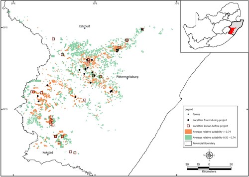
Since the commencement of the study in 2019, 21 additional localities with L. xenodactylus populations have been identified (Figure 1). This brings the total number of known localities to 48, an increase of 77.8%. Twenty of the 21 newly recorded localities were the direct result of using the predicted distribution map to guide field surveys. The mean (± 1 s.d.) predicted relative suitability of habitat for L. xenodactylus at the 21 new locations was 0.59 ± 0.218.

Figure 1. Distribution records for Leptopelis xenodactylus collected prior to (magenta squares) and during (black dots) this study. The areas of average relative suitability for the species (coloured polygons) were obtained from the output of the first distribution model. Inset: the mask area (red; see text) for Leptopelis xenodactylus within the KwaZulu-Natal province (grey area) of South Africa.

Characterisation of the habitat of Leptopelis xenodactylus

The environmental variables that were included in the distribution model and the frequency of occurrence at the localities (n = 48) with records of L. xenodactylus, are presented in Table 1. The dominant vegetation type in which most frogs were located was Temperate Alluvial Wetlands, followed by Mooi River Highland Grassland and Drakensberg Wetlands. The landform type on which the frog species is mostly found is U-shaped valleys. All localities were situated above 1 000 m a.s.l., with most records falling between 1 300 m a.s.l. and 1 900 m a.s.l. and only two records above this range.

Table 1. Variables included in the distribution models according to their frequency of occurrence at locations (n = 48) with Leptopelis xenodactylus.

Variable	Frequency
Vegetation type
Temperate Alluvial Wetlands	22
Mooi River Highland Grassland	10
Drakensberg Wetlands	8
Drakensberg Foothills Moist Grassland	3
Midlands Mistbelt Grassland	2
uKhahlamba Basalt Grassland	2
Eastern Temperate Wetlands	1
Landform type
U-shaped valley	26
Upper slopes, mesas	8
Canyons, deeply incised streams	7
Upland drainages, headwaters	1
Open slopes	1
Mountain tops, high ridges	3
Plains	2
Elevation (m a.s.l.)
1 000–1 300	4
1 301–1 600	17
1 601–1 900	25
1 901–2 000	2
Mean summer monthly potential evaporation (mm)
130–140	5
141–150	12
151–160	31
161–170	1
Variable	Frequency
Average summer mean daily maximum temperature (°C)
21	4
22	8
23	28
24	3
25	4
26	1
Average summer median monthly rainfall (mm)
90–110	8
111–130	30
131–150	9
151–170	1
Average summer mean daily average relative humidity (%)
71–73	4
74–76	19
77–79	20
80–82	5
Plant available water (mm)
30–50	1
51–70	8
71–90	21
91–110	12
111–130	5
131–150	1

Regarding the meso-habitat scale, several common characteristics of the wetlands inhabited by L. xenodactylus were the absence of large areas of open water and the presence of clay-based soil and dense, short emergent vegetation. In wetlands where there was a stream or flowing water, they avoided the flowing areas and were found around the peripheries where the water was almost stagnant. The overriding factors that seemed critical for the presence of these frogs were soil hummocks vegetated with graminoids. Here the adults and eggs were found in burrows and vocalising adult males were found on the soil surface or in vegetation on the hummock.

Distribution Model for inclusion of Leptopelis xenodactylus in spatial planning tools

A regularisation factor of 1.3 and auto features were selected for the model (Supplementary Table S1). The variables most important in determining the predicted distribution of the species, according to their permutation importance, were vegetation type (VEG) and mean summer monthly potential evaporation (PEVAP; Table 2). VEG appeared to have the most useful information when the variables were considered separately (Figure 2). This variable also appeared to have the most information that was not present in the other variables (Figure 2; values shown are averages over the three replicate runs). Figure 3 is the output of the final distribution model for Leptopelis xenodactylus. The mean (± 1 s.d.) average predicted relative suitability of habitat at the localities at which L. xenodactylus has been found, was 0.56 ± 0.280 (n = 48). The two localities with the most suitable habitat (relative suitability (rs) = 0.96) were temperate alluvial wetlands that had relatively low mean summer monthly potential evaporation (140 mm). The two localities with the relatively least suitable habitat (rs = 0.05) were grasslands (two types) that had relatively high mean summer monthly potential evaporation (≥ 148 mm).

Figure 2. Jackknife test of variable importance using training gain (top) and using test gain (middle), and jackknife test of variable importance using area under the receiver operator characteristic curve on test data. See the text for explanation of the acronyms.

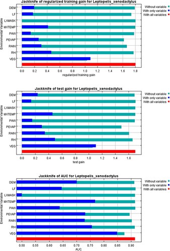
Figure 3. Average relative suitability of areas for Leptopelis xenodactylus within the predicted distribution range.

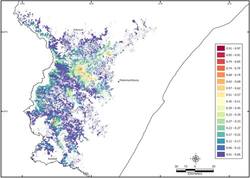
Table 2. Variables included in the MaxEnt environmental niche model for Leptopelis xenodactylus. VEG = vegetation type, RH = average summer relative humidity (%), RAIN = average summer median monthly rainfall (mm), PEVAP = mean summer monthly potential evaporation (mm), LF = landform, PAW = soil plant available water (mm), DEM = elevation (m a.s.l.), MXTEMP = average summer mean daily maximum temperatures (°C). Summer was defined as September to March. See Material and Methods for further explanation of the variables.

Variable	Percent contribution	Permutation importance
VEG	57.3	41.9
RH	14.8	0.3
RAIN	12.7	13.1
PEVAP	6.2	33.0
LF	4.9	6.8
PAW	2.2	0.2
DEM	1.3	4.5
MXTEMP	0.6	0.2

Recalculation of the extent of occurrence (EOO) and area of occupancy (AOO) for Leptopelis xenodactylus and assessing its vulnerability to climate change

The EOO was measured to be 12 006 km² and the AOO was calculated to be 180 km². The results of the climate change vulnerability analysis show that, according to the downscaled GFDL2.1 model and the vulnerability framework, 78% of the localities are considered “Robust” while the remaining 22% are classified as “Vulnerable”. According to the downscaled HadMC2 model and the vulnerability framework, 19.5% of the localities are considered “Robust”, 58.5% are considered “Susceptible” and 22% are considered “Vulnerable” (Table 3).

Table 3. Localities (n = 41) of Leptopelis xenodactylus in relation to the vulnerability framework and the two downscaled climate models (HadCM2 and GFDL2.1; Jewitt et al. 2015a).

	Climate models: HadCM2 (H), GFDL2.1 (G)
	Robust	Susceptible	Constrained	Vulnerable
No. of localities	H: 8 G: 32	H: 24 G: 0	—	H: 9 G: 9
Percentage	H: 19.5 G: 78.0	H: 58.5 G: 0	—	H: 22.0 G: 22.0

Discussion

The initial distribution model for L. xenodactylus was created as a tool to assist with identifying potential localities where the species had yet to be recorded. Due to the initial difficulty in locating these frogs, severe seasonal time constraints, large areas and distances to cover, and limited resources, it was important to narrow the search area as much as possible. This model proved to be a useful tool for finding previously undocumented populations of L. xenodactylus. The model was effective for showing the general area in which the frogs were likely to occur, identifying wetlands apparently suitable for L. xenodactylus and allowing for routes to be chosen that would link the highest number of potential sites for an evening’s trip.

Though the frogs were found in just more than a third of the wetlands that were visited, there are various possible explanations for the species not being recorded in the other wetlands. Absence could not be confirmed if no vocalisations were heard because the frogs may have been present but silent owing to, for example, unsuitable weather conditions such as relatively low temperatures or falling rain (unpublished data). Another reason is that the call does not carry particularly far relative to the calls of some co-occurring frog species, because L. xenodactylus often calls from underground or within thick vegetation (pers. obs.). An observer may need to be near the vocalising frogs to detect them in large wetlands and access to much of these wetlands was sometimes not possible. Their calling season is limited, with most of the vocalising occurring between September and October (unpublished data) and even within this period the males may not vocalise frequently or loudly (pers. obs.), reducing the chances of detecting them. At some localities, the wetlands were degraded to such a degree that they were no longer suitable for the frogs, despite the model’s prediction. Examples of this degradation were wetlands where there was extensive overgrazing by cattle, alien vegetation that had encroached during the dry season and covered a sizeable percentage of the suitable habitat, and canalisation and draining of the wetlands. However, apparent degradation of a wetland did not necessarily indicate that L. xenodactylus was absent, demonstrated by a L. xenodactylus who was recorded vocalising from a remnant wetland identified by the model as potential L. xenodactylus habitat abutting a mature Eucalyptus plantation.

Distribution records show that most historical L. xenodactylus localities were in wetland vegetation types in wide (U-shaped) valleys, with the remainder in grasslands. Resident and sexually mature adults are commonly found in wetlands with slow-moving water suitable for breeding, and forage in adjacent grasslands (pers. obs.). Sexually immature individuals are likely to disperse through grasslands while locating other wetlands (pers. obs.). We found that L. xenodactylus inhabits wetlands that contain hummocks which are mounds of clayey soil covered by grasses surrounded by narrow channels of water. Hummocks are created by earthworm castings over extended periods of time and are mainly concentrated in valley bottoms and floodplain back-swamps in the Drakensberg foothills where accumulations of clay-rich sediments several metres deep are found (Grenfell et al. 2009). From the data available it is unclear if L. xenodactylus is present in wetlands that do not have, and have never had hummocks, or if hummocks are a critical requirement for this species to reproduce. The association of L. xenodactylus with these hummocks could be due to their need to be next to the water for the tadpoles, but at the same time, for adults to be in, or on, soil for the purposes of burrowing, vocalising and egg development. Hummocks may also provide a degree of protection from predators for the adult frogs as well as their eggs, being isolated by the water-filled channels from the land adjacent to the wetland. Further research into these aspects might prove useful for predicting the presence of L. xenodactylus at sites.

Adding the information from the new localities that were located through the output of the first SDM, a second SDM was created. This model can be used for locating more L. xenodactylus populations in future and as a tool in land-use and conservation planning. The model can be used to identify wetlands and adjacent grasslands and grassland linkages between wetlands of relatively high suitability for L. xenodactylus. These areas can be highlighted and significant negative impacts on the overall population of the species potentially avoided by incorporating the model output into land-use decision-making tools. These tools include the spatial development frameworks for local and district municipalities (Spatial Planning and Land Use Management Act) (Republic of South Africa 2013) and the Environmental Screening Tool of the Department of Forestry, Fisheries and the Environment (Republic of South Africa 2021).

In the most recent IUCN red listing exercise for L. xenodactylus (IUCN 2017), the EOO was calculated as 11 000 km² and the AOO as 42 km². The recalculated areas were found to be larger, with the EOO having increased by 9% to 12 006 km² while the AOO increased by 429% to 180 km². A new South African amphibian red listing assessment process started in 2023 and data from this project should be useful for the assessment of L. xenodactylus. A monitoring programme to assist with the early detection of threats to and changes in the populations of L. xenodactylus can be designed and implemented more effectively now that the habitat preferences of the species are known.

One of the major threats facing biodiversity, including amphibians, is climate change (Foden et al. 2013). The results for temperature, rainfall, relative humidity, potential evaporation and plant available water describe a temperate frog species that occurs entirely within a summer rainfall area. The data indicated the presence of both a lower and an upper elevation limit to the distribution of L. xenodactylus. The climate becomes hotter and wetter below the lower elevation limit (Mucina and Rutherford 2006) and at elevations above the upper limit the terrain becomes too steep and precipitous for U-shaped valleys and hummock wetlands to form (Grenfell et al. 2009). The elevational and temperature constraints indicate that the distribution of L. xenodactylus may be influenced by climate change, as observed in other anuran species (Li et al. 2013; Cordier et al. 2020). Downscaling of two climate change models (GFDL2.1 and HadCM2) for the KwaZulu-Natal province of South Africa shows the extremes of the predicted changes, with HadCM2 predicting an average 2.1 °C mean annual temperature increase in KZN, coupled with a mean annual precipitation decrease of 90 mm, while GFDL2.1 predicts a 1.5 °C mean annual temperature increase in KZN with a slight increase in mean annual precipitation of 29 mm (Jewitt et al. 2015a). Both climate change and habitat transformation could be major threats to L. xenodactylus according to the HadCM2 model and the vulnerability framework (affecting up to 80.5% of the geographic range), but not according to the GFDL2.1 model and the vulnerability framework (affecting up to 22% of the geographic range).

The analysis of Botts et al. (2015) suggested that the geographical ranges of most of the amphibian species included in their study that occur mainly in the eastern part of South Africa, have contracted in the past few decades (the study did not include L. xenodactylus). These contractions could not be attributed to climate change, but rather to land cover changes. Leptopelis xenodactylus populations adjacent to transformed areas could be detrimentally impacted by anthropogenic activities (Sutherland et al. 2019). An aspect likely to prove important in the future is the analysis of the land use of the areas surrounding the confirmed L. xenodactylus localities and the distance to the closest human habitations and disturbance (de Baan et al. 2013). Dispersal routes between warmer lower-elevation and cooler higher-elevation hummock wetlands may become transformed through human activities. From this it might be possible to predict which populations are more likely to decline from either anthropomorphic or climate-related change. In time these factors may become a serious challenge to the conservation of L. xenodactylus. If the populations most vulnerable to decline and local extinction can be determined, targeted protection or mitigation measures could be put in place to prevent such outcomes (Dawson et al. 2011).

Should the downscaled HadCM2 model turn out to be a better predictor of future climate change in the distribution of the species, and in the face of further land transformation (Jewitt et al. 2015b), the following conservation measures could be implemented to mitigate the impacts of these factors on the overall population of L. xenodactylus (Jewitt et al. 2015a): (1) increasing the extent of the protected areas in which L. xenodactylus occurs and setting aside new protected areas for the species to maximise their resilience to climate change; (2) avoiding change of land use near wetlands where the species occurs; and (3) maintaining the functioning of the wetland ecosystems and maintaining connectivity between wetlands occupied by the species. Micro-refugia may persist within each domain and these micro-refugia, if protected, could provide safe havens for species (Ashcroft 2010). Better knowledge of the requirements of L. xenodactylus will provide an improved baseline for researchers to enable them to monitor and evaluate trends in overall population size and, as the environment changes, to gain a more informed understanding of the impact of the changes on the L. xenodactylus population. Such understanding will enable mitigation of the threats of climate change and land transformation on L. xenodactylus through appropriate management interventions.

Acknowledgements

We thank Bimall Naidoo for her assistance with producing the map figures, Scotty and Diane Kyle for their assistance with fieldwork, and all the people who contributed locality records for L. xenodactylus for inclusion in Ezemvelo KZN Wildlife’s Biodiversity Database, especially Jeanne Tarrant. We thank the Mohamed bin Zayed Species Conservation Fund and the Oppenheimer Generations Fund for financial support.

Disclosure statement

No potential conflict of interest was reported by the author(s).

References

- Anderson RP. 2012. Harnessing the world’s biodiversity data: promise and peril in ecological niche modeling of species distributions. Ann N Y Acad Sci. 1260:66–80. https://doi.org/10.1111/j.1749-6632.2011.06440.x
- Armstrong AJ. 2001. Conservation status of herpetofauna endemic to KwaZulu-Natal. J Herpetol. 50:79–96.
- Ashcroft MB. 2010. Identifying refugia from climate change. J Biogeogr. 37:1407–1413.
- Botts EA, Erasmus BFN, Alexander GJ. 2015. Observed range dynamics of South African amphibians under conditions of global change. Austral Ecol. 40:309–317. https://doi.org/10.1111/aec.12215
- Cordier JM, Lescano JN, Rios N, Leynaud GC, Nori J. 2020. Climate change threatens micro-endemic amphibians of an important South American high-altitude center of endemism. Amphibia-Reptilia. 41(2):233–243. https://doi.org/10.1163/15685381-20191235
- Dawson TP, Jackson ST, House JI, Prentice IC, Mace GM. 2011. Beyond Predictions: Biodiversity Conservation in a Changing Climate. Science. 332:53–58. https://doi.org/10.1126/science.1200303
- de Baan L, Alkemade R, Koellner T. 2013. Land use impacts on biodiversity in LCA: a global approach. Int J Life Cycle Assess. 18:1216–1230. https://doi.org/10.1007/s11367-012-0412-0
- du Preez LH, Carruthers VC. 2017. Frogs of Southern Africa. Cape Town: Struik Nature
- Eastman JR. 1999. Idrisi 32 guide to GIS and image processing. Worcester, USA: Clark University.
- Elith J, Phillips SJ, Hastie T, Dudik M, En Chee Y, Yates CJ. 2011. A statistical explanation of MaxEnt for ecologists. Divers Distrib. 17:43–57. https://doi.org/10.1111/j.1472-4642.2010.00725.x
- Ezemvelo KZN Wildlife. 2014a. KwaZulu-Natal Average Summer Monthly Means of Daily Maximum Temperature (W31) [Derived from South African Atlas of Climatology and Agrohydrology 2006], Resampled to E KZN W 2008v2 Land Cover Parameters – 2014 Modelling Suite. Unpublished GIS Coverage [AVSUM_MNDMAXTEMP_06_20M_W31_9999.zip]. Pietermaritzburg: Conservation Services, Ezemvelo KZN Wildlife.
- Ezemvelo KZN Wildlife. 2014b. KwaZulu-Natal Average Summer Median Monthly Rainfall (W31) [Derived from South African Atlas of Climatology and Agrohydrology 2006], Resampled to E KZN W 2008v2 Land Cover Parameters – 2014 Modelling Suite. Unpublished GIS Coverage [avsumpotevap_20m_w31_9999.zip]. Pietermaritzburg: Conservation Services, Ezemvelo KZN Wildlife.
- Ezemvelo KZN Wildlife. 2014c. KwaZulu-Natal Average Summer Monthly Means of Daily Average Relative Humidity (W31) [Derived from South African Atlas of Climatology and Agrohydrology 2006], Resampled to E KZN W 2008v2 Land Cover Parameters – 2014 Modelling Suite. Unpublished GIS Coverage [AVSUM_MNDAVRH_06_20M_W31_9999.zip]. Pietermaritzburg: Conservation Services, Ezemvelo KZN Wildlife.
- Ezemvelo KZN Wildlife. 2014d. KwaZulu-Natal Average Summer Potential Evaporation (W31) [Derived from South African Atlas of Climatology and Agrohydrology 2006], Resampled to E KZN W 2008v2 Land Cover Parameters – 2014 Modelling Suite. Unpublished GIS Coverage [avsumpotevap_20m_w31_9999.zip]. Pietermaritzburg: Conservation Services, Ezemvelo KZN Wildlife.
- Ezemvelo KZN Wildlife. 2014e. KwaZulu-Natal Plant available water (W31) [Derived from South African Atlas of Climatology and Agrohydrology 2006], Resampled to E KZN W 2008v2 Land Cover Parameters – 2014 Modelling Suite. Unpublished GIS Coverage [avsumpotevap_20m_w31_9999.zip]. Pietermaritzburg: Conservation Services, Ezemvelo KZN Wildlife.
- Ezemvelo KZN Wildlife. 2015a. KwaZulu-Natal Landform [Derived from modified 30 m SRTM DEM], Resampled to E KZN W 2008v2 Land Cover Parameters – 2014 Modelling Suite. Unpublished GIS Coverage [lf830_20m_w31_9999.zip]. Pietermaritzburg: Conservation Services, Ezemvelo KZN Wildlife.
- Ezemvelo KZN Wildlife. 2015b. KwaZulu-Natal Projected Modified 30 m SRTM DEM (W31) [Derived from DEM sourced from U.S. Geological Survey, Department of the Interior/USGS], Resampled to E KZN W 2008v2 Land Cover Parameters - 2014 Modelling Suite. Unpublished GIS Coverage [SRTM30m_DEM_20m_v2_w31_9999]. Pietermaritzburg: Conservation Services, Ezemvelo KZN Wildlife.
- Ezemvelo KZN Wildlife 2020. KZN Modification Surface – Leptopelis xenodactylus (W31) [Derived from Ezemvelo KZN Wildlife & GEOTERRA Image KZN Land-cover 2017v1], Reclassed & Projected to w31. Unpublished GIS Coverage [KZN_EQV17V1_MOD_LepXen_W31_BF20M_9999.zip]. Pietermaritzburg: Conservation Services, Ezemvelo KZN Wildlife.
- Foden WB, Butchart SHM, Stuart SN, Vié J-C, Akçakaya HR, Angulo A et al. 2013. Identifying the World’s Most Climate Change Vulnerable Species: A Systematic Trait-Based Assessment of all Birds, Amphibians and Corals. PLoS ONE. 8 e65427. https://doi.org/10.1371/journal.pone.0065427
- Grenfell MC, Ellery WN, Grenfell SE. 2009. Valley morphology and sediment cascades within a wetland system in the KwaZulu-Natal Drakensberg Foothills, eastern South Africa. Earth Surf Process Landf. 33:2029–2044. https://doi.org/10.1002/esp.1652
- IUCN Standards and Petitions Committee. 2022. Guidelines for Using the IUCN Red List Categories and Criteria. Version 15.1. Standards and Petitions Committee. https://www.iucnredlist.org/documents/RedListGuidelines.pdf
- IUCN SSC Amphibian Specialist Group, South African Frog Re-assessment Group (SA-FRoG). 2017. Leptopelis xenodactylus The IUCN Red List of Threatened Species 2017:e.T11700A77163657. http://doi.org/10.2305/IUCN.UK.2017-2.RLTS.T11700A77163657.en
- Jewitt D. 2018. Vegetation type conservation targets, status and level of protection in KwaZulu-Natal in 2016. Bothalia. 48:a2294. https://doi.org/10.4102/abc.v48i1.2294
- Jewitt D, Erasmus BFN, Goodman PS, O’Connor TG, Hargrove WW, Maddalena DM. 2015a. Climate-induced change of environmentally defined floristic domains: A conservation based vulnerability framework. Appl Geogr. 63:33–42. https://doi.org/10.1016/j.apgeog.2015.06.004
- Jewitt D, Goodman PS, Erasmus BFN, O’Connor TG, Witkowski ETF. 2015b. Systematic land-cover change in KwaZulu-Natal, South Africa: Implications for biodiversity. SA J Sci. 111:2015–0019. https://doi.org/10.17159/sajs.2015/20150019
- Junior PDM, Nobrega CC. 2018. Evaluating collinearity effects on species distribution models: An approach based on virtual species simulation. PLoS ONE. 13:e0202403. https://doi.org/10.1371/journal.pone.0202403
- Li Y, Cohen JM, Rohr JR. 2013. Review and synthesis of the effects of climate change on amphibians. Intergr Zool. 8:145–161. https://doi.org/10.1111/1749-4877.12001
- Mawdsley JR, O’Malley R, Ojima DS. 2009. A Review of Climate-Change Adaptation Strategies for Wildlife Management and Biodiversity Conservation. Conserv Biol. 23:1080-1089. https://doi.org/10.1111/j.1523-1739.2009.01264.x
- Mayani-Paras F, Botello F, Castaneda S, Sanches-Cordero V. 2019. Impact of Habitat Loss and Mining on the Distribution of Endemic Species of Amphibians and Reptiles in Mexico. Diversity 11:210. https://doi.org/10.3390/d11110210
- Merow C, Smith MJ, Silander JA. 2013. A practical guide to MaxEnt for modeling species’ distributions: what it does, and why inputs and settings matter. Ecography. 36:1058–1069. https://doi.org/10.1111/j.1600-0587.2013.07872.x
- Minter LR, Burger M, Harrison J, Braack H, Bishop PJ, Kloepfer D. 2004. Atlas and Red Data Book of the Frogs of South Africa, Lesotho and Swaziland. Washington DC: Smithsonian Institution.
- Mittermeier RA, Gil PR, Hoffman M, Pilgrim J, Brooks T, Mittermeier CG et al. 2005. Hotspots Revisited: Earth’s biologically richest and most endangered ecoregions. Chicago: University of Chicago Press.
- Morales NS, Fernandez IC, Baca-Gonzalez V. 2017. MaxEnt’s parameter configuration and small samples: are we paying attention to recommendations? A systematic review. PeerJ. 5:e3093. https://doi.org/10.7717/peerj.3093
- Mucina L, Rutherford MC. 2006. The Vegetation of South Africa, Lesotho and Swaziland. Pretoria, South Africa: South African National Biodiversity Institute.
- Ortega-Andrade HM, Rodes Blanco M, Cisneros-Heredia DF, Guerra Arévalo N, López De Vargas-Machuca KG, Sánchez-Nivicela JC et al. 2021. Red List assessment of amphibian species of Ecuador: A multidimensional approach for their conservation. PLoS ONE. 16:e0251027. https://doi.org/10.1371/journal.pone.0251027
- Peterson AT. 2001. Predicting species’ geographic distributions based on ecological niche modeling. Condor. 103:599–605. https://doi.org/10.1093/condor/103.3.599
- Peterson AT, Soberón J. 2012. Species distribution modeling and ecological niche modeling: Getting the concepts right. Nat Conserv. 10:1–6. https://doi.org/10.4322/natcon.2012.019
- Peterson AT, Soberón J, Pearson RG, Anderson RP, Martínez-Meyer E, Nakamura M, Araújo MB. 2011. Ecological niches and geographic distributions. Princeton: Princeton University Press.
- Phillips SJ, Anderson RP, Schapire RE. 2006. Maximum entropy modelling of species geographic distributions. Ecol Model. 190:231–259. https://doi.org/10.1016/j.ecolmodel.2005.03.026
- Phillips SJ, Dudik M. 2008. Modeling of species distributions with MaxEnt: New extensions and a comprehensive evaluation. Ecography. 31:161–175. https://doi.org/10.1111/j.0906-7590.2008.5203.x
- Republic of South Africa. 2013. Spatial Planning and Land Use Management Act, 5 August, Government Gazette Vol. 578, No. 36730.
- Republic of South Africa. 2021. Environmental Screening Tool of the Department of Forestry, Fisheries and the Environment. https://screening.environment.gov.za/screeningtool/#/pages/welcome
- Schulze RE. 2006. South African Atlas of Climatology and Agrohydrology. Pretoria, South Africa: Pretoria Water Research Commission.
- Scott-Shaw CR, Escott BJ (Editors). 2011. KwaZulu-Natal Provincial Pre-Transformation Vegetation Type Map – 2011 v2.4, Rasterized to E KZN W 2008v2 Land Cover Parameters - 2014 Modelling Suite. Unpublished GIS Coverage [kznveg05v2_4_11_inhouse_w31_03022020_20m_9999.zip]. Pietermaritzburg: Biodiversity Conservation Planning Division, Ezemvelo KZN Wildlife.
- Simoes M, Romero-Álvares D, Nunez-Penichet C, Jiménez LJ, Cobos ME. 2020. General theory and good practices in ecological niche modeling: A basic guide. Biodivers Inform. 15:67–68. Haste
- Sutherland WJ, Dicks LV, Ockendon N, Petrovan SO, Smith RK. 2019. What Works in Conservation. Cambridge: Open Book Publishers.
- Tarrant J, Armstrong AJ. 2013. Using predictive modelling to guide the conservation of a critically endangered coastal wetland amphibian. J Nat Conserv. 21:369–381. https://doi.org/10.1016/j.jnc.2013.03.006
- Warren DL. 2012. In defense of ‘niche modeling’. Trends Ecol Evol. 27:497–500. https://doi.org/10.1016/j.tree.2012.03.010