Field-independent carbon mapping and quantification in forest plantation through remote sensing

ABSTRACT

Quantifying the carbon-stocking contribution of forest plantations is a crucial but challenging and expensive process, usually performed through field analysis. For this reason, plantations’ carbon storage is often calculated and reported using generic and inaccurate functions relying exclusively on tree species and plantation age. This study introduces a new field-independent (FI) method for forest plantations’ carbon quantification and mapping through automatic analysis of Sentinel-2 data. The study area is a Guatemalan forest plantation of 20 hectares, for which we constructed a reference dataset measuring in the field the diameter and the height of all trees within 20 randomly selected plots (10-meter radius). The CO2 equivalent absorbed by the plantation was first estimated using ground data and a design-based (DB) approach. Then, to obtain CO2 equivalent estimates but also maps, we used both ground and Sentinel-2 data to compare a standard model-assisted (MA) approach relying on Random Forests with the FI approach. Our results demonstrate that the FI method provides carbon stock statistics comparable to those obtained using DB and MA methods and more accurate maps. Accordingly, the RMSE obtained using the FI method was 34% while that obtained by the MA method – exploiting random forest algorithm – was greater (RMSE = 39%). The 95% confidence interval estimates of the CO2 stored in the plantation were 100 ± 18 MgC ha−1 and 102 ± 8 MgC ha−1, for DB and MA respectively. Using the FI method, the CO2 ranged between 89 and 117 Mg C ha−1, all values within the DB confidence interval. In addition, the FI map was surprisingly consistent with the MA-derived map, making our approach a valid alternative for monitoring plantation status and carbon storage when ground data are not available.

KEYWORDS:

• Sentinel-2
• forest
• Google Earth Engine
• machine learning
• estimates
• confidence intervals

Introduction

Mitigating the effects of climate change is a critical societal objective now and in the forthcoming decades. Approximately 10% of the world’s annual total carbon emissions are due to deforestation and forest degradation in tropical countries (Csillik et al., 2019). In the interim, carbon dioxide can be removed from the atmosphere and can help limit global warming through sustainable forest management and replanting operations (IPCC, 2018). Thus, national and international initiatives such as REDD+ (Reducing Emissions from Deforestation and Forest Degradation) are dedicated to addressing those issues. Specifically, to counteract global warming, each country’s carbon emissions from deforestation and forest degradation must be estimated and monitored over time (Csillik et al., 2019). At such expansive geographic scales, an accurate, economical, and high-resolution method of tracking changes in aboveground carbon inventories is required.

Preventing serious climate change requires removing carbon dioxide from the atmosphere as well as making significant cutbacks to emissions. Forests are a vital element of the global carbon cycle and are proven to be the major terrestrial sink for carbon (Yang et al., 2022). As a result, the G20 summit (Rome) proposal from November 2021 to plant 1 billion trees by 2030 to address the climate issue has been approved, as tree restoration and emissions reduction have been included among the most successful measures for mitigating climate change. Accordingly, the restoration of tropical agricultural landscapes, due to the quantity of area available and the growth rate of the trees, has some of the highest potential to counteract climate change (Bastin et al., 2019). However, quantifying the contribution of carbon stocking leads to new forest plantations is an arduous process that is typically characterized as being expensive and time-consuming.

Due to the high degree of knowledge and reliable scientific procedures required for carbon stock assessment, many reforestation programs find it challenging to scale up since it is difficult to provide reliable evidence of good outcomes. This is a major issue in light of the recent and substantial financing commitments made to forest restoration efforts (Cavanagh et al., 2021; Fairhead et al., 2012; Tucker et al., 2023). Seriously, many plantations, afforestation, or REDD+ projects experienced failure due to a wrong estimation of the carbon sequestration capacity (Lederer, 2011; Li et al., 2022). Since it is well known that the certification process for carbon credits is tough and complex, reliable estimating methods founded on sound scientific principles must be the starting point.

Traditionally, forest carbon stocks have been estimated using field plot networks by correlating tree structural characteristics (diameter, height, and wood density) to aboveground carbon density (ACD) using allometric equations (Csillik et al., 2019). The aboveground biomass (AGB) of trees – and thus the amount of carbon stored – is indeed known to be very correlated with different morphological features (Harris et al., 2021; Schepaschenko et al., 2021; Vangi et al., 2023; Xu et al., 2021). For example, the tree diameter – by convention measured at breast height or 1.3 m (diameter at breast height, DBH) – is highly correlated with the total AGB (Brown, 1997; Brown et al., 1989; Chave et al., 2005; Stass, 2011). Likewise, belowground biomass (BGB) is often calculated as a function of AGB. AGB species-specific equations typically increase estimation accuracy (Fayolle et al., 2013; Rutishauser et al., 2013). On the other hand, relationships between DBH and tree height have been found to vary across environmental conditions, reducing the importance of species type in determining the accuracy of the equation (Fayolle et al., 2013; Feldpausch et al., 2012). In addition, Chave et al (Chave et al., 2005). showed that a single equation including tree diameter, wood-specific density, and total tree height already provides a precise estimate of AGB and that including site, successional status, the continent or forest type only slightly improves the precision of the estimate (Pati et al., 2022). Along with the previously mentioned studies, current scientific research demonstrates how the AGB and carbon stock of individual trees can be estimated by measuring their heights and diameters.

Unfortunately, forest information systems that solely rely on ground data present several drawbacks (Katila et al., 2015; Latifi et al., 2015; Tomppo et al., 2010). First, gathering ground data and conducting fieldwork is both expensive and time-consuming. Second, the lengthy re-measurement intervals hinder their ability to capture recent changes. Third, while the acquired data may be combined to create statistics, they are unable to create continuous and geographically detailed information on their own, which may be more beneficial from a management standpoint. Fourth, combining data and performing statistically valid comparisons is difficult since data are collected through various methodologies and criteria. Fifth, the expensive data collected on the ground is rarely available or open access. To overcome those issues and to increase the precision and frequency of forest monitoring, several studies have suggested methodologies involving the combination of field and remote sensing data.

Recent developments in machine learning (ML) (D'Amico et al., 2021) and the expanding availability of satellite images have created new and cost-effective ways to monitor reforestation activities (Bozzini et al., 2023; Cavalli et al., 2022, 2023; Francini et al., 2023). However, relying entirely on remote sensing data without calibration through ground field data, especially at the scale of smallholder farmers, could lead to insufficient evaluation and large inaccuracies. Indeed, to calibrate ML models for the interpretation of remote sensing data and to gather consistent, and reliable statistics, field information is crucial (Griscom et al., 2017). For example, the carbon content within trees varies significantly between forest types and other vegetation cover types (Asner et al., 2013b) making it necessary to have ground data for an accurate interpretation of satellite imagery. Additionally, field information is crucial for successfully managing smallholder carbon projects, such as obtaining seedling counts on parcels, tracking forest management practices, and managing farmer visits (Griscom et al., 2017).

However, coupling remote sensing with field data also presents some limitations, mainly because ground measurements and forest inventories have been historically conducted to provide estimates of variables of interest and not data useful to be combined with remote sensing and constructing models. In this sense, areas measured on the ground (plots) are usually too small to be combined with remote sensing medium-resolution imagery, such as those acquired by Sentinel-2 and Landsat satellite missions. This limitation is amplified by ground positioning errors, as decreasing the precision of the coordinates attributed to the plots further complicates coupling ground and remote sensing data. In summary, several methods for monitoring the carbon storage of tree plantations exist and both main groups of methodologies to do so – those relying exclusively on field data and those coupling field and remote sensing data – present several limitations.

This research aims to present a method for providing maps and statistics of tree plantations’ carbon storage using exclusively remote sensing data, thus without requiring field analysis (hereinafter referred to as the Field-independent approach, FI). Accordingly, a model that allows quantifying and defining patterns of carbon distribution across the forest plantation requiring just general information on the plantation without any field survey was constructed. To this end, we tested different approaches in which plantation knowledge was increasingly detailed (from just species and plantation age to the average diameter and height of trees within the plantation) (section 3.3.1). For comparison purposes, we also integrated Sentinel-2 open-access imagery and ground data through a model-assisted (MA) approach, and we conducted a statistical analysis of the differences between the carbon stock maps’ accuracy and statistics obtained using (section 3.2) and without using (section 3.3) ground data. Finally, as a benchmark, the plantations’ carbon storage was estimated using exclusively ground data and a design-based (DB) approach (section 3.1).

Materials

Study area

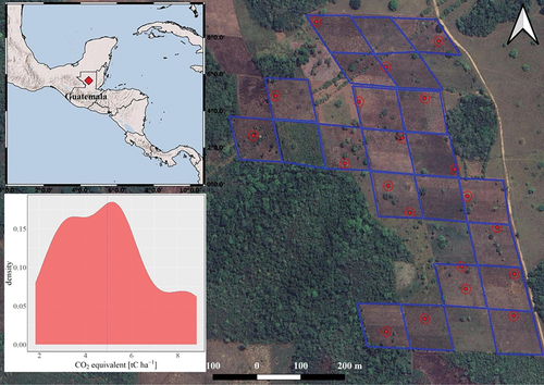
The study area consists of a tree plantation of 20.31 ha located in the community of Montecarmelo in the commune of La Libertad in the Petén department, Guatemala (16° 50’59.57 “N; 90° 2’39.24” W) (Figure 1). The study area includes 1111 trees per hectare, for a total of about 22,500 trees. Each tree is given nine square meters of space. Half of the trees in the study area are cedar (Cedrela odorata L.) and the remaining half is mahogany (Swietenia macrophylla King.), both species of great cultural and economic importance (UNEP-WCMC, 2009). Trees were planted in the open field at 6 months of age, resulting in a 21-month-old plantation at the time of the field measurements (June 2022). The two species are planted alternately with each other across the study area.

Figure 1. The study area (blue) and sample plots (red). Bottom-left, the density distribution of the CO₂ equivalent in the 20 plots measured on the ground.

Ground data

For training and validating different models and estimating the amount of carbon stored in the study area, we constructed a reference sample by randomly selecting 20 plots (10-m radius or 314 square meters) within the study area (Figure 1). For each plot, the species, the height, and the DBH of each tree were measured allowing the CO₂ equivalent estimation. In total, 730 trees were measured on the ground. Half were cedar and half were mahogany. The surveys were carried out in June 2022 during the leaf-on season, when each tree was 21 months old.

CO₂ calculation

According to Chave et al. (2005), the AGB for cedar and mahogany was calculated as:

(1) $\mathrm{AGB}=0.0673{\left(\mathrm{WD}{\mathrm{D}}^2\mathrm{H}\right)}^{0.976}$(1)

Where AGB is the above-ground biomass, WD is the species-specific wood density, D is the tree DBH, and H is the tree height. For each tree in the plots, tree DBH and tree height were measured during the ground survey (section 2.2). The wood densities for the two species are 0.4 for cedar and 0.5 for mahogany (Zanne et al., 2010). Then, the function of Mokany et al (Mokay et al., 2006), allowed us to calculate the belowground biomass for each tree:

(2) $\mathrm{BGB}=0.489\mathrm{AG}{\mathrm{B}}^{0.89}$(2)

where BGB is the below-ground biomass. The constant 0.489 is the root shot ratio commonly used for tree species.

BGB is a critical component of stored carbon in forests. However, as with AGB, it is challenging to measure BGB directly, given the laboriousness of the direct measurement procedure (extracting, drying, and weighing whole tree root structures). The alternative of developing forest-type or country-specific allometric equations for root biomass is also resource-intensive. While it is acceptable for BGB to be calculated indirectly. For this purpose, already available equations that reliably predict root biomass based on above-ground are used. Then, the total biomass (Bt) was the sum of above and below-ground biomass:

(3) $\mathrm{Bt}=\mathrm{AGB}+\mathrm{BGB}$(3)

The total carbon content was calculated by applying the default carbon fraction factor of 0.5 provided by the IPCC (Penman et al., 2006):

(4) $\mathrm{Ct}=\mathrm{Bt}/2$(4)

Where Ct is the total carbon content. Finally, the equivalent CO₂ content was calculated using a conversion factor derived from the CO₂ molecular weight:

(5) $\mathrm{C}{\mathrm{O}}_{2\mathrm{eq}}=\mathrm{Ct}\left(3.6667\right)$(5)

Sentinel-2 data

Sentinel-2 mission has a wide swath (290 km) with a spatial resolution of 10 to 60-m, depending on spectral bandpass, and a revisit frequency of 2–5 days depending on the latitude (Baetens et al., 2019). The Sentinel-2 Multispectral Instrument (MSI) includes three visible (blue, green, red) and NIR bands at the 10-m resolution and Red edge (redE1, redE2, redE3, redE4), and SWIR (swir1, swir2) bands at the 20-m resolution, which were used in this study (Francini et al., 2022).

An up-to-date Sentinel-2 image archive can be found in the Google Earth Engine (Gorelick et al., 2017), from which we selected all Sentinel-2 images acquired over the study area and during the dry season. More specifically, all images with a cloud coverage of less than 70% and acquired between 15 December 2021 and 15 March 2022 were selected. Then, a cloud-free composite was produced by the state-of-the-art medoid methodology (Kennedy et al., 2018). The medoid processing aims to populate the final image composite with the pixels with surface reflectance values as similar as possible to the median calculated considering the whole image collection. In brief, medoid compares each band’s pixel surface reflectance values to the median bands’ spectral values of that pixel in all selected images. Then, the bands’ spectral values from the pixel closest to that median value (using Euclidean spectral distance) were chosen. As a result of this step, we obtained a cloud-free medoid composite for our area of interest, from which we calculated seven spectral indices: (i) Normalized Difference Vegetation Index (NDVI), (ii) Normalized Burned Ratio (NBR), (iii) Enhanced Vegetation Index (EVI), and (iv) Tasselled Cap Brightness, Wetness, Greenness, and Angle (TCB, TCW, TCG, TCA). The NDVI index (Eq. 6) has been among the most popular indices used to quickly delineate vegetation and vegetative stress. Hence, it shows dense vegetation with high positive values, soil with low positive values, and water with negative values (Alcaras et al., 2022; Huang et al., 2021).

(6) $\mathrm{NDVI}=\left(\mathrm{NIR}-\mathrm{RED}\right)/\left(\mathrm{NIR}+\mathrm{RED}\right)$(6)

Where NIR is the light reflected in the near-infrared spectrum, and RED is the light reflected in the red range of the spectrum.

Similar in the equation to NDVI, the NBR (Eq. 7) is an index designated to highlight burnt areas and fire severity (Key & Benson, 2006). NBR has been used to examine post-fire vegetation recovery (Bright et al., 2019), wildfire severity (Tran et al., 2018) and harvesting (Kennedy et al., 2010), and drought events (Francini et al., 2021; M. C. Hansen et al., 2013; Kennedy et al., 2010). The equation of NBR combines the use of NIR and the ShortWaved InfraRed wavelengths.

(7) $\mathrm{NBR}=\left(\mathrm{NIR}-\mathrm{SWIR}\right)/\left(\mathrm{NIR}+\mathrm{SWIR}\right)$(7)

The EVI (Eq. 8) has been considered a modified NDVI (Matsushita et al., 2007) given its improved sensitivity to high biomass regions and improved vegetation monitoring capability. Indeed, it does not saturate as rapidly as NDVI in dense vegetation and it has been shown to be highly correlated with photosynthesis activity, plant transpiration, and vegetation biomass (X. Jiang et al., 2008; Sims et al., 2006). EVI was calculated as:

(8) $\mathrm{EVI}=\mathrm{G}\left(\mathrm{NIR}-\mathrm{RED}\right)/\mathrm{NIR}+\left(\mathrm{C}1\mathrm{RED}+\mathrm{C}2\mathrm{BLUE}\right)+\mathrm{L}$(8)

where BLUE, RED, and NIR represent the reflectance at the respective wavelengths, L is a soil adjustment factor, and C1 and C2 are coefficients used to correct aerosol scattering in the red band by the use of the blue band, and G is the gain factor, usually set at 2.5 (Shammi & Meng, 2021; Vijith & Dodge-Wan, 2019).

Lastly, the TC (Crist & Cicone, 1984) with its components, i.e. brightness (TCB), greenness (TCG), and wetness (TCW), represent an inherent property of terrestrial reflectance. TCB is a weighted sum of all the bands and accounts for the most variability in the image. It is typically associated with bare or partially covered soil, natural and man-made features, and variations in topography. TCG is a measure of the contrast between the NIR band and the visible bands due to the scattering of infrared radiation resulting from the cellular structure of green vegetation and the absorption of visible radiation by plant pigments. The third component, TCW, is associated with soil moisture, water, and other moist features (Shi & Xu, 2019; Zoka et al., 2018).

The Tasseled Cap Angle (TCA), defined as the angle formed by TCG and TCB in the vegetation plane (Eq. 9), condenses in a single value the information of the relation TCG/TCB and represents the proportion of vegetation to non-vegetation essentially.

(9) $\mathrm{TCA}=\mathit{arctan}\left(\mathrm{TCG}/\mathrm{TCB}\right)$(9)

The three components of TC have been used to develop soil indices (Qiu et al., 2017), to monitor deforestation (Schultz et al., 2016), and for vegetation classification (Macintyre et al., 2020). Studies have shown that dense cover classes of coniferous forests exhibit higher TCG and lower TCB values than open stands or clearcuts (Cohen et al., 1995, 1998). Accordingly, dense forest stands show higher TCA values than more open stands or bare soil. TCA was also used to monitor desertification (Liu et al., 2018), and characterize forest structure (Cohen et al., 2002; A. J. Hansen et al., 2001), successional state (Helmer et al., 2000), changes (Gómez et al., 2011), and condition (Healey et al., 2006; Wulder et al., 2006).

Carbon-monitoring methods

First, the CO₂ equivalent absorbed by the plantation was estimated using exclusively ground data and a DB approach (section 3.1). Second, we used both ground data and Sentinel-2 data within a MA approach (section 3.2). Third, the CO₂ equivalent absorbed by the plantation was estimated using a FI approach, thus using just Sentinel-2 data and ignoring data collected on the ground (section 3.3).

Design based

The mean CO₂ equivalent absorbed by the plantation was inferred using the Horwitz and Thompson (HT) design-based estimators (Horwitz & Thompson, 1952). The HT estimators allow an unbiased estimation of the sampling variance. The HT estimator for the mean is calculated as follows:_

(10) ${\hat{\mu }}_{\mathit{HT}}=\mathit{y}$(10)

where ${\hat{\mu }}_{\mathit{HT}}$ is the sample mean, with a standard error (SE) in the following form:

(11) $\mathit{SE}\left({\hat{\mu }}_{\mathit{HT}}\right)=\sqrt{\frac{{\sigma }^2}{\mathit{n}}}$(11)

where σ² and n are the sample variance and size, respectively.

The HT estimator for the total is:_

(12) ${\hat{\tau }}_{\mathit{HT}}=\mathit{N}\underset{}{y}$(12)

Where N is the population size or the number of pixels in the study area. The SE estimator of the total is:

(13) $\mathit{SE}\left(\mathit{\hspace{0.17em}}{\hat{\tau }}_{\mathit{HT}}\right)\mathit{\hspace{0.17em}}=\sqrt{N^2\frac{{\sigma }^2}{\mathit{n}}}$(13)

Model-assisted

The MA framework (McRoberts et al., 2016) represents the benchmark for RS-based estimates of forest variables (Chirici, Giannetti, Mazza, et al., 2020; D’Amico, Francini, et al., 2021; Francini et al., 2020, 2021; Vangi et al., 2022, 2023) such as CO₂ equivalent absorbed. In the MA estimation, a model exploiting RS data is used as auxiliary information to enhance the inference, while the estimation variance is based on the probability sample (Särndal et al., 1992). The model exploited in this study was random forests (RF), a well-established machine learning algorithm based on an ensemble of decision trees, known for being able to deal with overfitting and predictors autocorrelation (Breiman, 2001). RF is also known to be a good choice when there is a little amount of training data available (Dai et al., 2021; Emick et al., 2023; Francini et al., 2023). In this study, we exploited the randomForest R package (Liaw & Wiener, 2002) and we set two as the number of features considered by each tree when splitting a node and 500 as the number of trees in the forest. Such hyperparameter calibration follows the procedure shown by Vaglio Laurin et al. (2021)and Hawryło et al. (2020) and implies the implementation of the leave-one-out cross-validation procedure (LOOCV).

LOO was also exploited to evaluate the performance of the RF model. One at a time, each of the 20 reference units available was predicted using the remaining reference set units (McRoberts et al., 2015). The number of plots in the reference dataset and thus the number of iterations in the LOO procedure was 20. The final model performance was assessed in terms of percentage root means squared error (RMSE%) and r².

RMSE% was calculated as follows:

(14) $\mathit{RMSE}\%=\frac{\sqrt{\frac{{\sum }_{i=1}^n{\left(y_i-\hat{y}\right)}^2}{\mathit{n}}}}{\bar{y}}\ast 100$(14)

where y_i is the predicted carbon stock in the i^th plot, $\hat{y}$ is the observed carbon stock in the i^th plot, n is the number of plots and $\bar{y}$ is the mean observed carbon stock.

Finally, we assessed the importance of the predictor variables in terms of the percentage increase in Mean Square Error (MSE%) as produced by the RF model. MSE% is a fundamental outcome of RF, and by expressing how much accuracy the model gains by exploiting each variable, it shows how important each variable is for the classification task. The larger the MSE% gain, the more important the variable is for the successful classification (Liaw & Wiener, 2002).

The MA estimator for the mean corresponds to the HT estimator, corrected by a term that takes into account the systematic error of the model, based on the mean residuals of the sample plots:

(15) ${\hat{\mu }}_{\mathit{ma}}=\frac{1}{N}{\sum }_{i=1}^N{\hat{y}}_{\mathit{i}}-\frac{1}{n}{\sum }_{j=1}^n\left({\hat{y}}_{\mathit{j}}-y_j\right)$(15)

The SE for the MA estimator is expressed by:

(16) $\mathit{SE}\left({\hat{\mu }}_{\mathit{ma}}\right)=\sqrt{\frac{1}{\mathit{n}\left(\mathit{n}-1\right)}{\sum }_{j=1}^n{\left(e_j-\underset{-}{e}\right)}^2}$(16)

As a result of this step, we obtained both the estimate of the stored CO₂ by the plantation and the respective map over the study area.

Field independent

Here, we describe a new field-independent method (FI) for the estimation of the CO₂ equivalent absorbed by tree plantations. FI does not require field measurements and indeed did not exploit the 20 plots in the reference dataset. In addition to Sentinel-2 data, FI requires three input parameters: minimum, mean, and maximum CO₂ equivalent per hectare in the forest plantation. This information can be obtained through different approaches without requiring ground data and can provide a different level of precision depending on the availability of tree plantation information (section 3.3.1).

First, we conducted a literature review of the Sentinel-2 predictors (bands and indices, section 2.3) to discriminate them into positive or negatively correlated with CO₂. Second, for each band, we subtracted the mean values of the band from each band’s values (centering) and we divided each new value by the sum between the band range differences and the average C obtained with the allometric equations (scaling). Third, we rescaled the new values to the C minimum and maximum obtained from the allometric equations (rescaling). For predictors positively correlated (NDVI, EVI, and NBR), the 5th and 95th percentile of the predictors were mapped with the minimum and maximum value of CO₂ equivalent absorbed. For predictors negatively correlated (the raw Sentinel-2 bands and the TC indices) we did the opposite: the 95th and 5th percentile of the predictors were mapped with the minimum and maximum. We choose to use the 5th and 95th percentile instead of minimum and maximum values in the predictors to avoid mapping the values derived by the user input with probable outliers or rare reflectance occurrences that would bias the predictions. Indeed, the minimum value in a reflectance band or a vegetation index often corresponds to non-vegetated pixels or vegetation under particular conditions (such as after a disturbance). In contrast, the maximum value may represent an isolated condition in the image or a saturation spot. We remove outliers based on the Interquartile Range (IQR), i.e. the difference between the 3^rd and the 1^st quartiles (Q3 and Q1, respectively). In particular, values greater than Q3 plus 1.5 times the IQR or smaller then Q3 less 1.5 times the IQR were considered outliers. Fourth and last, the CO₂ map is obtained by averaging the values of all rescaled predictors.

While to validate the RF model we used a LOO procedure, here the ground data was not used to construct the model, and thus all the 20 plots in the reference dataset can be used to assess the performance of the FI model in terms of RMSE% and r².

Users simulation

As the FI method also requires general plantation information, in this study, we hypothesized four users with different levels of knowledge about the plantation and thus with different abilities to provide detailed information about the same, from which to calculate FI input parameters, i.e. minimum, mean, and maximum CO₂ equivalent per hectare. To simulate these different levels of operator knowledge about plantations, we tested various strategies by progressively increasing the information available (Table 1). In case a, only age, species, and planting density are known, as well as site characteristics. Because of its basic nature, this background information is generally available or easily and quickly accessible. In case b, also the average diameter of the plantation is known, while in case c, the average height is also available. Finally, in case d, information on the range of the possible CO₂ equivalent values in the plantation is available. This last case can be considered the benchmark for other FI cases, as the exact information needed by the FI model is known. Considering the homogeneity in tree growth that generally occurs in arboriculture plantings, even this information may be available from experienced users who are diffusely familiar with the plantation and its measure ranges. The different data considered available for the four different users are reported in Table 1.

Table 1. Parameters used in the different strategies by progressively increasing the level of plantation knowledge. The FI model requires the information available for user d. The information available for users a, b, and c are used to obtain the information available for user d as detailed below.

User	Plantation available information
a	Tree Species	Planting Density	Age	Site index
b	Tree Species	Planting Density	Average DBH
c	Tree Species	Planting Density	Average DBH	Average Height
d	Min, mean, and max CO2 equivalent

For cases a and b, we calculated AGB using an optimization from Chave et al (2014, 2017). of the AGB equation:

(17) $\mathit{AGB}=e^{\left(-2.024-0.896\mathit{E}+0.92\mathit{ln}\left(\mathit{WD}\right)+2.795ln\left(D\right)-0.0461ln\left(D^2\right)\right)}$(17)

where the AGB is the above-ground biomass, E is a measure of environmental stress (Chave et al., 2014), WD is the species-specific wood density, and D the DBH. For case a, the latter can be estimated with the formula developed by the Instituto Nacional de Bosques (INAB) of Guatemala:

(18) $\mathit{DBH}=e^{\left(\alpha -\frac{\beta }{T}+\mathit{\gamma }\times \mathit{S}-\mathit{\delta }\times \mathit{N}\right)}$(18)

where T is the tree age in year, N is the tree density (N ha⁻¹) and S is the site index, derived from the dominant height of the analyzed plantations of the INAB database in the permanent parcels. In this study, despite the good condition of the plantation, an average value of S was always used to take a conservative approach, 14.7 per Switenia macrophylla and 12.4 per Cedrela odorata respectively. Parameters $\mathit{\alpha }$, $\mathit{\beta },\mathit{\gamma and\delta }$, for Switenia macrophylla and Cedrela odorata, are presented in Table 2.

Table 2. Parameters for estimating the diameter of switenia macrophylla and cedrela odorata (INB, 2019a, 2019b).

Tree species	α	β	γ	δ
Switenia macrophylla	1.724193	2.74867	0.0838	0.000075
Cedrela odorata	2.186717	2.865757	0.079924	0.000238

In case b, equation 17(17) $\mathit{AGB}=e^{\left(-2.024-0.896\mathit{E}+0.92\mathit{ln}\left(\mathit{WD}\right)+2.795ln\left(D\right)-0.0461ln\left(D^2\right)\right)}$(17) was used with the DBH already available from the knowledge of the user. In case c, on the other hand, having tree diameter, tree height, and tree species, the generalized allometric model, equation 1(1) $\mathrm{AGB}=0.0673{\left(\mathrm{WD}{\mathrm{D}}^2\mathrm{H}\right)}^{0.976}$(1) (par 2.3) from Chave et al. (2014) can be used. The values used to implement the different strategies are shown in Table 3.

Table 3. Data used for the different strategies by progressively increasing the level of plantation knowledge and thus of information available to calculate the parameters required by the FI approach: min, mean, and max CO₂ equivalent in the plantation. User d is not reported as it is the benchmark in which min, mean, and max CO₂ equivalent in the plantation are known.

User	Age	Tree Species	Density (N h^−1)	Site index	DBH (cm)	H (m)
a	21 months	S. macrophylla C. odorata	1111	14.7 12.4
b		S. macrophylla C. odorata	1111		4.34 4.10
c		S. macrophylla C. odorata	1111		4.34 4.10	3.81 3.69

Results

The results for each method described above are reported in Table 4, where the estimates of the total CO₂ equivalent absorbed by the plantation are provided, along with the RMSE% and r².

Table 4. Comparison of the results achieved using the DB, MA, and FI carbon mapping and estimation methods. For the DB estimation methods RMSE% and r² are not available as it provides just estimates and not maps. For the FIs methods, confidence intervals are not available as they are based just on remote sensing data, and reference data is not used.

Estimation method	CO2 equivalent (MgC)	RMSE%	r^2
DB	100.5 ± 18.2*	–	–
MA	102.0 ± 8.2*	38.7	0.1
FIa	89.3	39.6	0.3
FIb	117.4	41.9
FIc	102.3	37.3
FId	108.5	34.1

*95% confidence interval estimates.

The CO₂ equivalent absorbed by the plantation is comparable among estimation methods as well as the RMSE%. FIa and FIb lead to the minimum and maximum CO₂ values, respectively, while, notably, the FIc method obtained the same mean value as the MA method but with a lower RMSE% and a much higher r². FId can be considered the benchmark for the FI estimation method, as it represents the case in which FI parameters or minimum, mean, and maximum CO₂ equivalent are known. Accordingly, FId reached the lowest RMSE% and CO₂ equivalent statistics within the confidence interval resulting from the well-established DB and MA methods.

The r² is 0.31 for each FI method, as the final CO₂ maps’ pattern is the same while the range of values changes (Figure 2). Indeed, the maps differ only in the magnitude of absorbed CO₂ values, maintaining identical patterns, due to using the same vegetation indices for all FI methods.

Figure 2. Top, map of CO₂ equivalent obtained with FI method with different CO₂ equivalent ranges (MgC ha⁻¹) depending on the FI case. Bottom, map of CO₂ equivalent obtained with the MA method. Empty pixels correspond to outliers and were masked out.

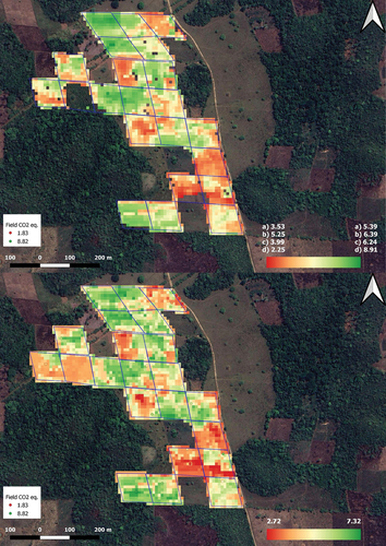
While the FI method we introduced is simple and does not require reference data, the r² and the RMSE% we obtained indicate at least comparable performance to the MA method (Table 4). Although a simple method, our results suggest that FI methods can be a valid alternative to the MA one in the case of tree plantations and when ground data is not available.

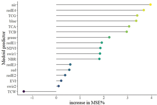
Finally, in Figure 3 we report the importance of the different medoid predictors assessed through the RF model. The Sentine-2 nir band had the greatest impact in increasing the performance of the model while the Tasselled Cap Wettness index (TCW) was useless and even decreased the accuracy of the model.

Figure 3. Medoid predictors’ importance assessment in terms of mean square error percentage increase.

Discussions

The implementation of CO₂ equivalent estimation approaches of different complexity, together with an error coefficient, allows the development of the market for carbon credits, which measures the mitigation of one MgC of CO₂ or equivalent greenhouse gases (UNFCCC, 2023). Carbon credits are a strategy for reducing greenhouse gas emissions and halting climate change (Zhang & Wen, 2014) and have been a central topic and the target of several studies for more than a decade (Avitabile et al., 2016; Fuss et al., 2014; Wu, 2024; Kollmuss et al., 2008; Schneider & Geall, 2011). Herein we examined a novel Field Independent (FI) spatial technique for mapping and quantifying CO₂ equivalent emissions in tree plantations by combining remote sensing data with the knowledge and expertise of plantation owners. Aggregating pixel predictions, as in the context of small area estimation (Chirici, Giannetti, Mazza, et al., 2020; Vangi et al., 2022), FI results were comparable to well-established estimators like the Model Assisted (MA) and the Design Based (DB). However, since FI does not rely on reference data, the resulting numbers are not statistically rigorous estimates and should be taken with caution. On the other hand, these findings highlight the possibility of integrating field, plantation owners, and farmers’ experiences into decision support systems. Accordingly, we tested FI considering four different users with an increased knowledge of the plantation, and we found that the accuracy of the FI map and the precision of the FI CO₂ statistics increased together with the amount of information available on the plantation. More specifically, depending on the user, the RMSE% ranged from 34% to 42% and the CO₂ percentage error with respect to the well-established MA estimator ranged from 15% to almost 0. While the results we obtained are based on a 20-hectare study area and 20 ground plots, such a dataset is a reliable example of the amount of data available in the context of forest plantations. Increasing the amount of training data available, the MA method is expected to consistently improve his performance (D’Amico, Francini, et al., 2021) and perhaps provide more reliable results than the herein-introduced FI method. On the other hand, collecting ground data is often challenging and expensive and a method relying exclusively on remote sensing data would provide crucial advances and benefits from an operational point of view. Indeed, Remote sensing plays a key role in guaranteeing the legitimacy and transparency of project emissions reductions, frequently evaluated and certified by established standards, such as the evaluated Carbon Standard (VCS) or the Gold Standard (Mascaro et al., 2011),

Using Sentinel-2 data in this study brings several distinct advantages. Firstly, Sentinel-2 offers a wide range of spectral bands, providing an extensive set of predictors. With its multi-spectral capabilities, including visible, NIR, and SWIR bands, it enables the calculation of different vegetation indices to capture essential information about the health and productivity of the plantations. Furthermore, the high spatial resolution of sentinel-2 allows for detailed mapping and analysis of trees. The ability to discern smaller spatial features becomes crucial when dealing with arboricultural plantations, due to their typical limit area, and the diversification of different age groups, as it enables the identification and characterization of specific areas within the plantation that contribute significantly to CO₂ equivalent stock. Finally, the satellite operates on a 3–5-day revisit cycle, capturing frequent and up-to-date images of the Earth. This temporal resolution facilitates the monitoring of temporal changes in CO₂ equivalent stock, providing valuable insights into the dynamic nature of the plantations. S2 allows for detecting seasonal variations and growth patterns and assessing the effectiveness of carbon sequestration efforts over time, as well as the possible clear-cut of the plantations or part of them. Also, the high frequency of S2 is of crucial importance in regions characterized by high cloud cover such as the target of this research (Guatemala). Accordingly, to create a medoid composite covering the whole plantation with valid observations – i.e. not covered by cloud or any other source of noise (Francini et al., 2023) – we needed all S2 images acquired between 15 December 2021 and 15 March 2022, with a cloud coverage of less than 70% (White et al., 2014). Constructing composites over very cloudy regions exploiting data acquired by satellite missions with lower temporal resolution (e.g. Landsat) can be prohibitive.

When comparing the FI method against DB and MA, several factors should be considered. DB statistically rigorous estimators rely on a predetermined sampling design and require extensive field data collection, which can be time-consuming and expensive. On the other hand, MA methods utilize statistical models to extrapolate carbon emissions based on a limited set of field measurements. These models aim to capture the relationships between field and remote sensing data and derived predictors. The FI spatial approach proposed in this study leverages the knowledge and expertise of the plantation owners (users), eliminating the need for extensive field data collection, and reducing the associated costs and efforts. We want to stress that this approach can be suitable for simplified forest ecosystems, characterized by homogeneous structure (e.g. density, age) and economically important species, for which, allometric relationships were established in most parts of the world. The CO₂ maps presented in Figure 2 show a comparable pattern for MA and FI methods. However, differences occur in the ranges of CO₂ values derived from the different approaches due to the saturation effect, typical of multispectral data (Chirici, Giannetti, Mazza, et al., 2020; D’Amico et al., 2022; Vangi et al., 2021).

Examining the FIs in detail, in FIa, we hypothesized a user knowing exclusively the species, the density, the age, and the site index of the tree plantation. In particular, this general information was used to estimate the plantation diameter (eq.18), which was then used in the CO₂ estimation equations (equation 17(17) $\mathit{AGB}=e^{\left(-2.024-0.896\mathit{E}+0.92\mathit{ln}\left(\mathit{WD}\right)+2.795ln\left(D\right)-0.0461ln\left(D^2\right)\right)}$(17) ). This strategy produced results aligned with FIb, in which the diameter of plantations was known. FIa, despite an underestimate of CO₂, has a smaller RMSE% value than Fib and a comparable RMSE% to the well-established MA method (Table 4). Through expanding the plantation’s available information, such as height (FIc), the accuracy increased (RMSE% of 37.3), producing results consistent with those obtained by the MA method (Table 4), and confirming the effectiveness of equation 1(1) $\mathrm{AGB}=0.0673{\left(\mathrm{WD}{\mathrm{D}}^2\mathrm{H}\right)}^{0.976}$(1) (par 2.2.1) from Chave et al. (2014) for carbon estimation in tropical trees. To ensure the applicability of this equation, the height of the stand has to be available. While tree heights are relatively homogeneous in plantations, the survey of this parameter is known to be time-consuming. Remote sensing data such as LiDAR data or UAV photogrammetry surveys could be integrated into this method to identify plantation height in future analyses. Lastly, in Fid, the user knows the range and average of the possible CO₂ equivalent values in the plantation. This appears to be a rare situation, given the availability of very in-depth information on the plantation. This approach, although limited to users very knowledgeable about the growth and characteristics of the plantation under investigation, can be considered the benchmark for other FI cases. Indeed, FId presented the best results, both in terms of RMSE% (34.1) and in the range of estimated values (Table 4).

Although FI provided promising results and outperformed random forests, the accuracy of both FI and MA maps was quite low in terms of r², as it was in several other studies (Hettema et al., 2022; F. Jiang et al., 2022). A well-known limitation of optical sensors is indeed that they do not accurately capture the three-dimensional structure of the forest, which leads to low accuracies in volume and and CO₂ remote sensing estimates. Here, accurate and representative in situ datasets are crucial for the training of remote sensing-based models (Chave et al., 2019). Importantly, while the r² values we got are quite small, the RMSE% values show larger performances than similar studies (Shendryk, 2022; Vangi et al., 2023). Also, the r² values we calculated are based on just 20 samples and should therefore be considered with caution, as they are subject to large uncertainty (Bowley, 1928; Dingman & Perry, 1956). As a result, we stress that while FI outputs were promising, the results we obtained are preliminary, and further research is needed to confirm our conclusions. In particular, in this study, RF was outperformed by FI but it was also trained using just 20 sample plots. Although previous research indicated that the RF model performs fine also with a very small number of samples (Martínez-Muñoz & Suárez, 2010), and although other studies exist exploiting a similar number of samples for training RF to that we used (Dai et al., 2021; Emick et al., 2023), an increased amount of training data would probably increase the performance of the model, allowing to get more accurate maps than FI. On the other hand, other studies pointed out that the number of samples available in the training dataset can have a poor impact on the performance of the model, depending on the application (Francini et al., 2023).

Conclusions

This research introduces a new field-independent method (FI) for tree plantations’ carbon mapping, quantification, and monitoring, based on Sentinel-2 data. The FI method constructed maps with larger accuracy than those produced by exploiting the MA method, thus relying on ground data and Random Forests (RF). Specifically, FI r² was greater than 0.30 to MA and the RMSE% was 4.6% smaller to MA. depending on the input data used for the FI model. The FI statistic of the carbon stored in the plantation was within the confidence interval of both the MA estimate and the DB estimate (relying exclusively on ground data).

While the results we obtained are promising, the conclusions we drew are based on a very small reference dataset (20 ground plots) and study area (20 ha) and should be confirmed and expanded in future research. On the other hand, the results we obtained should be at least seriously considered in future studies when modeling tree plantation variables using remote sensing data. FI indeed is an innovative but tremendously simple method, which does not require ground data, and that can be adapted to be applied in many different conditions and environments.

Author contributions

Conceptualization, S.F., G.C.; methodology, S.F., E.V., G.D.; software, E.V, SF; validation, S.F., E.V. and G.D.; formal analysis, E.V., G.D., S.F., C.B.; data curation, E.V., G.D., S.F; writing – original draft preparation, S.F., G.D., E.V., G.C., C.M.; writing – review and editing, S.F., G.D., E.V., C.B., G.C., C.M., C.Z., G.C.; supervision, G.C., S.F.; project administration, S.F., G.C. All authors have read and agreed to the published version of the manuscript

Acknowledgments

This study was partially supported by the following projects:

1. MULTIFOR “Multi-scale observations to predict Forest response to pollution and climate change” PRIN 2020 Research Project of National Relevance funded by the Italian Ministry of University and Research (prot. 2020E52THS);

2. SUPERB “Systemic solutions for upscaling of urgent ecosystem restoration for forest-related biodiversity and ecosystem services” H2020 project funded by the European Commission, number 101,036,849 call LC-GD-7-1-2020;

3. EFINET “European Forest Information Network” funded by the European Forest Institute, Network Fund G-01-2021.

4. FORWARDS: the forestward observatory to secure resilience of European forests (Project 101,084,481).

5. PNRR, funded by the Italian Ministry of University and Research, Missione 4 Componente 2, “Dalla ricerca all’impresa”, Investimento 1.4, Project CN00000033.

Disclosure statement

No potential conflict of interest was reported by the author(s).

Correction Statement

This article has been corrected with minor changes. These changes do not impact the academic content of the article.

References

- Alcaras, E., Costantino, D., Guastaferro, F., Parente, C., & Pepe, M. (2022). Normalized burn ratio plus (NBR+): A New Index for sentinel-2 imagery. Remote Sensing, 14(7), 1727. https://doi.org/10.3390/rs14071727
- Asner, G. P., Mascaro, J., Anderson, C., Knapp, D. E., Martin, R. E., Kennedy-Bowdoin, T., van Breugel, M., Davies, S., Hall, J. S., Muller-Landau, H. C., Potvin, C., Sousa, W., Wright, J., & Bermingham, E. (2013). High-fidelity national carbon mapping for resource management and REDD+. Carbon Balance and Management, 8(1), 7. https://doi.org/10.1186/1750-0680-8-7
- Avitabile, V., Herold, M., Heuvelink, G. B. M., Lewis, S. L., Phillips, O. L., Asner, G. P., Armston, J., Ashton, P. S., Banin, L., Bayol, N., Berry, N. J., Boeckx, P., Jong, B. H. J., DeVries, B., Girardin, C. A. J., Kearsley, E., Lindsell, J. A., Lopez‐Gonzalez, G., Lucas, R. … Willcock, S. (2016). An integrated pan‐tropical biomass map using multiple reference datasets. Global Change Biology, 22(4), 1406–15. https://doi.org/10.1111/gcb.13139
- Baetens, L., Desjardins, C., & Hagolle, O. (2019). Validation of copernicus sentinel-2 cloud masks obtained from MAJA, Sen2Cor, and FMask processors using reference cloud masks generated with a supervised active learning procedure. Remote Sensing, 11(4), 433. https://doi.org/10.3390/rs11040433
- Bastin, J.-F., Finegold, Y., Garcia, C., Mollicone, D., Rezende, M., Routh, D., Zohner, C. M., & Crowther, T. W. (2019). The global tree restoration potential. Science, 365(6448), 76–79. https://doi.org/10.1126/science.aax0848
- Bowley, A. L. (1928). The standard deviation of the correlation coefficient. Journal of the American Statistical Association, 23(161), 31. https://doi.org/10.1080/01621459.1928.10502991
- Bozzini, A., Francini, S., Chirici, G., Battisti, A., & Faccoli, M. (2023). Spruce bark beetle outbreak prediction through automatic classification of sentinel-2 imagery [article]. Forests, 14(6), 1116. https://doi.org/10.3390/f14061116
- Breiman, L. (2001). Random forests. Machine Learning, 45(1), 5–32. https://doi.org/10.1023/A:1010933404324
- Bright, B. C., Hudak, A. T., Kennedy, R. E., Braaten, J. D., & Henareh Khalyani, A. (2019). Examining post-fire vegetation recovery with landsat time series analysis in three western North American forest types. Fire Ecology, 15(1), 8. https://doi.org/10.1186/s42408-018-0021-9
- Brown, S. (1997). Estimating biomass and biomass change in tropical forests. A primer. FAO.
- Brown, S., Gillespie, A. J. R., & Lugo, A. E. (1989). Biomass Estimation Methods for Tropical Forests with applications to Forest Inventory Data. Forest Science. https://doi.org/10.1093/forestscience/35.4.881
- Cavalli, A., Francini, S., Cecili, G., Cocozza, C., Congedo, L., Falanga, V., Spadoni, G. L., Maesano, M., Munafò, M., Chirici, G., & Scarascia Mugnozza, G. (2022). Afforestation monitoring through automatic analysis of 36-years landsat best available composites. iForest-Biogeosciences and Forestry, 15(4), 220.
- Cavalli, A., Francini, S., McRoberts, R.E., Falanga, V., Congedo, L., De Fioravante, P., Maesano, M., Munafò, M., Chirici, G., & Scarascia Mugnozza, G. 2023. Estimating afforestation area using landsat time series and Photointerpreted datasets. Remote Sensing, 15(4), 923.
- Cavanagh, R. D., Melbourne-Thomas, J., Grant, S. M., Barnes, D. K. A., Hughes, K. A., Halfter, S., Meredith, M. P., Murphy, E. J., Trebilco, R., & Hill, S. L. (2021). Future risk for southern ocean ecosystem services under climate change. Frontiers in Marine Science, 7, 7. https://doi.org/10.3389/fmars.2020.615214
- Chave, J., Andalo, C., Brown, S., Cairns, M. A., Chambers, J. Q., Eamus, D., Fölster, H., Fromard, F., Higuchi, N., Kira, T., Lescure, J.-P., Nelson, B. W., Ogawa, H., Puig, H., Riéra, B., & Yamakura, T. (2005). Tree allometry and improved estimation of carbon stocks and balance in tropical forests. Oecologia, 145(1), 87–99. https://doi.org/10.1007/s00442-005-0100-x
- Chave, J., Davies, S. J., Phillips, O. L., Lewis, S. L., Sist, P., Schepaschenko, D., Armston, J., Baker, T. R., Coomes, D., Disney, M., Duncanson, L., Hérault, B., Labrière, N., Meyer, V., Réjou-Méchain, M., Scipal, K., & Saatchi, S. (2019). Ground data are essential for biomass remote sensing missions. Surveys in Geophysics, 40(4), 863–880. https://doi.org/10.1007/s10712-019-09528-w
- Chave, J., Réjou-Méchain, M., Búrquez, A., Chidumayo, E., Colgan, M. S., Delitti, W. B. C., Duque, A., Eid, T., Fearnside, P. M., Goodman, R. C., Henry, M., Martínez-Yrízar, A., Mugasha, W. A., Muller-Landau, H. C., Mencuccini, M., Nelson, B. W., Ngomanda, A., Nogueira, E. M., Ortiz-Malavassi, E. … Vieilledent, G. (2014). Improved allometric models to estimate the aboveground biomass of tropical trees. Global Change Biology, 20(10), 3177–3190. https://doi.org/10.1111/gcb.12629
- Chirici, G., Giannetti, F., Mazza, E., Francini, S., Travaglini, D., Pegna, R., & White, J. C. (2020). Monitoring clearcutting and subsequent rapid recovery in Mediterranean coppice forests with landsat time series. Annals of Forest Science, 77(2), 40. https://doi.org/10.1007/s13595-020-00936-2
- Cohen, W. B., Fiorella, M., Gray, J., Helmer, E., & Anderson, K. (1998). An efficient and accurate method for mapping forest clearcuts in the Pacific Northwest using landsat imagery. Photogrammetric Engineering and Remote Sensing, 64(4), 293–300.
- Cohen, W. B., Spies, T. A., Alig, R. J., Oetter, D. R., Maiersperger, T. K., & Fiorella, M. (2002). Characterizing 23 years (1972-95) of stand replacement disturbance in western Oregon forests with landsat imagery. Ecosystems (New York, NY), 5(2), 122–137. https://doi.org/10.1007/s10021-001-0060-X
- Cohen, W. B., Spies, T. A., & Fiorella, M. (1995). Estimating the age and structure of forests in a multi-ownership landscape of western Oregon, U.S.A. International Journal of Remote Sensing, 16(4), 721–746. https://doi.org/10.1080/01431169508954436
- Crist, E. P., & Cicone, R. C. (1984). Application of the Tasseled Cap concept to simulated thematic mapper data. Photogrammetric Engineering & Remote Sensing, 50(3), 343–352.
- Csillik, O., Kumar, P., Mascaro, J., O’Shea, T., & Asner, G. P. (2019). Monitoring tropical forest carbon stocks and emissions using Planet satellite data. Scientific Reports, 9(1), 17831. https://doi.org/10.1038/s41598-019-54386-6
- Dai, S., Zheng, X., Gao, L., Xu, C., Zuo, S., Chen, Q., Wei, X., & Ren, Y. (2021). Improving plot-level Model of forest biomass: A combined approach using machine learning with spatial statistics. Forests, 12(12), 1663. https://doi.org/10.3390/f12121663
- D’Amico, G., Francini, S., Giannetti, F., Vangi, E., Travaglini, D., Chianucci, F., Mattioli, W., Grotti, M., Puletti, N., Corona, P., & Chirici, G. (2021). A deep learning approach for automatic mapping of poplar plantations using sentinel-2 imagery. GIScience & Remote Sensing, 58(8), 1352–1368. https://doi.org/10.1080/15481603.2021.1988427
- D’Amico, G., McRoberts, R. E., Giannetti, F., Vangi, E., Francini, S., & Chirici, G. (2022). Effects of lidar coverage and field plot data numerosity on forest growing stock volume estimation. European Journal of Remote Sensing, 55(1), 199–212. https://doi.org/10.1080/22797254.2022.2042397
- D’amico, G., Vangi, E., Francini, S., Giannetti, F., Nicolaci, A., Travaglini, D., Massai, L., Giambastiani, Y., Terranova, C., & Chirici, G. (2021). Are we ready for a national forest information system? State of the art of forest maps and airborne laser scanning data availability in Italy. iForest - Biogeosciences and Forestry, 14(2), 144–154. https://doi.org/10.3832/ifor3648-014
- Dingman, H. F., & Perry, N. C. (1956). A comparison of the accuracy of the formula for the Standard Error of Pearson “r” with the accuracy of Fisher’s z-transformation. The Journal of Experimental Education, 24(4), 319–321. https://doi.org/10.1080/00220973.1956.11010555
- Emick, E., Babcock, C., White, G. W., Hudak, A. T., Domke, G. M., & Finley, A. O. (2023). An approach to estimating forest biomass while quantifying estimate uncertainty and correcting bias in machine learning maps. Remote Sensing of Environment, 295, 113678. https://doi.org/10.1016/j.rse.2023.113678
- Fairhead, J., Leach, M., & Scoones, I. (2012). Green grabbing: A new appropriation of nature? Journal of Peasant Studies, 39(2), 237–261. https://doi.org/10.1080/03066150.2012.671770
- Fayolle, A., Doucet, J.-L., Gillet, J.-F., Bourland, N., & Lejeune, P. (2013). Tree allometry in Central Africa: Testing the validity of pantropical multi-species allometric equations for estimating biomass and carbon stocks. Forest Ecology and Management, 305, 29–37. https://doi.org/10.1016/j.foreco.2013.05.036
- Feldpausch, T. R., Lloyd, J., Lewis, S. L., Brienen, R. J. W., Gloor, M., Monteagudo Mendoza, A., Lopez-Gonzalez, G., Banin, L., Abu Salim, K., Affum-Baffoe, K., Alexiades, M., Almeida, S., Amaral, I., Andrade, A., Aragão, L. E. O. C., Araujo Murakami, A., Arets, E. J. M. M., Arroyo, L., Aymard C, G. A., Phillips, O. L. (2012). Tree height integrated into pantropical forest biomass estimates. Biogeosciences, 9(8), 3381–3403. https://doi.org/10.5194/bg-9-3381-2012
- Francini, S., Cavalli, A., D’Amico, G., McRoberts, R. E., Maesano, M., Munafò, M., Scarascia Mugnozza, G., & Chirici, G. (2023). Reusing remote sensing-based validation data: Comparing direct and indirect approaches for afforestation monitoring [article]. Remote Sensing, 15(6), 1638. https://doi.org/10.3390/rs15061638
- Francini, S., Cocozza, C., Hölttä, T., Lintunen, A., Paljakka, T., Chirici, G., Traversi, M. L., & Giovannelli, A. (2023). A temporal segmentation approach for dendrometers signal-to-noise discrimination [article]. Computers and Electronics in Agriculture, 210, 107925. https://doi.org/10.1016/j.compag.2023.107925
- Francini, S., D’Amico, G., Vangi, E., Borghi, C., & Chirici, G. (2022). Integrating GEDI and landsat: Spaceborne lidar and four decades of optical imagery for the analysis of forest disturbances and biomass changes in Italy. Sensors, 22(5), 2015. https://doi.org/10.3390/s22052015
- Francini, S., Hermosilla, T., Coops, N. C., Wulder, M. A., White, J. C., & Chirici, G. (2023). An assessment approach for pixel-based image composites [article]. ISPRS Journal of Photogrammetry and Remote Sensing, 202, 1–12. https://doi.org/10.1016/j.isprsjprs.2023.06.002
- Francini, S., McRoberts, R. E., Giannetti, F., Marchetti, M., Scarascia Mugnozza, G., & Chirici, G. (2021). The three Indices three Dimensions (3I3D) algorithm: A new method for forest disturbance mapping and area estimation based on optical remotely sensed imagery. International Journal of Remote Sensing, 42(12), 4697–4715. https://doi.org/10.1080/01431161.2021.1899334
- Francini, S., McRoberts, R. E., Giannetti, F., Mencucci, M., Marchetti, M., Scarascia Mugnozza, G., & Chirici, G. (2020). Near-real time forest change detection using PlanetScope imagery. European Journal of Remote Sensing, 53(1), 233–244. https://doi.org/10.1080/22797254.2020.1806734
- Fuss, S., Canadell, J. G., Peters, G. P., Tavoni, M., Andrew, R. M., Ciais, P., Jackson, R. B., Jones, C. D., Kraxner, F., Nakicenovic, N., Le Quéré, C., Raupach, M. R., Sharifi, A., Smith, P., & Yamagata, Y. (2014). Betting on negative emissions. Nature Climate Change, 4(10), 850–853. https://doi.org/10.1038/nclimate2392
- Gómez, C., White, J. C., & Wulder, M. A. (2011). Characterizing the state and processes of change in a dynamic forest environment using hierarchical spatio-temporal segmentation. Remote Sensing of Environment, 115(7), 1665–1679. https://doi.org/10.1016/j.rse.2011.02.025
- Gorelick, N., Hancher, M., Dixon, M., Ilyushchenko, S., Thau, D., & Moore, R. (2017). Google earth engine: Planetary-scale geospatial analysis for everyone. Remote Sensing of Environment, 202, 18–27. https://doi.org/10.1016/j.rse.2017.06.031
- Griscom, B. W., Adams, J., Ellis, P. W., Houghton, R. A., Lomax, G., Miteva, D. A., Schlesinger, W. H., Shoch, D., Siikamäki, J. V., Smith, P., Woodbury, P., Zganjar, C., Blackman, A., Campari, J., Conant, R. T., Delgado, C., Elias, P., Gopalakrishna, T., Hamsik, M. R., Fargione, J. (2017). Natural climate solutions. Proceedings of the National Academy of Sciences, 114(44), 11645–11650. https://doi.org/10.1073/pnas.1710465114
- Hansen, A. J., Neilson, R. P., Dale, V. H., Flather, C. H., Iverson, L. R., Currie, D. J., Shafer, S., Cook, R., & Bartlein, P. J. (2001). Global change in forests: Responses of species, communities, and biomes: Interactions between climate change and land use are projected to cause large shifts in biodiversity. BioScience, 51(9), 765–779. https://doi.org/10.1641/0006-3568(2001)051[0765:GCIFRO]2.0.CO;2
- Hansen, M. C., Potapov, P. V., Moore, R., Hancher, M., Turubanova, S. A., Tyukavina, A., Thau, D., Stehman, S. V., Goetz, S. J., Loveland, T. R., Kommareddy, A., Egorov, A., Chini, L., Justice, C. O., & Townshend, J. R. G. (2013). High-resolution global maps of 21st-century forest cover change. Science, 342(6160), 850–853. https://doi.org/10.1126/science.1244693
- Harris, N. L., Gibbs, D. A., Baccini, A., Birdsey, R. A., de Bruin, S., Farina, M., Fatoyinbo, L., Hansen, M. C., Herold, M., Houghton, R. A., Potapov, P. V., Suarez, D. R., Roman-Cuesta, R. M., Saatchi, S. S., Slay, C. M., Turubanova, S. A., & Tyukavina, A. (2021). Global maps of twenty-first century forest carbon fluxes. Nature Climate Change, 11(3), 234–240. https://doi.org/10.1038/s41558-020-00976-6
- Hawryło, P., Francini, S., Chirici, G., Giannetti, F., Parkitna, K., Krok, G., Mitelsztedt, K., Lisańczuk, M., Stereńczak, K., Ciesielski, M., Wężyk, P., & Socha, J. (2020). The use of remotely sensed data and Polish NFI plots for prediction of growing stock volume using different predictive methods. Remote Sensing, 12(20), 3331. https://doi.org/10.3390/rs12203331
- Healey, S. P., Yang, Z., Cohen, W. B., & Pierce, D. J. (2006). Application of two regression-based methods to estimate the effects of partial harvest on forest structure using landsat data. Remote Sensing of Environment, 101(1), 115–126. https://doi.org/10.1016/j.rse.2005.12.006
- Helmer, E. H., Brown, S., & Cohen, W. B. (2000). Mapping montane tropical forest successional stage and land use with multi-date landsat imagery. International Journal of Remote Sensing, 21(11), 2163–2183. https://doi.org/10.1080/01431160050029495
- Hettema, S., Rodgers, J., Sugiura, I., & Twaddell, E. (2022). Boulder County disasters: Mapping forest carbon stocks to understand carbon implications of treatment and wildfire.
- Horwitz, D., & Thompson, D. (1952). A generalization of sampling without replacement from a finite universe. Journal of the American Statistical Association, 47(260), 663. https://doi.org/10.2307/2280784
- Huang, Z., Yuan, X., & Liu, X. (2021). The key drivers for the changes in global water scarcity: Water withdrawal versus water availability. Journal of Hydrology, 601, 126658. https://doi.org/10.1016/j.jhydrol.2021.126658
- INB. (2019a). Paquete Tecnologico Forestal Cedrela odorata L. Departamento de Investigación Forestal.
- INB. (2019b). Paquete Tecnológico Forestal para Caoba de Petén Swietenia macrophylla King versión 1.0. Departamento de Investigación Forestal.
- IPCC. (2018, August). Global warming of 1.5 °C - IPCC special report. Jurnal Penelitian Pendidikan Guru Sekolah Dasar, 6.
- Jiang, F., Deng, M., Tang, J., Fu, L., & Sun, H. (2022). Integrating spaceborne LiDAR and sentinel-2 images to estimate forest aboveground biomass in Northern China. Carbon Balance and Management, 17(1), 12. https://doi.org/10.1186/s13021-022-00212-y
- Jiang, X., Wang, D., Tang, L., Hu, J., & Xi, X. (2008). Analysing the vegetation cover variation of China from AVHRR‐NDVI data. International Journal of Remote Sensing, 29(17–18), 5301–5311. https://doi.org/10.1080/01431160802036466
- Katila, M., Galloway, G., & de Jong, W. (2015). Forest monitoring: Methods for terrestrial investigations in Europe with an overview of North America and Asia. Springer.
- Kennedy, R. E., Yang, Z., & Cohen, W. B. (2010). Detecting trends in forest disturbance and recovery using yearly landsat time series: 1. LandTrendr — temporal segmentation algorithms. Remote Sensing of Environment, 114(12), 2897–2910. https://doi.org/10.1016/j.rse.2010.07.008
- Kennedy, R. E., Yang, Z., Gorelick, N., Braaten, J., Cavalcante, L., Cohen, W. B., & Healey, S. (2018). Implementation of the LandTrendr algorithm on Google earth engine. Remote Sensing, 10(5), 1–10. https://doi.org/10.3390/rs10050691
- Key, C. H., & Benson, N. (2006). Landscape assessment: Ground measure of severity, the Composite burn Index; and remote sensing of severity, the normalized burn ratio.
- Kollmuss, A., Zink, H., & Polycarp, C. (2008). Making sense of the voluntary carbon market: A comparison of carbon offset standards. Stockholm Environment Institute.
- Latifi, H., Fassnacht, F., Hartig, F., Berger, C., Hernandez, J., & Koch, B. (2015). Does a post-stratification of ground units improve the forest biomass estimation by remote sensing data? In The 36th International Symposium on Remote Sensing of Environment (ISRSE), Berlin, Germay.
- Lederer, M. (2011). From CDM to REDD+ — what do we know for setting up effective and legitimate carbon governance? Ecological Economics, 70(11), 1900–1907. https://doi.org/10.1016/j.ecolecon.2011.02.003
- Liaw, A., & Wiener, M. (2002). Classification and Regression by randomForest. https://cran.r-project.org/doc/Rnews/.
- Liu, Q., Liu, G., & Huang, C. (2018). Monitoring desertification processes in Mongolian Plateau using MODIS tasseled cap transformation and TGSI time series. Journal of Arid Land, 10(1), 12–26. https://doi.org/10.1007/s40333-017-0109-0
- Li, X., Wang, W., Zhang, H., Wu, T., & Yang, H. (2022). Dynamic baselines depending on REDD+ payments: A comparative analysis based on a system dynamics approach. Ecological Indicators, 140, 108983. https://doi.org/10.1016/j.ecolind.2022.108983
- Macintyre, P., van Niekerk, A., & Mucina, L. (2020). Efficacy of multi-season sentinel-2 imagery for compositional vegetation classification. International Journal of Applied Earth Observation and Geoinformation, 85, 101980. https://doi.org/10.1016/j.jag.2019.101980
- Martínez-Muñoz, G., & Suárez, A. (2010). Out-of-bag estimation of the optimal sample size in bagging. Pattern recognition, 43(1), 143–152. https://doi.org/10.1016/j.patcog.2009.05.010
- Mascaro, J., Asner, G. P., Muller-Landau, H. C., Van Breugel, M., Hall, J., & Dahlin, K. (2011). Controls over aboveground forest carbon density on Barro Colorado Island, Panama. Biogeosciences, 8(6), 1615–1629. https://doi.org/10.5194/bg-8-1615-2011
- Matsushita, B., Yang, W., Chen, J., Onda, Y., & Qiu, G. (2007). Sensitivity of the Enhanced Vegetation Index (EVI) and Normalized Difference Vegetation Index (NDVI) to topographic effects: A case study in high-density cypress forest. Sensors, 7(11), 2636–2651. https://doi.org/10.3390/s7112636
- McRoberts, R. E., Chen, Q., Domke, G. M., Ståhl, G., Saarela, S., & Westfall, J. A. (2016). Hybrid estimators for mean aboveground carbon per unit area. Forest Ecology and Management, 378, 44–56. https://doi.org/10.1016/j.foreco.2016.07.007
- McRoberts, R. E., Næsset, E., & Gobakken, T. (2015). Optimizing the k-Nearest Neighbors technique for estimating forest aboveground biomass using airborne laser scanning data. Remote Sensing of Environment, 163, 13–22. https://doi.org/10.1016/j.rse.2015.02.026
- Mokay, K., Raison, R. J., & Prokushkin, A. S. (2006). Critical analysis of root: Shoot ratios in terrestrial biomes. Global Change Biology, 12(1), 84–96. https://doi.org/10.1111/j.1365-2486.2005.001043.x
- Pati, P. K., Kaushik, P., Khan, M. L., & Khare, P. K. (2022). Allometric equations for biomass and carbon stock estimation of small diameter woody species from tropical dry deciduous forests: Support to REDD+. Trees, Forests and People, 9, 100289. https://doi.org/10.1016/j.tfp.2022.100289
- Penman, J., Gytarsky, M., Hiraishi, T., Irving, W., & Krug, T. (2006). 2006 IPCC - Guidelines for National Greenhouse Gas Inventories. Directrices Para Los Inventarios Nacionales GEI, 10(4060), 12.
- Qiu, B., Zhang, K., Tang, Z., Chen, C., & Wang, Z. (2017). Developing soil indices based on brightness, darkness, and greenness to improve land surface mapping accuracy. GIScience & Remote Sensing, 54(5), 759–777. https://doi.org/10.1080/15481603.2017.1328758
- Réjou‐Méchain, M., Tanguy, A., Piponiot, C., Chave, J., & Hérault, B. (2017). Biomass: And r package for estimating above‐ground biomass and its uncertainty in tropical forests. Methods in Ecology and Evolution, 8(9), 1163–1167. https://doi.org/10.1111/2041-210X.12753
- Rutishauser, E., Noor’an, F., Laumonier, Y., Halperin, J., Verchot, K., Hergoualc’h, L., & Verchot, L. (2013). Generic allometric models including height best estimate forest biomass and carbon stocks in Indonesia. Forest Ecology and Management, 307, 219–225. https://doi.org/10.1016/j.foreco.2013.07.013
- Särndal, C.-E., Swensson, B., & Wretman, J. (1992). Model assisted survey sampling. Springer. https://doi.org/10.1007/978-1-4612-4378-6
- Schepaschenko, D., Moltchanova, E., Fedorov, S., Karminov, V., Ontikov, P., Santoro, M., See, L., Kositsyn, V., Shvidenko, A., Romanovskaya, A., Korotkov, V., Lesiv, M., Bartalev, S., Fritz, S., Shchepashchenko, M., & Kraxner, F. (2021). Russian forest sequesters substantially more carbon than previously reported. Scientific Reports, 11(1), 12825. https://doi.org/10.1038/s41598-021-92152-9
- Schneider, L., & Geall, S. (2011). Addressing the risk of carbon leakage in a fragmented climate regime. Climate Policy.
- Schultz, M., Clevers, J. G. P. W., Carter, S., Verbesselt, J., Avitabile, V., Quang, H. V., & Herold, M. (2016). Performance of vegetation indices from landsat time series in deforestation monitoring. International Journal of Applied Earth Observation and Geoinformation, 52, 318–327. https://doi.org/10.1016/j.jag.2016.06.020
- Shammi, S. A., & Meng, Q. (2021). Use time series NDVI and EVI to develop dynamic crop growth metrics for yield modeling. Ecological Indicators, 121, 107124. https://doi.org/10.1016/j.ecolind.2020.107124
- Shendryk, Y. (2022). Fusing GEDI with earth observation data for large area aboveground biomass mapping. International Journal of Applied Earth Observation and Geoinformation, 115, 103108. https://doi.org/10.1016/j.jag.2022.103108
- Shi, T., & Xu, H. (2019). Derivation Of tasseled cap transformation coefficients for sentinel-2 MSI At-sensor reflectance data. IEEE Journal of Selected Topics in Applied Earth Observations and Remote Sensing, 12(10), 4038–4048. https://doi.org/10.1109/JSTARS.2019.2938388
- Sims, D. A., Hongyan, L., Hastings, S., Oechel, W. C., Rahman, A. F., & Gamon, J. A. (2006). Parallel adjustments in vegetation greenness and ecosystem CO2 exchange in response to drought in a Southern California chaparral ecosystem. Remote Sensing of Environment, 103(3), 289–303. https://doi.org/10.1016/j.rse.2005.01.020
- Stass, M. S. (2011). Above ground biomass and carbon stocks in a secondary forest in comparison with adjacent primary forest on limestone in seram, the Moluccas, Indonesia.
- Tomppo, E., Gschwantner, T., Lawrence, M., & McRoberts, R. E. (2010). National forest inventories: Pathways for common reporting. In E. Tomppo, T. Gschwantner, M. Lawrence, & R.E. McRoberts (Eds.), National Forest Inventories: Pathways for common reporting. Springer. https://doi.org/10.1007/978-90-481-3233-1
- Tran, B., Tanase, M., Bennett, L., & Aponte, C. (2018). Evaluation of spectral indices for assessing fire severity in Australian temperate forests. Remote Sensing, 10(11), 1680. https://doi.org/10.3390/rs10111680
- Tucker, C., Brandt, M., Hiernaux, P., Kariryaa, A., Rasmussen, K., Small, J., Igel, C., Reiner, F., Melocik, K., Meyer, J., Sinno, S., Romero, E., Glennie, E., Fitts, Y., Morin, A., Pinzon, J., McClain, D., Morin, P., Porter, C., Fensholt, R. (2023). Sub-continental-scale carbon stocks of individual trees in African drylands. Nature, 615(7950), 80–86. https://doi.org/10.1038/s41586-022-05653-6
- UNEP-WCMC. (2009). Review of Swietenia macrophylla from Guatemala. A report to the European commission.
- UNFCCC. (2023). Glossary of climate change terms - carbon credits.
- Vaglio Laurin, G., Francini, S., Luti, T., Chirici, G., Pirotti, F., & Papale, D. (2021). Satellite open data to monitor forest damage caused by extreme climate-induced events: A case study of the vaia storm in Northern Italy. Forestry: An International Journal of Forest Research, 94(3), 407–416. https://doi.org/10.1093/forestry/cpaa043
- Vangi, E., D’Amico, G., Francini, S., Borghi, C., Giannetti, F., Corona, P., Marchetti, M., Travaglini, D., Pellis, G., Vitullo, M., & Chirici, G. (2023). Large-scale high-resolution yearly modeling of forest growing stock volume and above-ground carbon pool. Environmental Modelling & Software, 159, 105580. https://doi.org/10.1016/j.envsoft.2022.105580
- Vangi, E., D’Amico, G., Francini, S., & Chirici, G. (2022). GEDI4R: An R package for NASA’s GEDI level 4 a data downloading, processing and visualization. Earth Science Informatics, 16(1), 1109–1117. https://doi.org/10.1007/s12145-022-00915-3
- Vangi, E., D’Amico, G., Francini, S., Giannetti, F., Lasserre, B., Marchetti, M., McRoberts, R. E., & Chirici, G. (2021). The effect of forest mask quality in the wall-to-wall estimation of growing stock volume. Remote Sensing, 13(5), 1038. https://doi.org/10.3390/rs13051038
- Vijith, H., & Dodge-Wan, D. (2019). Modelling terrain erosion susceptibility of logged and regenerated forested region in northern Borneo through the analytical hierarchy process (AHP) and GIS techniques. Geoenvironmental Disasters, 6(1), 8. https://doi.org/10.1186/s40677-019-0124-x
- White, J. C., Wulder, M. A., Hobart, G. W., Luther, J. E., Hermosilla, T., Griffiths, P., Coops, N. C., Hall, R. J., Hostert, P., Dyk, A., & Guindon, L. (2014). Pixel-based image compositing for large-area dense time series applications and science. Canadian Journal of Remote Sensing, 40(3), 192–212.
- Wu, J. (2024). Role of green finance and carbon accounting in achieving sustainability. Humanities and Social Sciences Communications, 11, 128. https://doi.org/10.1057/s41599-023-02492-2
- Wulder, M. A., Franklin, S. E., White, J. C., Linke, J., & Magnussen, S. (2006). An accuracy assessment framework for large‐area land cover classification products derived from medium‐resolution satellite data. International Journal of Remote Sensing, 27(4), 663–683. https://doi.org/10.1080/01431160500185284
- Xu, L., Saatchi, S. S., Yang, Y., Yu, Y., Pongratz, J., Bloom, A. A., Bowman, K., Worden, J., Liu, J., Yin, Y., Domke, G., McRoberts, R. E., Woodall, C., Nabuurs, G.-J., De Miguel, S., Keller, M., Harris, N., Maxwell, S., & Schimel, D. (2021). Changes in global terrestrial live biomass over the 21st century. Science Advances, 7(27), eabe9829. https://doi.org/10.1126/sciadv.abe9829
- Yang, Y., Shi, Y., Sun, W., Chang, J., Zhu, J., Chen, L., Wang, X., Guo, Y., Zhang, H., Yu, L., Zhao, S., Xu, K., Zhu, J., Shen, H., Wang, Y., Peng, Y., Zhao, X., Wang, X., Hu, H., & Liu, L.… Fang, J. (2022). Terrestrial carbon sinks in China and around the world and their contribution to carbon neutrality. Science China Life Sciences, 65(5), 861–895. https://doi.org/10.1007/s11427-021-2045-5
- Zanne, A. E., Westoby, M., Falster, D. S., Ackerly, D. D., Loarie, S. R., Arnold, S. E. J., & Coomes, D. A. (2010). Angiosperm wood structure: Global patterns in vessel anatomy and their relation to wood density and potential conductivity. American Journal of Botany, 97(2), 207–215. https://doi.org/10.3732/ajb.0900178
- Zhang, W., & Wen, J. (2014). Optimal portfolio selection of carbon credits under the risk-return framework. Renewable Energy.
- Zoka, M., Psomiadis, E., & Dercas, N. (2018). The complementary use of optical and SAR data in monitoring flood events and their effects. EWaS3, 2018, 644. https://doi.org/10.3390/proceedings2110644