Modal Discontinuous Galerkin Simulations for Grad’s 13 Moment Equations: Application to Riemann Problem in Continuum-Rarefied Flow Regime

Abstract

For real-world engineering applications, there is a great deal of interest in developing effective models and simulations of continuum-rarefied gas flows. In this study, the numerical simulations of Grad’s 13 (G13) moment equations with application to the Riemann problem in a wide range of continuum-rarefied flow regimes are presented. This work emphasizes numerical robustness and wave phenomena in the G13 system to provide a building block for regularized 13 moment systems, and high-order Grad’s models. For this purpose, a high-order modal discontinuous Galerkin solver is developed for solving one-dimensional G13 moment equations. For spatial discretization, hierarchical modal basis functions premised on orthogonal-scaled Legendre polynomials are used. The proposed approach reduces the G13 systems into a framework of ordinary differential equations in time, which are addressed by an explicit third-order SSP Runge-Kutta algorithm. Three Riemann test cases, including the shock tube, two shock waves and two rarefaction waves, are examined in continuum-rarefied flow regimes. In the G13 system, the arising characteristic waves and dissipation phenomena are investigated in depth. The numerical results demonstrate that every Riemann problem does not have a solution for the G13 system because of loss of hyperbolicity of the system.

Keywords:

• Modal discontinuous Galerkin
• Grad’s 13 moment
• Riemann problem
• continuum-rarefied flow regime

1. Introduction

In discipline of computational gas dynamics, transport processes under continuum-rarefied flow conditions have remained a challenging topic. Such type research includes the modeling and simulations to investigate the flow physics of high vacuum systems (Ellefson and Miiller 2000), reentry vehicles traveling through Earth’s atmosphere at hypersonic speed (Xiao and He 2018; Singh et al. 2022), and micro-electro-mechanical systems (Karniadakis and Beskok 2002; Gad-el-Hak 2005). Within these applications, viscous force and heat transfer play significant roles in the thermal non-equilibrium phenomena related to rarefaction and micro-scale gas–surface interactions Reese, Gallis, and Lockerby (2003). The degree of rarefaction in a gas can be quantified by the Knudsen number (Kn), which is defined as the ratio of the molecular mean free path to a characteristic length scale of the device. Four regimes can be distinguished in the gas flow based on the Knudsen number value: hydrodynamic regime (Kn $\lesssim 0.001$), slip flow regime (0.001 $\lesssim$ Kn $\lesssim$ 0.01), transition regime (0.01 $\lesssim$ Kn $\lesssim$ 10), and free molecular flow regime (10 $\lesssim$ Kn). It is noteworthy that at the high Kn condition, the primary cause of thermal non-equilibrium is an inadequate number of particle collisions. It is well-recognized that the classical description, which relies on the Navier-Stokes-Fourier (NSF) equations, has significant shortcomings in predicting the correct gas flow behavior in thermal non-equilibrium. Consequently, the rarefaction effects under nonequilibrium conditions cannot be described by merely changing the transport coefficients in the conventional NSF equations or by adding the velocity-slip and temperature-jump boundary conditions.

The Boltzmann transport equation (BTE), which offers a reliable framework to explain processes in a continuum-rarefied flow regime, gives a comprehensive description of the gas flow in all flow regimes (Vincenti and Kruger 1965; Cercignani 1975). The primary variable employed to depict the gas is the probability distribution function of particle velocities, which characterizes the quantity of particles with a specific velocity in every space point at a given moment. Notably, the numerical solution of the BTE is rather involved, even on modern multiprocessor computers the solution might take long. Moreover, the BTE often yields an overly complex representation of the material, pointing to the need for a model based on partial differential equations for the physical quantities. This model may provide a robust and compact system of field equations that accurately approximates the multi-scale phenomena found in continuum-rarefied gas flows.

Moment approximations provide a flexible framework for the derivation of evolution equations for macroscopic quantities from the BTE. These approximations, in general, bridge the gap between kinetic gas theory and fluid dynamics under severe non-equilibrium scenarios by foreseeing higher-order rarefaction effects. Grad (1949) brought moment approximations into kinetic theory using a Hilbert expansion of the distribution function in Hermite polynomials. The field equations based on Grad’s moment approximations use an extended set of variables to describe the state of a gas, starting with the fluid dynamic quantities – density, velocity, and temperature including higher-order moments of the distribution function. One of the remaining issues in the development of moment equations is the hyperbolicity of the non-dissipative flux part. Hyperbolicity allows to decouple the first-order flux into advection equation reflecting the free flight transport. Non-hyperbolicity renders the first order moment system mathematically ill-posed. Unfortunately, the classical Grad’s moment equations are hyperbolic only relatively close to equilibrium. Various improved theories from a thermodynamic perspective were studied (Jou, Casas-Vazquez, and Lebon 1996; Müller and Ruggeri 1998). Later, Struchtrup and Torrilhon introduced the regularized 13 moment equations (R13), consisting of a macroscopic model based on the asymptotic expansion of the BTE (Struchtrup and Torrilhon 2003; Torrilhon and Struchtrup 2004). The regularization procedure adds second-order derivatives to Grad’s moment systems, and consequently overcomes various deficiencies of the original moment equations such as subshock artifacts. This work aims to solve the Grad’s 13 moment (G13) system numerically, without attempting to provide an explanation of every detail. In addition, it emphasizes numerical robustness and wave phenomena in the G13 system to provide a building block for R13 system and high-order Grad’s models. For further insight on the details of Grad’s system and the associated other invariant formulations, interested readers are referred to the extensive studies by Torrilhon (2016) and Struchtrup (2005).

In the Grad’s moment systems, both flux and production terms are highly nonlinear. Analytically solving such types of nonlinear systems is a challenging undertaking in continuum-rarefied gas flow regime. Therefore, efficient and reliable numerical methods are necessary to solve the Grad’s moment system for predicting the correct flow physics in continuum-rarefied flow regime. Torrilhon (2000) investigated the characteristic waves and dissipation in the G13 moment equations for a one-dimensional Riemann problem using a high resolution finite volume based upwind method. Subsequently, Torrilhon (2006) simulated the two-dimensional R13 moment equations for rarefied/microflow using an explicit finite volume approach. Later, Rana, Torrilhon, and Struchtrup (2013) presented a finite difference scheme to compute steady state solutions of the R13 moment equations of rarefied gas dynamics. A comprehensive summary of the applied numerical methods for solving Grad’s system can be found in the study of Torrilhon (2016).

In recent years, advances in discontinuous Galerkin (DG) methods as a computational tool for solving nonlinear partial differential equations arising in diverse scientific and engineering applications have been observed. After the pioneer work of Reed and Hill (1973), a number of researchers developed various DG methods for solving highly nonlinear convection-diffusion systems, arising in fluid dynamics, multiphase flows, plasma physics, quantum physics, biology, and many more. These methods are locally conservative, stable, and high-order accurate which can easily handle complex geometries, irregular meshes with hanging nodes, and approximations with polynomials of various degrees in various elements. Two different discretization techniques, referred to as modal (Reed and Hill 1973; Kontzialis and Ekaterinaris 2013; Singh et al. 2018; Singh and Battiato 2020, 2021; Singh et al. 2022; Raj et al. 2017; Singh 2018; Chan, Lin, and Warburton 2022; Singh et al. 2023) and nodal (Hesthaven and Warburton 2007; Hindenlang et al. 2012; Gassner, Winters, and Kopriva 2016; Kronbichler and Wall 2018) formulations, are typically used in DG methods depending on the choice of basic functions. In contrast to the nodal formulation, the modal formulation provokes quadrature-based operators from an explicit approximation space and accommodates general choices of volume and surface quadrature, i.e., volume quadrature without boundary nodes and over-integrated quadrature rules. Additionally, p adaption is simple and straightforward in this formulation since the existing basis functions do not need to change with the increase of the order of polynomial approximation in the element.

In this study, a high-order modal DG method based on Legendre polynomials is developed for solving one-dimensional G13 moment equations in continuum-rarefied gas flow regime. The main focus is to provide a structured framework for simulating the Grad’s moment systems with the help of an explicit modal DG method. For the numerical experiments, the Riemann problem serves as one-dimensional test case. The structure of remaining paper is organized as follows: We present the full evolution equations based on G13 moment theory for one-dimensional monatomic gas in Section 2. We discuss the numerical method based on modal DG scheme for solving full evolution equations in Section 3. Accuracy and validation test of the developed solver are presented in 4. Numerical experiments of G13 system in continuum-rarefied flow regime are presented in Section 5 for various Riemann test cases. Finally, the concluding remarks and outlook of this study are summarized in Section 6.

2. Full evolution equations for a one-dimensional monatomic gas

Based on G13 moment theory, the full evolution equations for a one-dimensional monatomic gas are given as (Torrilhon 2000, 2016) (1) $$\frac{\partial \mathbf{U}}{\partial t}+\frac{\partial \mathbf{F}(\mathbf{U})}{\partial x}=\mathbf{P}(\mathbf{U}),$$(1) where the conservative vector $\mathbf{U},$ the flux vector $\mathbf{F},$ and the production vector $\mathbf{P}$ are given by $$\begin{array}{c}\mathbf{U}=\left[\begin{array}{c}\rho \\ \rho u\\ \rho u^2+3p\\ \frac{2}{3}\rho u^2+\sigma \\ \rho u^3+5\mathit{\text{pu}}+2\sigma u+2q\end{array}\right],\mathbf{P}=\left[\begin{array}{c}0\\ 0\\ 0\\ -\frac{4}{5}\frac{1}{\mathit{\text{Kn}}}\rho \sigma \\ -\frac{8}{5}\frac{1}{\mathit{\text{Kn}}}\rho (\frac{2}{3}q+\sigma u)\end{array}\right],\hfill \end{array}$$ $$\mathbf{F}=\left[\begin{array}{c}\rho u\\ \rho u^2+p+\sigma \\ \rho u^3+5\mathit{\text{pu}}+2\sigma u+2q\\ \frac{2}{3}\rho u^3+\frac{4}{3}\mathit{\text{pu}}+\frac{7}{3}\sigma u+\frac{8}{15}q\\ \rho u^4+8p{u}^2+5\sigma u^2+\frac{32}{5}\mathit{\text{qu}}+\frac{p}{\rho }(5p+7\sigma )\end{array}\right].$$

Here, $\rho$ is the mass density, u is the velocity in $x-$ direction, p is the pressure, $\sigma$ is the normal stress in $x-$ direction, and q is the heat flux in $x-$ direction. Notably, stress and heat flux are known as thermal non-equilibrium quantities. The pressure p is given by the ideal gas equation of state as $p=\rho \theta ,$ where $\theta$ is the temperature in energy unit as $\theta =\mathit{\text{RT}},$ and R denotes the gas constant. The specific heat ratio $\gamma$ is assumed to be 1.6503 for monatomic gas. In the production vector $\mathbf{P},$ the last two equations have been calculated from the collision operator of the Boltzmann equation under the assumption of a particle interaction with a Maxwell-potential. Based on this assumption, the parameter Kn denotes the Knudsen number, which governs the dissipation by controlling the productions.

In thermal equilibrium state, the stress and heat flux are neglected, i.e., $$\sigma =0,\hspace{1em}q=0.$$

Thus, the associated conservative, flux and production vectors of full evolution equations (1)(1) $$\frac{\partial \mathbf{U}}{\partial t}+\frac{\partial \mathbf{F}(\mathbf{U})}{\partial x}=\mathbf{P}(\mathbf{U}),$$(1) becomes $$\begin{array}{c}\mathbf{U}=\left[\begin{array}{c}\rho \\ \rho u\\ \rho u^2+3p\end{array}\right],\mathbf{F}=\left[\begin{array}{c}\rho u\\ \rho u^2+p\\ \rho u^3+5\mathit{\text{pu}}\end{array}\right],\mathbf{P}=\left[\begin{array}{c}0\\ 0\\ 0\end{array}\right],\hfill \end{array}$$ which is commonly known as inviscid Euler or Grad’s 5-moment (G5) equations.

3. Modal discontinuous Galerkin method

This section illustrates the numerical method based on a modal discontinuous Galerkin (DG) approximation for solving the full evolution equations (1)(1) $$\frac{\partial \mathbf{U}}{\partial t}+\frac{\partial \mathbf{F}(\mathbf{U})}{\partial x}=\mathbf{P}(\mathbf{U}),$$(1) . Let $\mathfrak{I}$ be a collocation of partitions of the computational domain $\Omega =[a,b]$ which is partitioned into uniform and non-overlapping line elements $N_x,$ and each element is denoted as $I_n=\left[x_{n-1/2},x_{n+1/2}\right],$ where $1\le n\le N_x.$ The center points of the elements are calculated as $x_n=\frac{1}{2}(x_{n-1/2}+x_{n+1/2}).$ To formulate the DG method, the following Sobolev space ${\mathit{V}}_h^l$ is considered: (2) $${\mathit{V}}_h^l=\{{\mathit{\upsilon }}_h\in [L_2(\Omega )]:{\upsilon }_h|{ }_{\Omega }\in V_h^l\},$$(2) where ${\upsilon }_h$ is one component for the vector-valued ${\mathit{\upsilon }}_h,$ $V_h^l$ is the space consisting of discontinuous Galerkin polynomial functions of degree at most l. $L_2(\Omega )$ represents the squared Lebesque integral over $\Omega .$ Now, the exact solution of $\mathbf{U}$ is approximated by the DG polynomial approximation of ${\mathbf{U}}_h\in {\mathit{V}}_h^l.$ (3) $$\begin{array}{c}{\mathbf{U}}_h(x,t)=\sum _{i=1}^{N_l}{\widehat{U}}_h^i(t)b_i(x)\hfill \end{array}$$(3) where ${\widehat{U}}_h^i$ denotes the modal coefficients of $\mathbf{U}$ to be enhanced in time, $b_i$ denotes the polynomial functions of degrees l, and $N_l=l+1$ 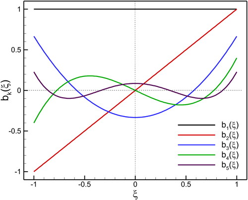denotes the total number of modal coefficients for l-th order accurate polynomials. In this work, hierarchical basis functions based on orthogonal scaled Legendre (modal) polynomials are used in the computational element $I_n=[-1,1]$ (Singh 2018). (4) $$\begin{array}{c}\begin{array}{c}{b}_i(\xi )=\frac{2^i{(i!)}^2}{(2i)!}{P}_i^{0,0}(\xi ),\hspace{1em}n\ge 0,\hfill \\ \xi =\frac{(x-x_i)}{\Delta x/2},\hspace{1em}-1\le \xi \le 1,\hfill \end{array}\hfill \end{array}$$(4) where $P_n^{0,0}(.)$ denotes the Legendre polynomials. The first five orthogonal scaled Legendre polynomials which corresponds to the fourth-order approximations are evaluated as follows. (5) $$\begin{array}{c}\begin{array}{c}{\phi }_1(\xi )=1,\hspace{1em}{\phi }_2(\xi )=\xi ,\hspace{1em}{\phi }_3(\xi )={\xi }^2-\frac{1}{3},\hfill \\ {\phi }_4(\xi )={\xi }^3-\frac{3}{5}\xi ,\hspace{1em}{\phi }_5(\xi )={\xi }^4-\frac{6}{7}{\xi }^2+\frac{3}{35},\hfill \end{array}\hfill \end{array}$$(5) which are illustrated in Figure 1

Figure 1. Visualization the modes of one-dimensional scaled Legendre basis polynomials corresponding to the 4th-order approximation.

For the spatial discretization of equation Equation (1)(1) $$\frac{\partial \mathbf{U}}{\partial t}+\frac{\partial \mathbf{F}(\mathbf{U})}{\partial x}=\mathbf{P}(\mathbf{U}),$$(1) , we establish the following weak formulation for ${\mathbf{U}}_h\in V_h^l(\mathfrak{I}),$ which is obtained by multiplying Equation (1)(1) $$\frac{\partial \mathbf{U}}{\partial t}+\frac{\partial \mathbf{F}(\mathbf{U})}{\partial x}=\mathbf{P}(\mathbf{U}),$$(1) by a test function $b_h,$ integrating over the domain ${\Omega }_e\in \mathfrak{I},$ and executing the integration by parts: (6) $$\begin{array}{c}\frac{\partial }{\partial t}\underset{{\Omega }_e}{\int }{\mathbf{U}}_h{b}_h \mathit{\text{dV}}+\underset{{\Omega }_e}{\int }\nabla b_h·\mathbf{F}({\mathbf{U}}_h)\mathit{\text{dV}}-\underset{\partial {\Omega }_e}{\int }{b}_h\mathbf{F}({\mathbf{U}}_h)·\mathbf{n} d\Gamma =\underset{{\Omega }_e}{\int }{b}_h \mathbf{P}({\mathbf{U}}_h)\mathit{\text{dV}}.\hfill \end{array}$$(6)

Here, $\mathbf{n}$ denotes the outward unit normal vector, while V and $\Gamma$ denote the volume and boundary of the element ${\Omega }_e,$ respectively. The numerical solution ${\mathbf{U}}_h$ is discontinuous across element interfaces, therefore the interface fluxes are not uniquely defined. The flux function $\mathbf{F}·\mathbf{n}$ appearing in Equation (6)(6) $$\begin{array}{c}\frac{\partial }{\partial t}\underset{{\Omega }_e}{\int }{\mathbf{U}}_h{b}_h \mathit{\text{dV}}+\underset{{\Omega }_e}{\int }\nabla b_h·\mathbf{F}({\mathbf{U}}_h)\mathit{\text{dV}}-\underset{\partial {\Omega }_e}{\int }{b}_h\mathbf{F}({\mathbf{U}}_h)·\mathbf{n} d\Gamma =\underset{{\Omega }_e}{\int }{b}_h \mathbf{P}({\mathbf{U}}_h)\mathit{\text{dV}}.\hfill \end{array}$$(6) is replaced by a single-valued function defined at the cell interfaces, the so-called numerical flux function represented as $\widehat{\mathbf{H}}.$ In present work, the local Lax-Friedrichs (LLF) flux is employed for the numerical flux. This monotone flux is commonly used in the DG method due to its efficiency in computational cost. (7) $$\begin{array}{c}\begin{array}{cc}\mathbf{F}·\mathbf{n}\equiv \widehat{\mathbf{H}}({\mathbf{U}}_h^{+},{\mathbf{U}}_h^{-})=\frac{1}{2}\left[\left(\mathbf{F}({\mathbf{U}}_h^{+})+\mathbf{F}({\mathbf{U}}_h^{-})\right)-C({\mathbf{U}}_h^{+}-{\mathbf{U}}_h^{-})\right],& \\ C=\mathrm{\text{max}}\left(\left|{\mathbf{U}}_h^{+}\right|+a_s^{+},\left|{\mathbf{U}}_h^{-}\right|+a_s^{-}\right),& \hfill \end{array}\end{array}$$(7) where $a_s^{\pm }=C_{\mathrm{\text{max}}} \sqrt{{(p/\rho )}^{\pm }}$ discusses the G13 speeds. In this notation, $C_{\mathrm{\text{max}}}$ is the maximum propagation speed in the kinetic moment model. For G13 model, $C_{\mathrm{\text{max}}}=1.6503$ (Torrilhon 2000, 2016). The superscripts $(-)$ and $(+)$ denote the left and right states of the element interface. Thus, the weak formulation (6)(6) $$\begin{array}{c}\frac{\partial }{\partial t}\underset{{\Omega }_e}{\int }{\mathbf{U}}_h{b}_h \mathit{\text{dV}}+\underset{{\Omega }_e}{\int }\nabla b_h·\mathbf{F}({\mathbf{U}}_h)\mathit{\text{dV}}-\underset{\partial {\Omega }_e}{\int }{b}_h\mathbf{F}({\mathbf{U}}_h)·\mathbf{n} d\Gamma =\underset{{\Omega }_e}{\int }{b}_h \mathbf{P}({\mathbf{U}}_h)\mathit{\text{dV}}.\hfill \end{array}$$(6) becomes, (8) $$\begin{array}{c}\frac{\partial }{\partial t}\underset{{\Omega }_e}{\int }{\mathbf{U}}_h{b}_h \mathit{\text{dV}}+\underset{{\Omega }_e}{\int }\nabla b_h·\mathbf{F}({\mathbf{U}}_h)\mathit{\text{dV}}-\underset{\partial {\Omega }_e}{\int }{b}_h \widehat{\mathbf{H}}({\mathbf{U}}_h)\hspace{0.17em}\hspace{0.17em}d\Gamma =\underset{{\Omega }_e}{\int }{b}_h \mathbf{P}({\mathbf{U}}_h)\mathit{\text{dV}}.\hfill \end{array}$$(8)

To solve the DG week formulation (8)(8) $$\begin{array}{c}\frac{\partial }{\partial t}\underset{{\Omega }_e}{\int }{\mathbf{U}}_h{b}_h \mathit{\text{dV}}+\underset{{\Omega }_e}{\int }\nabla b_h·\mathbf{F}({\mathbf{U}}_h)\mathit{\text{dV}}-\underset{\partial {\Omega }_e}{\int }{b}_h \widehat{\mathbf{H}}({\mathbf{U}}_h)\hspace{0.17em}\hspace{0.17em}d\Gamma =\underset{{\Omega }_e}{\int }{b}_h \mathbf{P}({\mathbf{U}}_h)\mathit{\text{dV}}.\hfill \end{array}$$(8) , the appearing volume and boundary integrals must be approximated. In this work, the Gauss-Legendre quadrature rule assesses the volume and boundary integrals within the elements and over the interfaces to ensure high order accuracy. These quadrature rules require the exact polynomials of degree 2 l and $2l+1$ for the numerical integrations inside the elements and over the interfaces, respectively (Cockburn and Shu 1998). In high-order numerical schemes, spurious numerical fluctuations of the solutions may result in negative density and pressure during the time evaluation, violating the physical constraint of positivity. Therefore, a positivity preserving limiter is needed to enforce positive pressure and density at every element. In this work, a positivity preserving limiter proposed by Zhang and Shu (2010) is employed.

Finally, by assembling all the elemental contributions together, the modal DG formulation leads to a semi-discrete system of ordinary differential equations in time, (9) $$\begin{array}{c}\mathbf{M}\frac{d\mathbf{U}}{\mathit{\text{dt}}}=\mathbf{L}(\mathbf{U}),\hfill \end{array}$$(9) where $\mathbf{M},$ and $\mathbf{L}(\mathbf{U})$ are the block diagonal mass matrix, and the residual vector, respectively. Due to the diagonal nature of the mass matrix, its inverse may be simply evaluated by hand for each element. An explicit third-order accurate strong stability preserving (SSP) Runge-Kutta method is used for time integration (Shu and Osher 1988). It has the form: (10) $$\begin{array}{c}\begin{array}{c}{\mathbf{U}}_h^{(1)}={\mathbf{U}}_h^n+\Delta t {\mathbf{M}}^{-1} \mathbf{L}(U_h^n),\hfill \\ {\mathbf{U}}_h^{(2)}=\frac{3}{4}{\mathbf{U}}_h^n+\frac{1}{4}{\mathbf{U}}_h^{(1)}+\frac{1}{4}\Delta t {\mathbf{M}}^{-1} \mathbf{L}(U_h^{(1)}),\hfill \\ {\mathbf{U}}_h^{n+1}=\frac{1}{3}{\mathbf{U}}_h^n+\frac{2}{3}{\mathbf{U}}_h^{(2)}+\frac{2}{3}\Delta t {\mathbf{M}}^{-1} \mathbf{L}({\mathbf{U}}_h^{(2)}),\hfill \end{array}\hfill \end{array}$$(10) where $\mathbf{L}(U_h^n)$ is the residual of approximate solutions at time $t_n,$ and $\Delta t$ is the suitable time-stepping length.

4. Accuracy and validation test for DG solver

To verify the order of accuracy of the numerical scheme, we consider a one-dimensional linear scalar problem: (11) $$\begin{array}{c}\begin{array}{c}\frac{\partial u}{\partial t}+\frac{\partial u}{\partial x}=0,\hspace{1em}x\in [0,2\pi ],\hfill \\ u(x,0)=\hspace{0.17em}\mathrm{\text{sin}}\hspace{0.17em}x,\hfill \end{array}\hfill \end{array}$$(11) with the periodic boundary condition $u(0,t)=u(2\pi ,t)$ and the exact solution $u(x,t)=\hspace{0.17em}\mathrm{\text{sin}}\hspace{0.17em}(x-t).$ The accuracy of the DG scheme is examined with four $P^1,P^2,P^3$ and $P^4$ elements. The errors $e_{\infty },$ $e_2$ and order (O) are measured as follows: (12) $$\begin{array}{c}\begin{array}{c}{e}_{\infty }=\mathrm{\text{max}}(|\widehat{u}(x,t)-u_h(x,t)|),\hfill \\ e_2=\sqrt{\sum _{I_n}{\int }_{I_n}|\widehat{u}(x,t)-u_h(x,t){|}^2}\mathit{\text{dx}},\hfill \\ O=\frac{\mathrm{\text{log}}((e(N_1)/e(N_2))}{\mathrm{\text{log}}(N_2/N_1)}\hfill \end{array}\hfill \end{array}$$(12) where $\widehat{u}(x,t)$ is the exact solution and $u_h(x,t)$ is the approximate solution. The $e(N_1)$ and $e(N_2)$ are the errors for N and 2 N elements, respectively. This problem is calculated up to $4^{\mathit{\text{th}}}$-order of accuracy at time $T_f=1$ by varying number of grid points $N(20,40,80,160).$ The numerical results for this problem with the order of accuracy in $e_2$ and $e_{\infty }$ are illustrated in Table 1. From the table, it is confirmed that the present numerical scheme achieves the desired order of accuracy $(l+1).$

Table 1. Accuracy test of the linear scalar problem.

l	N	$e_2$	O	$e_{\infty }$	O
1	20	$0.689292E-01$	−	$0.416916E-01$	$-$
	40	$0.179328E-01$	1.93	$0.106198E-01$	1.96
	80	$0.453598E-02$	1.97	$0.265698E-02$	2.01
	160	$0.113801E-02$	1.98	$0.663269E-03$	2.00
2	20	$0.104224E-02$	$-$	$0.124147E-02$	$-$
	40	$0.130558E-03$	3.03	$0.158800E-03$	2.95
	80	$0.163282E-04$	3.02	$0.200245E-04$	2.98
	160	$0.204129E-05$	3.01	$0.251331E-05$	2.99
3	20	$0.176257E-04$	$-$	$0.270453E-04$	$-$
	40	$0.110354E-05$	4.01	$0.170007E-05$	3.98
	80	$0.689895E-07$	4.03	$0.106066E-06$	3.99
	160	$0.431213E-08$	4.02	$0.662179E-08$	4.00
4	20	$0.252754E-06$	$-$	$0.429430E-06$	$-$
	40	$0.798519E-08$	5.05	$0.143225E-07$	4.92
	80	$0.246970E-09$	5.01	$0.444279E-09$	4.99
	160	$0.771945E-11$	5.03	$0.138960E-10$	5.01

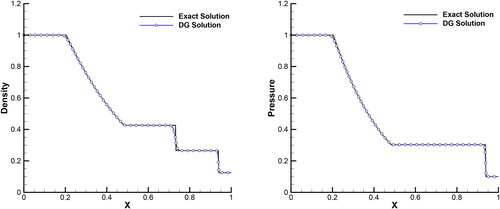
For validating the present DG solver, we also examine a classical Riemann problem based on the one-dimensional Euler equations associated with the Sod shock tube test. The initial conditions are described as (13) $$\begin{array}{c}(\rho ,u,p)=\{\begin{array}{cc}(1.0,0.0,1.0),\hfill & \text{if}x\le 0.5,\hfill \\ (0.125,0.0,0.1),\hfill & \text{if}x\ge \mathrm{0.5.}\hfill \end{array}\hfill \end{array}$$(13)

For this problem, the computational domain is considered as $D=[0,1],$ and the gas interface is positioned at $x=0.5.$ For the computational simulations, 400 grid points are used, while the zero gradient condition is employed at boundaries. Figure 2 illustrates the comparison of density and pressure distributions between the exact and numerical data. We observed that the solutions of these Riemann problems are in good agreement with the exact solution.

Figure 2. Validation of numerical solver: comparison of exact and numerical solutions for the calculated quantities (a) density and (b) pressure at $t=0.2$ in classical Sod shock tube problem.

5. Numerical experiments of G13 system in continuum-rarefied flow regime

In this section, we present the numerical experiments of G13 system in continuum-rarefied flow regime. For this purpose, we consider the one-dimensional Riemann problem with varying initial conditions, including shock tube,

5.1. Shock tube problem

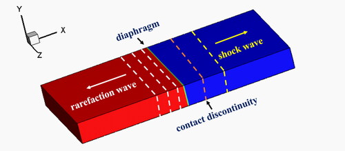
A shock tube is a special case of the Riemann problem in which the compressible gas is constant but of different state left and right of a diaphragm. Figure 3 gives a graphical representation of the Riemann problem at the initial state. This setup has strong density and pressure differences with zero velocity, causing a right-going shock wave, a left-going expansion fan (i.e., rarefaction wave), and a right-going contact discontinuity separating the shock wave and the expansion fan (Sod 1978).

Figure 3. Graphical representation and initial configuration of shock tube problem.

In this test case, we consider the Riemann problem for the G13 moment equations, which is a dissipative extension of the Euler case. The following initial conditions are considered for numerical experiments (14) $$\begin{array}{c}(\rho ,u,p,\sigma ,q)=\{\begin{array}{cc}({\rho }_1,0,p_1,0,0),\hfill & \text{if}x\le 0.5,\hfill \\ ({\rho }_0,0,p_0,0,0),\hfill & \text{if}x\ge \mathrm{0.5.}\hfill \end{array}\hfill \end{array}$$(14)

With these conditions, we solve the G5 and G13 systems. As reference state, the low pressure state ${\rho }_0,p_0$ is chosen. The pressure and density ratios are considered as (15) $$\frac{p_1}{p_0}=\frac{{\rho }_1}{{\rho }_0}=5,$$(15) such that temperature is constant.

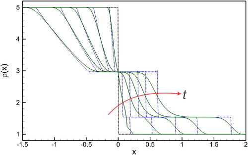
Figure 4 illustrates the time evolution of density profiles for G5 and G13 equations at a fixed Knudsen number $\mathit{\text{Kn}}=0.01.$ We can see from the density plots that the G13 solution follows the profiles of the G5 solution in a diffusive way after a startup phase. Because of finite Kn number appearing in G13 system, these diffusive profiles have a stronger physical relevance than the discontinuities in the Euler case. Interestingly, we are able to resolve the shock’s diffusive structure with increasing the value of Kn number. Only when $\mathit{\text{Kn}}\to 0$ does the Euler equations hold, and in that scenario the discontinuity represents the shock structure. A traveling wave formed by the shock structure can be computed independently. Because of heat conduction, the contact discontinuity profile is not constant; rather, it smears out slowly over time.

Figure 4. Time evolution of density profiles for G13 (solid line), and G5 equations (dashed line) at Kn $=0.01.$

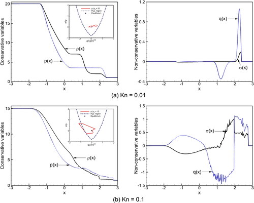
Figure 5 shows the Kn number effect on the behavior of macroscopic quantities: density ($\rho$), pressure (p), velocity (v), temperature ($\theta$), stress ($\sigma$), and heatflux (q) in G5 and G13 systems for a fixed time. We run the simulations till $t=0.35$ over the computational domain $[-1,1]$ with 500 grid points. Because of its self similarity, the solution to G5 system can be seen to exhibit the same shape at any Kn value. Since the scale for time and space is infinitesimally small, the G13 system approximates the collisionless region. Therefore, we are able to solve the Riemann problem of the G13 system (1)(1) $$\frac{\partial \mathbf{U}}{\partial t}+\frac{\partial \mathbf{F}(\mathbf{U})}{\partial x}=\mathbf{P}(\mathbf{U}),$$(1) . The solutions have five characteristic waves according to the five characteristic velocities, including two rarefaction waves and three discontinuities (Torrilhon 2000). For large Kn number, the solutions of G13 system bear absolutely no similarities to the G5 system. The discontinuities in the G13 system lose their strength and the rarefaction waves become smoother as a result of dissipation. Once more, it is evident that when discontinuities are damped, they slow down. In Figure 5, the G13 system recognizes the propagation of the contact discontinuity as well as of the rarefaction wave, which move according to the characteristics of the G5 system, although these characteristics are absent in the G13 system. 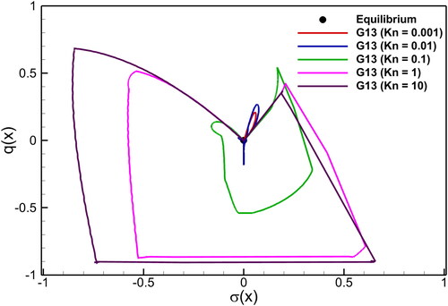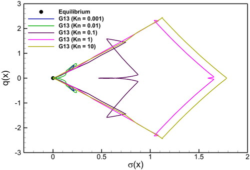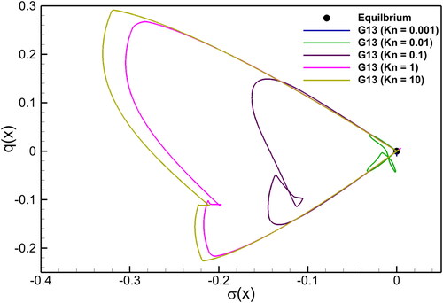In stress ($\sigma$) and heat flux (q), five characteristic waves are found in the starting. At higher Kn, sub-shocks are also observed. In such waves, shock speeds are faster than the characteristic speeds in the G13 system. The non-monotone form of the gradual rarefaction wave in the stress is remarkable. These waves are damped, and the outcome is soliton-like solutions, which show that there is non-equilibrium across the contact discontinuities, the shock structures, and -much less—across the rarefaction wave. Figure 6 illustrates the Kn effects on the shock tube solutions through normal stress vs heat flux in the G13 system at $t=0.35.$ It is evident that when Kn increases, the degree of non-equilibrium enhances as well, indicating a significant deviate from the local equilibrium state.

Figure 5. Shock tube problem: Kn number effect on macroscopic quantities (density ($\rho$), pressure (p), velocity (v), temperature ($\theta$), stress ($\sigma$), and heat flux (q)) in the G5 and G13 systems at $t=0.35.$

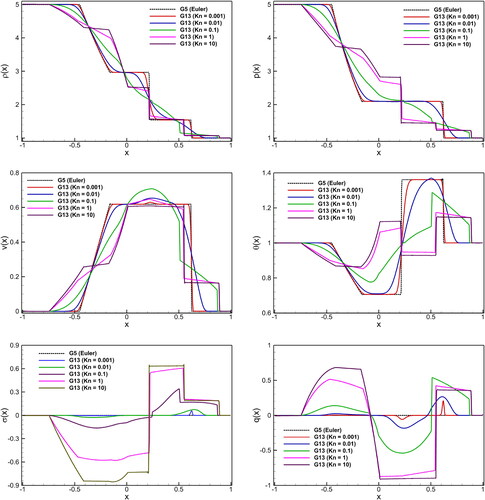
Figure 6. Shock tube problem: Kn number effect on the solutions of normal stress vs heat flux in the G13 system at $t=0.35.$

Furthermore, the Kn number effect on the spatiotemporal contours for density ($\rho$), pressure $(p)$ and heat flux (q) solutions in the G5 and G13 systems can be illustrated in Figures 7–9. These figures show the fields as function of space and time simultaneously. The $x-$ axis represents the spatial interval [−4,4], while time evolves along the $y-$ axis. At $t=0,$ the initial condition is visible along the $x-$ axis and Figures 7 and 8 show only two colors for the initial left- and right-hand state of density and pressure, respectively. The upper left plot of the figures shows the result of the Euler equations. There, the contours clearly indicate the shock wave and contact discontinuity as well as the smooth variation of the fields across the rarefaction fan. The middle plot in the upper row shows the result of the G13 equations based on a very small $\mathit{\text{Kn}}-$ number. The small value of Kn implies large scales for the space and time axes and the contours are virtually indistinguishable from the Euler result. We now zoom into the area around the origin of the plot (see the indicated white box) in order to see the build-up of the shock tube solution. For the Euler result this zoom would not change the picture, however, the G13 result allows to investigate these small scales. The plot in the upper right corner of the figure represents the zoomed-up area around the origin of the previous plot. This is equivalent to increasing the Kn number by a factor of ten, such that the axes of time and space display smaller scales. Both contact and shock begin to smear out. The lower left plot shows another zoom of the previous plot around the origin by a factor 10. Rarefaction, contact and shock merge into a completely different wave pattern which becomes fully visible by successive zooming in the two remaining plots of the figure. This metamorphosis is most visible in the pressure contours of Figure 8, where the single intermediate pressure state in blue color, gives way to five waves (three discontinuities and two rarefactions) in the maximal zoom. Note that the G13 equations loose physical validity for Kn numbers larger the 0.1. The wave patterns in the zoomed result for larger Kn numbers are a rough approximation of the free-flight behavior of the gas at very short times in a shock tube experiment [see Au, Torrilhon, and Weiss (2001)].

Figure 7. Kn number effect on the spatiotemporal contours for density solution in the G5 and G13 systems. In each sub-figure, horizontal axis denotes the $x\in [-4.0,4.0],$ while vertical axis represents the time $t\in [0,1.5].$

Figure 8. Kn number effect on the spatiotemporal contours for pressure solution in the G5 and G13 systems. In each sub-figure, horizontal axis denotes the $x\in [-4.0,4.0],$ while vertical axis represents the time $t\in [0,1.5].$

Figure 9. Kn number effect on the spatiotemporal contours for heat flux solution in the G5 and G13 systems. In each sub-figure, horizontal axis denotes the $x\in [-4.0,4.0],$ while vertical axis represents the time $t\in [0,1.5].$

Figure 9 shows the contours of the space-time result of the heat flux. As the Euler equations cannot predict heat flux the upper left plot of the figure shows the homogeneous color of a zero solution. This can be compared to a large scale solution of G13 in the middle plot of the upper row. Here, two very fine lines indicate non-vanishing heat fluxes inside the contact and the shock. Zooming into this result reveals thicker contact and shock wave in the upper right plot and also some heat flux around the rarefaction wave. The wave pattern then changes dramatically in the next zoom of the lower left plot. Large value of heat flux indicate a strong dissipation mechanism in the build-up phase of the shock tube solution. The final zoom in the lower right corner again displays the artificial waves of G13 which can be mapped to the waves visible in density and pressure in Figures 8 and 9.

The G13 moment equations are not globally hyperbolic, due to linearization during the derivation of the system. For a given equilibrium state $\rho ,$ p only a certain range of values of stress ($\sigma$) and heatflux (q) close to equilibrium are allowed. The characteristic polynomial of the G13 system has imaginary roots outside this range (Torrilhon 2000). If the stress and heat flux are made dimensionless with the specified equilibrium conditions: (16) $$\begin{array}{c}\overline{\sigma }=\frac{\sigma }{p},\overline{q}=\frac{q}{p\sqrt{\frac{p}{q}}}=\frac{q}{\rho {\theta }^{3/2}},\text{with} p=\rho \theta .\hfill \end{array}$$(16)

Now, we can draw a region of hyperbolicity in the $(\overline{\sigma },\overline{q})$-plane. The borderline of the region of hyperbolicity is given by the following mathematical relationship, see Müller and Ruggeri (1998). (17) $$\overline{q}(\overline{\sigma })=\pm \frac{1}{972}\sqrt{\frac{5}{3}}(117+93\overline{\sigma }-D(\overline{\sigma }))\sqrt{117+93\overline{\sigma }+2D(\overline{\sigma })},$$(17) with (18) $$D(\overline{\sigma })=\sqrt{8541{\overline{\sigma }}^2+14553\overline{\sigma }+\frac{15957}{2}}.$$(18)

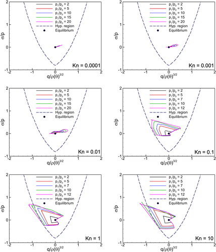
Figure 10 illustrates the solutions of G13 systems for the Riemann problem (14)(14) $$\begin{array}{c}(\rho ,u,p,\sigma ,q)=\{\begin{array}{cc}({\rho }_1,0,p_1,0,0),\hfill & \text{if}x\le 0.5,\hfill \\ ({\rho }_0,0,p_0,0,0),\hfill & \text{if}x\ge \mathrm{0.5.}\hfill \end{array}\hfill \end{array}$$(14) with different density/pressure ratios ($p_1/p_0={\rho }_1/{\rho }_0=2,5,7,10,12,15,20$) with varying Kn. The same density and pressure ratio lead to a constant initial temperature through the relation $\theta =p/\rho .$ In this figure, the hyperbolicity boundary is shown by dashed lines, and the equilibrium state ($\sigma =q=0$) is given by black dot point. It is noteworthy that hyperbolicity is given for not too large heat fluxes and not too small stress values. For large values of the heat flux and for very small values of $\sigma /p$ hyperbolicity is lost. A polygon with five legs, representing the five characteristic waves, is observed for greater Kn values, that is, $\mathit{\text{Kn}}=10.$ As Kn number decreases, the polygon collapses due to the damping. Consequently, a small steady loop is formed, which indicates mainly the dissipation in the shock structure. It is also observed that with increasing the values of $p_1/p_0$ as well as Kn number, the $\sigma -q$ curves leaves the hyperbolicity region. In this instance, the G13 system loses its hyperbolicity and turns unstable, resulting in the nonphysical solutions.

Figure 10. Kn number effect on the several solutions of the G13 system with different pressure ratios in the hyperbolicity region.

To demonstrate the influence of this loss of hyperbolicity, a shock tube problem with two different $p_1/p_0={\rho }_1/{\rho }_0$ ratios is considered. Figure 11 illustrates the four macroscopic quantities ($\rho ,p,\sigma ,q$) for G13 system at two different Kn numbers. In Figure 11a, the initial density and pressure ratio is 20 with $\mathit{\text{Kn}}=0.01,$ while in Figure 11b, the ratio is 15 with $\mathit{\text{Kn}}=0.1.$ It can be observed that at $\mathit{\text{Kn}}=0.01$ and $p_1/p_0=20,$ the $\sigma -q$ curve of G13 system lies inside the hyperbolicity region, thus, the smooth and physical solutions are obtained. On the other hand, at $\mathit{\text{Kn}}=0.1,$ $\sigma -q$ curve of G13 system goes out from the hyperbolicity region, thus, the oscillated and nonphysical solutions are obtained.

Figure 11. Hyperbolicity boundary and two different initial conditions for G13 system. For pressure ratio of 15, the ellipticity of G13 equations leads to oscillations and break-down of the computation.

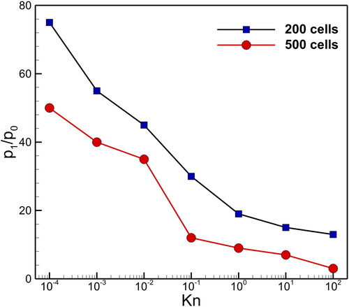
Figure 12 displays the profiles for pressure ratio ($p_1/p_0$) vs Kn number in the shock tube problem with two different numbers of cells i.e., 200 and 500 cells. This figure represents the robustness of the current numerical scheme. The calculations for these profiles are performed with $4^{\mathit{\text{th}}}$-order DG approximations in the computational domain [-2,2]. The current number scheme readily converges to $p_1/p_0=50$ at $\mathit{\text{Kn}}={10}^{-4}$ with 500 cells, and to 3 at $\mathit{\text{Kn}}=100.$ With less cells, say 200, this pressure ratio increases with Kn numbers.

Figure 12. Shock tube problem: profile for pressure ratio vs Kn number.

5.2. Two shock waves

This section considers another Riemann problem with two shock waves moving away from each other. We consider the domain $[-0.5,0.5]$ with outflow boundary conditions. The initial discontinuity is centered at $x=0,$ separating the left and right states given below. (19) $$\begin{array}{c}(\rho ,u,p,\sigma ,q)=\{\begin{array}{cc}(1.0,1.0,1.0,0,0),\hfill & \text{if}x\le 0.5,\hfill \\ (1.0,-1.0,1.0,0,0),\hfill & \text{if}x\ge \mathrm{0.5.}\hfill \end{array}\hfill \end{array}$$(19)

Figure 13 illustrates the Kn number effect on the behavior of macroscopic quantities, including density ($\rho$), pressure (p), velocity (v), temperature ($\theta$), stress ($\sigma$), and heatflux (q) in the G5 and G13 systems. All the solutions are based on calculations done at $t=0.125.$ These simulations are done with 500 cells and $4^{\mathit{\text{th}}}$ order DG approximation. The G5 system solution has the same shape at any Kn value due to its self-similarity. The G13 system approximates the collisionless region because time and space are infinitesimally small. Therefore, G13 solutions are completely different from the G5 solutions for large Kn numbers. An interesting result is that as Kn rises, so does the degree of non-equilibrium, indicating a large deviation from local equilibrium, as illustrated in Figure 14.

Figure 13. Two shock waves: Kn effects on macroscopic quantities in the G5 and G13 systems at $t=0.125.$

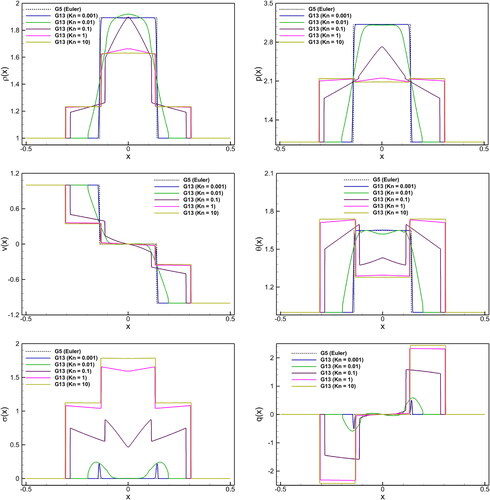
Figure 14. Two shock waves: Kn effects on the solutions of normal stress vs heat flux in the G13 system at $t=0.125.$

5.3. Two rarefaction waves

In the last test case, we consider a Riemann problem with two rarefaction waves. The following is the initial condition for this problem in the calculation domain $[-0.5,0.5]:$ (20) $$\begin{array}{c}(\rho ,u,p,\sigma ,q)=\{\begin{array}{cc}(2.0,-0.5,1.5,0,0),\hfill & \text{if}x\le 0.5,\hfill \\ (1.0,0.5,1.0,0,0),\hfill & \text{if}x\ge \mathrm{0.5.}\hfill \end{array}\hfill \end{array}$$(20)

For the numerical simulations, we use outflow boundary conditions, and the solutions are computed until time $t=0.15$ using 500 cells. Five quadrature points and a $4^{\mathit{\text{th}}}$ order DG approximation are used in all simulations. Figure 15 displays the Kn impacts on the behavior of primitive and non-primitive quantities in the G5 and G13 systems such as density ($\rho$), pressure (p), velocity (v), temperature ($\theta$), stress ($\sigma$), and heatflux (q). Similar to the previous two test cases, the G13 solutions become smooth with increasing Kn number. Further, Figure 16 show profiles of the non-conserved variables (viscous stress and heat flux). This figure clearly shows that the profiles of two rarefaction waves is not symmetrical in the phase space of the non-conserved variables. A higher Kn number corresponds to larger non-conserved variable magnitudes.

Figure 15. Two rarefaction waves: Kn effect on macroscopic quantities in the G5 and G13 systems at $t=0.15.$

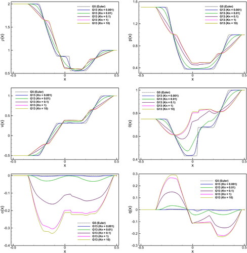
Figure 16. Two rarefaction waves: Kn effects on the solutions of nomral stress vs heat flux in the G13 system at $t=0.15.$

6. Concluding remarks and outlook

In this study, we present the numerical simulations of G13 moment equations with application to the Riemann problem in a wide range of continuum-rarefied flow regimes. Here, we emphasize the numerical robustness and wave phenomena in the G13 system to provide a building block for R13 system and high-order Grad’s models. For this purpose, a high-order modal discontinuous Galerkin solver is employed for solving one-dimensional G13 moment equations. For spatial discretization, hierarchical modal basis functions premised on orthogonal scaled Legendre polynomials are used. The proposed approach reduces the G13 systems into a framework of ordinary differential equations in time, which are addressed by an explicit third-order SSP Runge-Kutta algorithm. We verify the reliability and accuracy of the used numerical solver by comparing the current results with a classical Riemann problem’s results, which show a good degree of agreement. Three Riemann test problems, including shock tube problem, two shock waves, and two rarefaction waves are examined in continuum-rarefied flow regime. The numerical results demonstrate that every Riemann problem has not a solution for the G13 system because of loss of hyperbolicity of the system.

The main objective of this paper is to provide a systematic DG framework for simulating one-dimensional G13 moment system in a wide range of continuum-rarefied flow regime. This DG framework can be easily extended to multidimensional G13 and R13 moment systems with various interesting applications, such as shocked hydrodynamic instability, shock-vortex interaction, etc. In this context, we hope to report the numerical results of multidimensional G13 moment systems for these applications in the future.

Disclosure statement

No potential conflict of interest was reported by the author(s).

Additional information

Funding

The authors acknowledge funding through the German Research Foundation within the Research unit DFG–FOR5409.

Appendix:

A grid convergence study

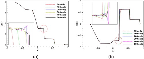
In order to predict the correct flow physics of G13 system, a grid convergence study for shock tube problem is conducted at a higher Kn number, i.e., $\mathit{\text{Kn}}=1.$ For this purpose, Figure A1 shows the density and heat flux solutions on six different grids, including 50, 100, 200, 300, 400 and 500 cells. Here, the numerical simulations are performed with $4^{\mathit{\text{th}}}$ order DG approximation and 5 quadrature points. These grids are used to compare the effects of mesh resolutions on the numerical solutions. As expected, the accuracy of the solution improves with finer grids. Therefore, 500 cells are used to assure numerical accuracy in the considered test cases.

Figure A1. Grid convergence study in shock tube problem at Kn = 1: profiles of (a) density, and (b) heat flux quantities for six different cells.

References

- Au, J. D., M. Torrilhon, and W. Weiss. 2001. A survey of several finite difference methods for systems of nonlinear hyperbolic conservation laws. Phys. Fluids 13 (8):2423–32. doi: 10.1063/1.1381018
- Cercignani, C. 1975. Theory and application of the Boltzmann equation. Cambridge: Oxford University Press.
- Chan, J., Y. Lin, and T. Warburton. 2022. Entropy stable modal discontinuous Galerkin schemes and wall boundary conditions for the compressible Navier-Stokes equations. Comput. Phys. 448:110723. doi: 10.1016/j.jcp.2021.110723
- Cockburn, B., and C.-W. Shu. 1998. The Runge–Kutta discontinuous Galerkin method for conservation laws V: Multidimensional systems. Comput. Phys. 141 (2):199–224. doi: 10.1006/jcph.1998.5892
- Ellefson, R., and A. Miiller. 2000. Recommended practice for calibrating vacuum gauges of the thermal conductivity type. J. Vac. Sci. Technol. A: Vac. Surf. Films 18 (5):2568–77. doi: 10.1116/1.1286024
- Gad-el-Hak, M. 2005. The MEMS handbook: Introduction and fundamentals. Boca Raton: CRC Press.
- Gassner, G. J., A. R. Winters, and D. A. Kopriva. 2016. Split form nodal discontinuous Galerkin schemes with summation-by-parts property for the compressible Euler equations. Comput. Phys. 327:39–66. doi: 10.1016/j.jcp.2016.09.013
- Grad, H. 1949. On the kinetic theory of rarefied gases. Comm. Pure Appl. Math. 2 (4):331–407. doi: 10.1002/cpa.3160020403
- Hesthaven, J. S., and T. Warburton. 2007. Nodal discontinuous Galerkin methods: Algorithms, analysis, and applications. New York: Springer Science & Business Media.
- Hindenlang, F., G. J. Gassner, C. Altmann, A. Beck, M. Staudenmaier, and C. Munz. 2012. Explicit discontinuous Galerkin methods for unsteady problems. Comput. Fluids 61:86–93. doi: 10.1016/j.compfluid.2012.03.006
- Jou, D., J. Casas-Vazquez, and G. Lebon. 1996. Extended irreversible thermodynamics. 2nd ed. Berlin: Springer-Verlag Press.
- Karniadakis, G. M., and A. Beskok. 2002. Micro flows: Fundamentals and simulation. Oxford: Oxford University Press.
- Kontzialis, K., and J. A. Ekaterinaris. 2013. High order discontinuous Galerkin discretizations with a new limiting approach and positivity preservation for strong moving shocks. Comput. Fluids 71:98–112. doi: 10.1016/j.compfluid.2012.10.009
- Kronbichler, M., and W. A. Wall. 2018. A performance comparison of continuous and discontinuous Galerkin methods with fast multigrid solvers. SIAM J. Sci. Comput. 40 (5):A3423–A3448. doi: 10.1137/16M110455X
- Müller, I., and T. Ruggeri. 1998. Rational extended thermodynamics. 2nd ed. New York: Springer Tracts in Natural Philosophy, Springer.
- Raj, L. P., S. Singh, A. Karchani, and R. S. Myong. 2017. A super-parallel mixed explicit discontinuous Galerkin method for the second-order Boltzmann-based constitutive models of rarefied and microscale gases. Comput. Fluids 157:146–63. doi: 10.1016/j.compfluid.2017.08.026
- Rana, A., M. Torrilhon, and H. Struchtrup. 2013. A robust numerical method for the R13 equations of rarefied gas dynamics: Application to lid driven cavity. Comput. Phys. 236:169–86. doi: 10.1016/j.jcp.2012.11.023
- Reed, W. H., and T. R. Hill. 1973. Triangular mesh methods for the neutron transport equation. Los Alamos, NM: Los Alamos Scientific Lab.
- Reese, J. M., M. A. Gallis, and D. A. Lockerby. 2003. New directions in fluid dynamics: Non-equilibrium aerodynamic and microsystem flows. Philos. Trans. A Math. Phys. Eng. Sci. 361 (1813):2967–88. doi: 10.1098/rsta.2003.1281
- Shu, C. W., and S. Osher. 1988. Efficient implementation of essentially non-oscillatory shock-capturing schemes. Comput. Phys. 77 (2):439–71. doi: 10.1016/0021-9991(88)90177-5
- Singh, S. 2018. Development of a 3D discontinuous Galerkin method for the second-order Boltzmann-Curtiss based hydrodynamic models of diatomic and polyatomic gases. PhD diss., Gyeongsang National University.
- Singh, S., A. Karchani, and R. S. Myong. 2018. Non-equilibrium effects of diatomic and polyatomic gases on the shock-vortex interaction based on the second-order constitutive model of the Boltzmann-Curtiss equation. Phys. Fluids 30 (1):016109. doi: 10.1063/1.5009122
- Singh, S., A. Karchani, T. Chourushi, and R. S. Myong. 2022. A three-dimensional modal discontinuous Galerkin method for the second-order Boltzmann-Curtiss-based constitutive model of rarefied and microscale gas flows. Comput. Phys. 457:111052. doi: 10.1016/j.jcp.2022.111052
- Singh, S., and M. Battiato. 2020. Strongly out-of-equilibrium simulations for electron Boltzmann transport equation using modal discontinuous Galerkin approach. Int. J. Appl. Comput. Math. 6 (5):1–17. doi: 10.1007/s40819-020-00887-2
- Singh, S., and M. Battiato. 2021. An explicit modal discontinuous Galerkin method for Boltzmann transport equation under electronic nonequilibrium conditions. Comput. Fluids 224:104972. doi: 10.1016/j.compfluid.2021.104972
- Singh, S., R. C. Mittal, S. R. Thottoli, and M. Tamsir. 2023. High-fidelity simulations for Turing pattern formation in multi-dimensional Gray–Scott reaction-diffusion system. Appl. Math. Comput. 452:128079. doi: 10.1016/j.amc.2023.128079
- Sod, G. A. 1978. A survey of several finite difference methods for systems of nonlinear hyperbolic conservation laws. Comput. Phys. 27 (1):1–31. doi: 10.1016/0021-9991(78)90023-2
- Struchtrup, H. 2005. Macroscopic transport equations for rarefied gas flows. Berlin, Heidelberg: Springer Press.
- Struchtrup, H., and M. Torrilhon. 2003. Regularization of Grad’s 13 moment equations: Derivation and linear analysis. Physics of Fluids 15 (9):2668–80. doi: 10.1063/1.1597472
- Torrilhon, M. 2000. Characteristic waves and dissipation in the 13-moment-case. Continuum Mech. Thermodyn. 12 (5):289–301. doi: 10.1007/s001610050138
- Torrilhon, M. 2006. Two-dimensional bulk microflow simulations based on regularized Grad’s 13-moment equations. Multiscale Model. Simul. 5 (3):695–728. doi: 10.1137/050635444
- Torrilhon, M. 2016. Modeling nonequilibrium gas flow based on moment equations. Annu. Rev. Fluid Mech. 48 (1):429–58. doi: 10.1146/annurev-fluid-122414-034259
- Torrilhon, M., and H. Struchtrup. 2004. Regularized 13-moment equations: Shock structure calculations and comparison to Burnett models. J. Fluid Mech. 513:171–98. doi: 10.1017/S0022112004009917
- Vincenti, W. G., and C. H. Kruger. 1965. Introduction to physical gas dynamics. New York: Wiley Press.
- Xiao, H., and Q. J. He. 2018. Aero-heating in hypersonic continuum and rarefied gas flows. Aerosp. Sci. Technol. 82-83:566–74. doi: 10.1016/j.ast.2018.09.036
- Zhang, X., and C. W. Shu. 2010. On positivity-preserving high order discontinuous Galerkin schemes for compressible Euler equations on rectangular meshes. Comput. Phys. 229 (23):8918–34. doi: 10.1016/j.jcp.2010.08.016