JCARP: Joint Channel Assignment and Routing Protocol for cognitive-radio-based internet of things (CRIoT)

ABSTRACT

To deal efficiently with the spectrum sharing between cognitive radio users, we propose an innovative routing protocol involving not only a joint and fully distributed spectrum management, but also a hybridization mechanism, titled as Joint Channel Assignment and Routing Protocol (JCARP). Interestingly, it does not require a central control entity and does not use a common control channel to handle the network's spectrum distribution information. Additionally, in the route discovery phase of the hybrid routing protocol, there are two phases: reactive channel selection and proactive channel selection. Moreover, Secondary Users (SUs) have the option of switching from the reactive to the proactive phase of channel selection by utilizing historical usage information related to their list of available channels that has been stored in their database tables. In particular, carrier sense multiple access with collision avoidance transmission effects (pass or collision) are studied to identify channel availability and utilization, which are then fed into a database table pertaining to each SU. The JCARP protocol's performance is assessed through a Java–based simulator, utilizing throughput as the evaluation metric. The simulation results indicate that the JCARP protocol markedly reduces collisions among SUs during spectrum access opportunities in the transmission process, achieving higher throughput compared to its counterparts' protocols.

KEYWORDS:

• Cognitive radio network
• carrier sense multiple access with collision avoidance
• reactive channel selection
• proactive channel selection
• routing

1. Introduction

The Internet of Things (IoT) is a network of interconnected digital items that enables objects to communicate with one another and with computers without direct human or computer-to-human contact. The IoT concept has quickly developed to affect the majority of our everyday lives. However, because of its rapid growth, a spectrum must be found for the packets generated by IoT networks (Li et al., 2020; Nayyar, 2018). As a result, Cognitive Radio Networks (CRNs), also known as the CRIoT, were created to be integrated with the IoT idea (Bany Salameh et al., 2019; Darabkh, Awawdeh, et al., 2022; Singh & Moh, 2016). The CRN exists in two different architectural types: infrastructure (or centralized) and infrastructure-less (or dispersed) networks. Secondary users (SUs) in an infrastructure CRN rely on the base station to communicate and organize SUs’ communication. CR Ad-Hoc Network (CRAHN) is an alternative name for the infrastructure-less CRN (Li et al., 2020). An AHN that incorporates CR characteristics into a traditional AHN is called a CRAHN. As a consequence of the Primary Users’ (PU) activities involving various features, including a multi-hop architecture, the SUs must cooperate by sharing vital information about spectrum possibilities (i.e. time and place fluctuating) due to the absence of a centralized control entity (Bany Salameh et al., 2019; Darabkh, Khazaleh, et al., 2022; Singh & Moh, 2016). Moreover, CRAHNs’ varying topologies, spectrum heterogeneity, energy limitation, and self-organization are the challenging features that make CRAHNs a very motivating area for many interested researchers (Singh & Moh, 2016). While many researchers pay attention to spectrum sensing and sharing techniques, routing remains an important area to be explored in CRAHNs (Darabkh, Awawdeh, et al., 2023; Pourpeighambar et al., 2019).

PUs in CRNs typically refer to licensed entities, such as television broadcasters or wireless microphone users, holding primary access rights to specific frequency bands (Fernando & Lăzăroiu, 2023). In contrast, SUs are unlicensed entities that opportunistically access the spectrum during periods when PUs are not utilizing their allocated frequencies, leading to the emergence of spectrum holes (i.e. vacant licensed bands) (Muzaffar & Sharqi, 2024). The fundamental purpose of PUs in CRNs is to efficiently utilize their licensed spectrum while minimizing interference from unlicensed users. CR is often referred to as the SU of the spectrum (Zheng et al., 2023). In this context, CR is granted the privilege to utilize the unoccupied portion of the spectrum specifically when it becomes available due to the absence of the PU. SUs, who are also identified as unlicensed spectrum users, on the other hand, aim to exploit available spectrum opportunities opportunistically, enhancing spectrum utilization and addressing the challenge of spectrum scarcity (Teekaraman et al., 2023). The coexistence of PUs and SUs in CRNs facilitates improved spectral efficiency, providing a flexible and adaptive framework for wireless communication in dynamic and heterogeneous environments (Alqahtani et al., 2023).

Notably, routing protocols developed for different wireless networks cannot be applied for CRAHNs since they would significantly reduce protocol performance (Darabkh, Al-Khazaleh, et al., 2023; Malik et al., 2022). In other words, routing in heterogeneous and dynamic networks such as CRAHNs is far more complex than in stationary networks in many aspects. For example: (1) As a result of unexpected mobility of nodes which causes the dynamic nature of network topologies, frequent route failures occur. Similarly, (2) the list of channels that are available for a node differs not just over time (temporally) but also from node to node (spatially). (3) An SU is forced to leave the present channel and transition to another available one because of the abrupt entrance of the PU. Because of the variability in spectrum and routes caused by PU activity and node mobility, efficient routing circumstances are exacerbated. Routing, which in all types of wireless networks refers to the process of establishing a route between a source and a destination via intermediate nodes, is different in CRNs due to the requirement of locating available channels as well as intermediate CR nodes at each hop (Khasawneh et al., 2023).

Routing is essentially the foundation of communications, hence a strong routing protocol should also have a dependable channel selection process. Building stronger and more reliable routes is also made easier by the example channel selection techniques. These techniques opt for channels with extended availability periods, minimal interference for PUs, and reduced conflicts among SUs. Because of this, the cross-layer approach is an effective way to enhance routing algorithms in dynamic networks (Che-aron et al., 2014; Raj et al., 2020; Salih et al., 2023). In particular, a cross-layer design that integrates dynamic routing protocol with joint spectrum management (or channel assignment) is a desirable option; thus, cooperation between path selection and spectrum decision should be taken into account (Bany Salameh et al., 2020; Che-aron et al., 2014; Musa et al., 2020; Raj et al., 2020).

The influence of PU activity and the number of available channels for SUs has been the topics of prior studies. Nevertheless, spectrum sharing (i.e. the competition of SUs to access the spectrum holes or channels) takes limited attention. Majorly, to coordinate the access to the channels between the SUs, a Common Control Channel (CCC) is employed. Nevertheless, using CCC has many additional challenges, such as CCC coverage area, CCC saturation, CCC security, and robustness against PU’s activity (Hu et al., 2018; Lo, 2011). Besides, collisions can occur between SUs packets because of the competition to access the available spectrum holes.

As a result, SUs must share (access) the spectrum in an entirely distributed way, without using any form of CCC, such as dedicated unlicensed or licensed CCC, time-slotted CCC, or common hopping. Furthermore, the coordination between the SUs should remain in a tight range (i.e. without exchanging organization messages). That is an important point that must be considered when aiming to design a dynamic routing protocol and a fully distributed joint spectrum management and to achieve better performance and enhance the efficacy of CRNs. Additionally, there is a necessity for applying a suitable algorithm to organize the spectrum sharing between SUs for the sake of decreasing collisions.

On the other hand, an efficient routing algorithm with effective routing metrics should follow the spectrum management step, which is another challenge. Demonstrably, these applied routing metrics can accurately account for the quality of different paths to find the optimal route for data transmission (Khurana & Upadhyaya, 2019; Raj et al., 2020). Practically, the current wireless routing protocols cannot be immediately applied in CRNs, as these protocols degrade the overall efficiency and cause failures in CRNs. Moreover, the routing protocols are divided into three categories (Roy & Zade, 2018): Proactive or table-driven routing protocol, Reactive (or on-demand) routing protocol, and Hybrid routing protocol.

To discover routes to the destination, a reactive (or on-demand) routing protocol sends a large number of Route Request Packets (RRQPs) across the network, which might result in overhead and prolonged delay due to the fact that route discovery process is repeated in order to satisfy the uncertainty in the spectrum (Al-Rokabi & Politis, 2014). Additionally, the proactive (or table-driven) routing protocol creates a list of destinations and routes (tables of ready pathways). Following this, in order to maintain their currency, those tables are sporadically dispersed over the network. This results in a significant overhead because of the frequent table exchanges and the time needed to adjust to modifications in the network. Therefore, when updated appropriately, utilizing the hybrid protocol, incorporating the advantages of the prior protocols, will enhance network performance (Dutta & Sarma, 2023; Elrhareg et al., 2019; Salih et al., 2020).

This paper introduces an innovative routing protocol that integrates a fully distributed spectrum management (without CCC or neighbours table) with a hybrid routing protocol (hybrid channel selection) for CRAHNs, namely Joint Channel Assignment and Routing Protocol (JCARP). Initially, because JCARP is a fully distributed algorithm, we eliminate the CCC between SUs and neighbour tables to ensure that the cooperation between SUs is kept to a minimum.

Further, our cross-layer design operates on the Carrier Sense Multiple Access with Collision Avoidance (CSMA/CA) Media Access Control (MAC) layer protocol and the network layer by studying the impact of packet transmission processes (collision or pass) that occur in the route discovery phase to construct a database table for each user gradually. Interestingly, after observation and learning, this table enables the nodes to make the switch from reactive channel selection and routing protocol to the proactive channel selection and routing protocol. It is important to emphasize that Darabkh, Al-Tahaineh, et al., (2022) address the preliminary results of this research in an incredibly simplistic manner.

Our major contributions can be summarized as follows:

• Proposing a new CRAHN routing protocol, a cross-layer protocol between the Network layer and the underlying physical (PHY) and MAC layers for enhancing the routing process in CRAHNs.

• Designing a fully distributed channel sharing protocol by removing the CCC and neighbours’ table between the SUs.

• Designing a hybrid routing protocol, starting with the reactive channel selection in the route discovery phase and ending with the proactive channel selection in the same phase.

• Studying the impact of the transmission processes (collision or pass) in the network during the reactive channel selection in the route discovery phase.

• Establishing a database table for channels dedicated to each SU in the network and generating a ranked list of channels for each node, derived from its database table, for utilization in the proactive phase.

• Conducting multiple simulation experiments to evaluate the efficiency of the proposed protocol, as well as carrying out a comparative study between the proposed protocol's performance and its counterparts.

2. Literature review

Basically, the majority of cross-layer approaches available in the research target specific concerns aimed at improving performance. For networks like CRAHNs, the optimal path selection depends on applying the required performance metric that suits the network goal, such as residual energy, throughput, interference, end-to-end latency, packet delivery ratio, and stability. Henceforth, we discuss some cross-layer methodologies that combine two or more of the existing layers: the application layer, the transport layer, the network layer, the MAC layer, and the PHY layer (Singhal & Rajesh, 2020).

Ding et al. (2009), proposed the ROuting and Spectrum Allocation algorithm (ROSA), which is an algorithm for opportunistic spectrum access and dynamic routing, integrating a cross-layer approach. This combination of routing, dynamic spectrum sharing, scheduling, and transmit power regulation was proposed to optimize the network throughput. Significantly, ROSA improves connection capacity by monitoring the PUs activities to avoid interference and maintain bounded bit error rate for a receiver, then allocating the spectrum dynamically. Therefore, this interaction between spectrum management and dynamic routing was taken into account by merging multiple functionalities from different layers, such as managing dynamic spectrum assignment, power allocation, routing, and scheduling for CRAHNs. Their simulation result proved that ROSA outperforms simpler protocols with inelastic traffic.

Rodriguez-Colina et al. (2012) proposed a testbed that includes a PHY layer interface, a MAC layer interface with decision-making capabilities, and an application layer interface for data connection with lower layers. Thus, the choices of the end-user are translated into the application layer to determine the required communication parameters. Therefore, the MAC layer utilizes an intelligent selection technique, aligned with the requirements of the end application and information from spectrum sensing. This involves choosing an application-specific optimal band through the decision-making module of the MAC layer. In addition to that, this testbed has media detection, spectrum and channel choice, and mobility capability to transmit data without interfering with the PUs. This testbed is beneficial for a specific application with ZigBee-based sensor devices. As a result, their outputs showed that developing a collaborative multi-receptor protocol can enhance spectrum sensing performance.

Additionally, Foukalas et al. (2013) suggested a cross-layer design featuring CSMA/CA in the MAC layer and spectrum sensing in the PHY layer. Additionally, they employed Energy Detection (ED) in the presence of additive white Gaussian noise as the spectrum sensing method. On the other side, they assumed that, each user had a payload to transmit for the CSMA/CA protocol. Further, the spectrum sensing results were used by SUs to determine the probability of detection, missed detection, and false alert, respectively, along with no false alarm. It is noteworthy that their design is a discrete-time Markov process, with the states being the CSMA/CA and spectrum sensing. The spectrum sensing phenomenon at the PHY layer determines how the MAC layer back-off process is evolving at any given time moment. The simulation results supported their idea and showed that the probabilities of SU's transmission increased when detecting PUs existence had lower probabilities. In contrast, more PU activity reduces the opportunities for SU transmission.

Another cross-layer scheme in Singhal & Garimella (2015) examined multi-hop CRAHN routing in a CR context. As aforementioned, the routing process in this environment encounters numerous difficulties resulting from PUs unpredictable activities and the maintenance of multi-hop pathways between SUs nodes. Therefore, a Cognitive Cross-layer Multipath Probabilistic Routing (CCMPR) was suggested to overcome these challenges. As a matter of fact, CCMPR combines three layers with their parameters, which are considered as the primary modules in each node's cognitive cycle: the PHY layer, the MAC layer, and the network layer for spectrum sensing, spectrum decision, and spectrum selection, in sequence. Specifically, the procedures of CCMPR are as follows: the MAC layer to identify spectrum gaps in order to transfer data between hops, then determining the transmission power level at the PHY layer for each hop based on channel history information. Eventually, the routing technique leverages spectrum opportunities while simultaneously picking nodes and spectrum. They used the NS2 simulation framework to build the whole protocol stack. Notably, the simulation results reveal that CCMPR has superior performance in terms of energy usage per packet, end-to-end delay, and packet delivery ratio.

Jia et al. (2015) designed a cross-layer protocol based on the Signal-to-Interference and Noise-Ratio (SINR) paradigm to increase the throughput of a CR mesh network by merging the PHY, MAC, and network layers. To achieve this, each mesh router employs a genetic algorithm to optimize resource allocation, encompassing channel assignment, which is a MAC layer task and power level regulation, which is a PHY layer task. Furthermore, their study discovered a relationship between throughput and resource allocation, and they developed linear programming methodologies to increase throughput. Finally, the average computed flow between various source and destination nodes, as well as the number of available orthogonal frequency channels, and the efficient capacity of logical channels under SINR conditions were all analysed in this cross-layer design optimization approach.

In Senthamizh and Gopinath (2015), the authors developed an analytical cross-layer methodology that combines resource allocation, which is a MAC layer function and routing, which is a network layer function. Their scheme is identified as the radio mode identification algorithm for demonstrating decreased latency and higher traffic load for CRNs. Moreover, they examined three modules using NS2 as follows: distributed resource optimization, integrated routing, resource allocation, and random routing without mesh topology. As they assumed, each SU could detect the frequency band accurately and transmits at the same intensity.

Additionally, Han and Schormans (2016) introduced a cross-layer design that integrates queuing in the MAC layer and adaptive modulation and coding in the PHY layer and to evaluate data traffic flows in an ON–OFF traffic model. Intrinsically, their model is a finite-state Markov chain. Three parameters are studied in this protocol for each state: arrival state, queue state, and service state. Over and above, in the MAC layer, the analysis of the queuing behaviour of ON–OFF traffic packet arrival is done using a wireless connection with multiple transmitter and receiver antennas. They compared their outputs with traditional Poisson traffic. However, for the ON–OFF type traffic model, they only evaluated scenarios with a single user, and the queuing impact was the only MAC layer component addressed. As a result, the simulation results of this protocol revealed that the performance is highly reliant on traffic characteristics.

Going forward, a location-aware and cross-layer based routing protocol for CRAHN was presented in Yarnagula et al. (2017). The basic idea behind their work was to build Time Division Multiple Access (TDMA) schedules among SUs in order to avoid collisions and maximize packet delivery by reducing the costs associated with message broadcasting. Therefore, they adopted a shared CCC to avert collisions and built the TDMA schedules by sharing collected control information during three rounds. In this protocol, the network layer may assist in identifying the available channels and then selecting the optimal-ranked channel. On the other hand, the MAC sub-layer uses the information that comes from the network layer. In detail, this algorithm was divided into four main segments: neighbour discovery, distributed TDMA schedule preparation, location information dissemination, and position-aware forwarding protocol. However, their research ignored SU mobility and interference from PUs and wireless channels.

In Teng and Song (2017), Cross-layer Optimization technique through Vertical Decomposition scheme (COVD) was implemented to deal with CRAHN design that has multiple restrictions in all layers. Generally, they divided the big networking problem into sub-problems to facilitate work on it. Discernibly, these sub-problems for each layer in the stack are as follows: (1) Network layer, which has a problem in Spectrum scheduling, power allocation, and multipath routing, (2) transport layer, which has a problem in traffic engineering and (3) the application layer, which has a challenge in QoS assurance. Therefore, a cross-layer expansion scheme was used to create a heuristic algorithm, employing calculations for pre-spectrum-allocation to accomplish the necessary rate fulfilled routing algorithm and power adaptation mechanism.

Authors in Zareei et al. (2016) demonstrated a cross-layer architecture for a CRN, where PHY layer spectrum sensing was combined with MAC layer scheduling. In general, they studied the SU's mobility as a result of CR users moving around as well as spectrum mobility as a result of the unexpected emergence of PUs in the licensed band. Moreover, when the spectrum band is occupied by PUs, the SUs are forced to find another idle channel to avoid interference. As demonstrated, they took the node mobility and PU activity into consideration, therefore this cross-layer architecture accomplished energy conservation and a better packet delivery ratio. For illustration, their network consists of multiple clusters where each cluster is created based on a spectrum-aware clustering technique which guarantees the stability of that cluster and prevents re-clustering while also improving performance.

It should be pointed out that, the references Saifan et al. (2019) and Darabkh et al. (2021) cited in our work are closely aligned with our proposed protocol. Saifan et al. introduced a routing protocol for CRN known as Probabilistic and Deterministic Path Detection (PDPS) (Saifan et al., 2019). PDPS comprises a pair of parts, each dedicated to constructing a single path from source to destination. Its primary goals include improving the probability of discovering the highest-quality path between any source-destination pair while minimizing the size of the monitored channel pool at each CR node. SU nodes and the channel at each hop constitute each path. The first path is deterministic, considering only channels monitored periodically at CR nodes. In contrast, the second path is probabilistic, encompassing all possible combinations, even with unknown channel availability. The probabilistic path often generates higher-quality results than the deterministic path, but it is still unknown whether some channels in the probabilistic path are available. To utilize the probabilistic path, certain channels must be sensed, and if available, the path is employed; otherwise, additional channels may be sensed. This approach instructs specific CR nodes to sense particular channels, enhancing the potential for better route quality. PDPS also guides the PHY layer on the channels to be sensed, improving routing decisions and overall performance. This significantly reduces additional sensing time compared to managing an extensive pool of monitored channels, thereby decreasing power consumption and increasing available bandwidth for transmission. Simulation results underscore PDPS advantages over counterparts regarding end-to-end delay, throughput, and stability.

The authors in Darabkh et al. (2021) have proposed two CRN routing protocols based on Half-Duplex (HD), the first titled Multi-Cast-based HD Routing Protocol (MC-HDRP) and the second known as MC-HDRP with Channel Assignment (MC-HDRP-CA). Notably, the two proposed protocols operate without the need for a CCC, contributing to practicality. Interestingly, the performance of these two protocols surpassed that of their counterparts in terms of throughput. The efficiency of these protocols is particularly beneficial for IoT applications. Microcomputer and microcontroller devices commonly used in IoT can effectively implement either of the two proposed routing protocols. This is due to the protocols’ low computational and communication power requirements, given that they operate on-demand and greedily. Pilot-based detection only occurs when there is a user in the channel, determining whether it is an SU or a PU. Additionally, each node sends only one packet for RRQP and one packet for delivering RREP, resulting in lower communication power compared to PDPS, which requires sending two packets for RRQP and two packets for RREP delivery.

3. System model and assumption

The network design contains two wireless networks: primary and secondary networks that interact in the same geographical region and access the same frequency band. Because of the decentralized nature of our network and the lack of a single control channel in JCARP, it is completely scattered. In addition, our technique does not build a neighbours’ database for the SUs. SUs, on the other hand, rely on multicast and unicast broadcast to gather network background information. Our architecture is a reduced form of a CRN that contains a destination node, an intermediate SU node, and a source node on each designated path. The nodes communicate with each other via single hop transmission. More specifically, from the channel list linked to every node, the used channel in every hop is selected following the completion of the sensing procedure.

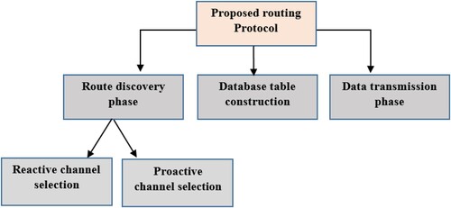
Generally, our routing protocol consists of three phases: (1) route discovery, which is also divided into two phases: route discovery with reactive channel selection and route discovery with proactive channel selection. (2) Data transmission to test our paths, and (3) Database table construction based on statistical results after observing the network transmission process for a time, as depicted in Figure 1.

Figure 1. Proposed routing protocol.

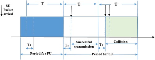
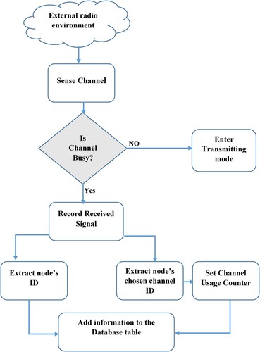
The network is assumed to contain a variety of PUs, each of which is capable of occupying a dedicated channel. We include time and simulate the existence of PUs into our procedures to make them more realistic. For analytical purposes, we adopt the representation of PU signals as numerous periods randomly clipped from each channel, as used in Darabkh et al. (2021). Any channel that has a PU or SU in it is deemed busy since only one user may be occupied by a channel at a time. Over and above that, the priority to use this channel is granted to the PUs, thus if an SU occupies the channel and the PU suddenly appears, the SU should stop transmitting and switch to another channel. Every cycle, where the duration of a cycle is identified by the PU's Tolerable Interference Delay (TID), each SU should keep an eye on the PU's actions to ascertain the availability of channels. Principally, the cycle is partitioned into a pair of parts, namely: sensing and transmission. The sensing time is governed by various factors, including the signal-to-noise ratio, the position of the SUs, and the detection possibility of the PUs. Consequently, the sensing time for one channel is different among SUs and is different for each channel. It is noteworthy that energy-based detection is adopted to see if the channel contains any users, and CSMA/CA is used as a MAC layer protocol. Figure 2 shows the channel utilization model in IEEE 802.22 standard.

Figure 2. Channel utilization model.

The positions of the SU nodes, the birth and death rates of SUs, the entire set of channels in the CRN, and the positions of PUs are all taken for granted. Additionally, the monitoring duration for each channel is arbitrarily chosen to range from one to one hundred milliseconds, with one second being assumed for TID. As indicated by $\mathrm{BW},$ however, it is believed that every channel has the same bandwidth. When the received SINR is compared with a predetermined threshold, the model that calculates the $\mathrm{BW}$ is taken into consideration. According to Salameh and El-Khatib (2019), if SINR exceeds a predefined threshold (${\mu }^{\ast }$) in this bandwidth model, the value of $\mathrm{BW}$ equals 1 bit per Hz per second. As a result, the bit rate (R) of the channel in bits per second is provided by the equation below (Salameh & El-Khatib, 2018): (1) $R=\{\begin{array}{cc}\mathrm{BW}& \mathrm{SINR}\ge {\mu }^{\ast },\\ 0& \mathrm{SINR}<{\mu }^{\ast }.\end{array}$(1) It is noteworthy that regarding the availability of channels, we consider and modify the two types of channels mentioned in the Cross-Layer Routing Protocol (CLRP) (Saifan et al., 2013) and in PDPS (Saifan et al., 2019), where they considered two types of channels: (i) a set of deterministically available channels assigned for each individual node (where nodes are responsible for sensing it periodically), (ii) and probabilistically available channels that were available with a certain probability (which represents the rest of the channels in the network).

Unlike PDPS (Saifan et al., 2019) and CLRP (Saifan et al., 2013) protocols, we take into account all channels in the network (deterministic and probabilistic channels) without assigning a specific set of channels to every node to avoid wasting time resulting from the periodic sensing process. Moreover, we take into consideration the probabilistically available channels to designate the activity of SUs in the network, as modified by Darabkh et al. (2021). Accordingly, we assume that all channels in the network should be sensed in the first sensing process to define the availability state for each channel. More, as evaluated by Liao et al. (2014) and Darabkh et al. (2019) for the Listen before Talk protocol (LBT), the sensing phase, which occurs before the network stabilizes, occupies one-third of the time slot.

Intrinsically, the idle probability, which reflects the channel availability of each channel, is determined after the first sensing as follows: (1) the available channel with idle probability = 1, which indicates no PU nor SU, (2) The busy channel with probability = 0, which indicates that the PU occupies this channel, and (3)The probabilistically available channel or unknown to be available channel as specified in Saifan et al. (2013, 2019) with an idle probability ranging from 0 to 1, which indicates the SU’s existence in the channel (Darabkh et al., 2021).

Impressively, the LBT concept lies at the heart of CSMA/CA that we use as a MAC layer protocol. Moreover, in JCARP, we consider all the channels in the pool and all paths formed using the previously mentioned types of channels (Darabkh et al., 2021). However, we use a list of channels for each node that consists of the available channels besides the probabilistically available just inside that node's range. Specifically, based on the distance between the channel and each SU. After that, before data transmission, each node performs a sensing procedure for the available channels and probabilistically available, accompanied by a frequent sensing procedure for the channel if selected to transmit through it.

The implementation of SUs’ activities in the network is by supposing two rates in a Poisson distribution, which are birth rate (β) and death rate (λ) (Saifan et al., 2019). To be more specific, the channel's probability of being either available or idle depends on the operations of the SUs (i.e. birth and death) as follows (Saifan et al., 2019).

In further detail, the channel has a probability of being idle or available based on the SUs’ operations (birth and death) as follows (Saifan et al., 2019): (2) $P_r(H_0)={\displaystyle \frac{\lambda }{\lambda +\beta }.}$(2) Accordingly, the probability of the channel being busy ($H_1$) is implemented using the following equation (Saifan et al., 2019): (3) $P_r(H_1)={\displaystyle \frac{\beta }{\beta +\lambda }.}$(3)

The average expected time for the channel to be idle, derived from the exponential distribution of the interval between SUs arrivals, equals (Saifan et al., 2019): (4) $E(C{h}_1)={\displaystyle \frac{1}{\beta }.}$(4) The Switching Time (SW), which means the time that SUs need to move to another channel to continue their transmission (if it is interrupted), is estimated as follows (Saifan et al., 2019): (5) $S{W}_{C{h}_1\mathrm{\&C}{h}_2}=\alpha |f_1-f_2|,$(5) where, α is the constant of a SW in seconds per Megahertz, and $f_1$, $f_2$ are the respective central frequencies of the two channels $C{h}_1\mathrm{\&}\mathrm{C}{h}_2$ (Darabkh et al., 2021; Saifan et al., 2019). The following equation is used to compute transmission time ($T_{T_x}$) (Darabkh et al., 2021; Saifan et al., 2019): (6) $T_{T_x}=\mathrm{TID}-\mathrm{ST}-\mathrm{SW}.$(6) The intermediate node that exists in several paths is assumed to have an initial load ($L_w$), which indicates the entire time necessary to serve all pathways, instead of the one desired Furthermore, the $L_w$ includes sensing channels in paths, transmitting and receiving over all paths. It is worth noting that the path desired is excluded from the initial load to calculate our delay time accurately (Darabkh et al., 2021). The following equation is used to compute the initial load ($L_w$) (Darabkh et al., 2021): (7) $L_w=S{T}_{P-1}-T{X}_{p-1},$(7) where, P is the number of paths, $S{T}_{P-1}$ denotes the sensing time for channels in other paths. On the other hand, $T{X}_{p-1}$ represents the receiving and sending time on other paths.

The throughput is represented by the transmission time per cycle to compute the maximum throughput achievable on the path to be discovered (Darabkh et al., 2021; Saifan et al., 2019). Thus, the throughput of a CR node w that receives data on channel $C{h}_1$ and sends data on channel $\mathrm{C}{h}_2$ is given by this equation (Darabkh et al., 2021; Saifan et al., 2019): (8) $T_{T_{xmax}}=\mathrm{TID}-L_w-S{T}_{C{h}_1}-S{T}_{C{h}_2}-\alpha |f_1-f_2|.$(8) The following equation is used to calculate the throughput in bits per second (Darabkh et al., 2021; Saifan et al., 2019): (9) $T{H}_{max}={\displaystyle \frac{T_{T_x}^{max}\times \mathrm{BW}}{\mathrm{HC}},}$(9) where $R=\mathrm{BW}$, as previously stated in Equation (1), and $\mathrm{HC}$ in JCARP is the path's hop count (Darabkh et al., 2021).

4. The proposed protocol

This section covers the following topics: reactive channel selection (forwarding RRQP), database table establishment, proactive channel selection (forwarding RRQP), reverse path, and data transmission.

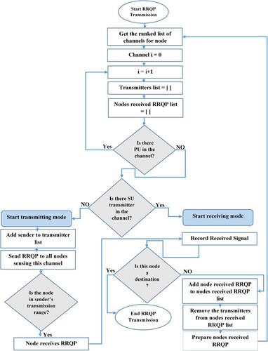
4.1. Reactive channel selection (Forwarding RRQP)

We have two modes in any route discovery (forwarding RRQP): (1) the transmitting mode, that belongs to the node needs to transmit a packet, therefore, it should sense the spectrum and select a channel for transmission. (2) The overhearing mode, that belongs to the node that can sense a channel and hear another node’s transmission. For more illustration, potential scenarios of the reactive channel selection are presented in Appendix 1.

Conspicuously, this can be explained as follows:

• Interestingly, in JCARP, we focus on building a network that operates in a fully distributed manner. Therefore, in order to accomplish our aim, we first eliminate the CCC and, rather than creating a neighbours’ database, propose a MAC layer technique based on the CSMA/CA protocol to address the spectrum sharing issue between SUs. Eliminating the neighbours’ table will also cut down on the quantity of control overhead messages sent out, as well as the time needed to locate neighbours in order to create and update the table.

• During the route discovery phase, each node searches for and finds every channel in its immediate vicinity. It then compiles a list of all the channels that are available or likely to become accessible within its transmission range. By doing this, we guarantee that we can preserve the viability and practicality of our assumption while designing many pathways (routes) by employing the majority of the network's channels. As a result, before any transmission starts, this sensing time is added.

• The PU-occupied channel is considered unavailable, whereas the SU-occupied channel is considered probabilistically accessible. This is an important distinction to make between the two detection processes in the sensing process. Energy-based detection is used to identify both SU and PU emitters simultaneously. Moreover, the leaky oscillator signals that emerge throughout the SU sensing procedure to separate SUs from PUs following energy-based detection provide the basis for the detection of SUs (Chaman et al., 2018; Cheng et al., 2017; Darabkh et al., 2021; Shao et al., 2020). Every leaking signal must thus have a unique ID. As mentioned earlier, that the idle channel is exclusively utilized, signifying the absence of both PUs and SUs within it.

• Prior to selecting a channel at random from this list of available channels, the source node prepares its associated list of channels in order to begin the transmitting mode operation. In addition, the source node creates a route request packet (RRQP) and appends extra data to it that connects the SU ID to the ID of the channel – a channel that is chosen at random to be sent over. Similarly, the source detects this channel, broadcasts RRQP over it, and all nodes that are within the source node's transmission range and have this channel added to their lists are eligible to receive the RRQP. The contents of the RRQP are listed in Table 1.

• The source node determines the downstream transmission time for all channels in its list, which facilitates the selection of another channel in case the source finds the first choice busy after sensing. Additionally, the downstream transmission time is calculated according to Equations (10) and (11), where the node computes this quality for a specified channel ($C{h}_1$), and the superscript (d) in the equation stands for downstream (Darabkh et al., 2021). Remarkably, if the channel is available, we use Equation (10) (Darabkh et al., 2021), and if it is probabilistically available; we use Equation (11) (Darabkh et al., 2021). (10) $T_{T_x}^d(C{h}_1)=\mathrm{TID}-L_w-S{T}_{C{h}_1}.$(10) (11) $T_{T_x}^d{}_{{}^{Pr}}(C{h}_1)=(\mathrm{TID}-L_w-S{T}_{C{h}_1})\times P_r(H_0).$(11)

• Every node receiving RRQPs is operating in overhearing mode. Therefore, in order to persist the RRQP forwarding, these intermediary nodes will create a message known as the basic message before producing their RRQPs (or local message). The optimum quality for each channel (best upstream quality) is contained in the basic message. Besides, the optimum throughput for every channel is calculated by comparing the received quality from the preceding intermediate node or the source node RRQP, which is called the item’s quality of channel i, with the estimated quality of the current node for the same channel, as presented in Equations (12) and (13) (Darabkh et al., 2021; Saifan et al., 2019).

• If we suppose that B is a node that receives the RRQP through the channel (1) from the source node A, then node B calculates the qualities of the basic message and subsequently the qualities of the local message based on the equations below. Specifically, if node B determines that channel (1) is available, then Equation (12) is used to calculate the basic message quality. On the other hand, if channel (1) is known as probabilistically available, then Equation (13) is used to compute the basic message quality where the basic message item b is multiplied by the idle probability. The basic message is denoted by the superscript (b) (Darabkh et al., 2021; Saifan et al., 2019). (12) $T_{T_x}^b(C{h}_1{)}_B=min\{q{(C{h}_1)}_A,T_{T_x}^d(C{h}_1)\}.$(12)

For probabilistically available channels (Darabkh et al., 2021; Saifan et al., 2019): (13) $T_{T_x}^b{}_{\mathrm{Pr}}(C{h}_1{)}_B=min\{q{(C{h}_1)}_A,T_{T_x}^d(C{h}_1)\}\times P_r(H_0),$(13) where, (14) $q(C{h}_1{)}_A=\left[\begin{array}{c}{T}_{T_x}^d{}_{\mathrm{Pr}}(C{h}_1{)}_A\mathrm{when}\mathrm{Ch}1\mathrm{is}\mathrm{probablistically}\mathrm{available}\\ T_{T_x}^d(C{h}_1{)}_A\mathrm{when}\mathrm{Ch}1\mathrm{is}\mathrm{available}\end{array}\right]$(14)

• After receiving the RRQP and formulating their basic message, the intermediary nodes switch to the transmitting mode to relay the RRQP, similar to the source node. Every intermediary node links the ID of the SU to the ID of the channel, adding further information to the RRQP like source.

• The fact that every node receiving RRQP from the source is concurrently attempting to convey its own RRQP is an intriguing point to note. In essence, multi-threading is used in our code, with the number of threads being equal to the number of nodes receiving the RRQP from the source node. This means that these nodes keep transmitting their RRQPs in the same way inside each corresponding thread.

• Substantially, the local message quality (or downstream) means finding the optimum upstream channel for each downstream channel. If the basic message item's channel is being investigated (i.e. i = 1), Equation (15) is employed to compute the temporary downstream quality (Darabkh et al., 2021; Saifan et al., 2019). (15) $Q_{\mathrm{down}}(C{h}_1{)}_B=min\{T_{T_x}^b{(C{h}_1)}_B,T_{T_x}^d{(C{h}_1)}_B\}.$(15)

• If the basic message item's channel is being studied and is verified to be probabilistically available; the downstream quality can be calculated using Equation (16) (Darabkh et al., 2021; Saifan et al., 2019): (16) $Q_{\mathrm{down}}^{\mathrm{Pr}}(C{h}_1{)}_B=\min \{T{{}_{T_x}^b}_{{}^{Pr}}{(C{h}_1)}_B,T_{T_x}^d{(C{h}_1)}_B\}.$(16)

If the channel under investigation is not the same as the basic message item's channel, the temporary downstream quality is provided in Equation (17) (Darabkh et al., 2021; Saifan et al., 2019): (17) $Q_{\mathrm{down}}(C{h}_1{)}_B=min\{T_{T_x}^b{(C{h}_i)}_B,T_{T_x}^d{(C{h}_1)}_B-S{T}_{C{h}_i\mathrm{at}B}-S{W}_{C{h}_1\mathrm{\&}C{h}_i}\},$(17) where $0\le i\le \mathrm{number}\mathrm{of}\mathrm{channel},\mathrm{and}i\ne 1$.

• The temporary downstream quality is given in Equation (18) if the channel under study is not the same as the basic message item's channel and is recognized to be probabilistically available (Darabkh et al., 2021; Saifan et al., 2019): (18) $Q_{\mathrm{down}}^{}{}^{\mathrm{Pr}}(C{h}_1{)}_B=\min \{T{{}_{T_x}^b}_{{}^{Pr}}{(C{h}_i)}_B,T_{T_x}^d{(C{h}_1)}_B-S{T}_{C{h}_i\mathrm{at}B}-S{W}_{\mathrm{Ch}{}_1\mathrm{\&}C{h}_i}\},$(18) where $0\le i\le \mathrm{number}\mathrm{of}\mathrm{channel},\mathrm{and}i\ne 1$

• The downstream quality (i.e. transmission time) is defined as the maximum of all temporary downstream qualities as follows (Darabkh et al., 2021; Saifan et al., 2019): (19) $Q_{\mathrm{down}}{}^{max}(C{h}_1)=max\{Q_{\mathrm{down}}(C{h}_1)\mathrm{from}\mathrm{all}\mathrm{temporary}\mathrm{qualities}\}.$(19)

• Eventually, the maximum value between the resulting downstream quality $Q_{\mathrm{down}}{}^{max}(C{h}_1)$ and the inaugural value of the item's downstream quality (which is −1) or another downstream quality if the node has already sent an RRQP before this time is the new message item in the RRQ, as given in Equation (20) (Darabkh et al., 2021; Saifan et al., 2019). Figure 3 illustrates the RRQP transmission process (Darabkh et al., 2021; Saifan et al., 2019). (20) $T_{T_x}^L(C{h}_1)=max\{Q_{\mathrm{down}}{}^{\max }{(C{h}_1)}_B,-1\}.$(20)

Figure 3. RRQP forwarding (reactive channel selection).

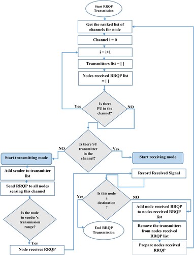
Table 1. The Format of RRQP.

Channel ID	NODE ID	Upstream Channel	Upstream Node	Downstream Quality	Mapping node’s selected channel ID with a node ID	Entity Length
The downstream Channel	This node ID	Previous Channel	Previous Node	The time for transmitting from the slot	One from downstream channels that are chosen for transmission with this node ID	In bits

4.2. Database table creation

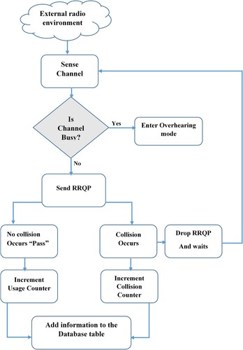
As nodes within a network might share idle spectrum, or accessible channels, within their communication range, competition between nodes to get access to these channels can arise. If spectrum sharing is not managed well, this competition can occasionally result in collisions. Furthermore, in order to ensure routing performance, choosing the optimal data transmission channel becomes essential. The CSMA/CA is utilized, as previously mentioned, to identify if a channel is busy or idle. Using the MAC layer protocol, posterior SUs attempt to access the spectrum during the route discovery phase, and this may occur concurrently. Two likely scenarios then arise. First, the SU successfully accesses the channel without encountering any other SUs (this is referred to in JCARP protocol as a ‘pass’ scenario). Last, in JCARP, a ‘collision’ occurs when an SU (or many SUs) attempt to access the same channel simultaneously as the SU trying to access it. This leads to data loss.

JCARP protocol works on the MAC layer to solve the channel sharing problem by building a database table in the long term for each SU as a reference to facilitate channel assignment and routing. Distinctly, studying the SUs’ behaviour in the transmission processes in the reactive channel selection. Precisely, in our code, we conduct our network many times (100 trials), which allows us to take the results of SUs choices in reactive channel selection over a specific number of experiments (e.g. 40 runs), and build a database table based on these results to produce a ranked list of channels. As a result, the ranked lists are used in the proactive channel selection phase to complete the rest of the trials (i.e. 60 experiments).

Essentially, we may take advantage of pass or collision scenarios that arise when SU is in the transmitting mode in order to construct our database table. Comparably, when the SU listens to the channel in the overhearing mode, it receives information from RRQPs. Using certain formulas, the obtained data from these two modes regarding the channels and the linked SU for these channels are inserted into the database table to provide statistics. As a result, we are able to categorize the channels based on the likelihood of their availability and provide a prioritized list of channels for every SU, which will be utilized during the proactive channel selection stage of the route discovery process. Notably, Appendix 2 includes an example that demonstrates the database table construction.

As mentioned before, while looking at the database table from the standpoint of the information source, it is separated into two sections: the transmitting and overhearing modes. Every SU has a database table, and every item in the table corresponds to a single channel from the SU's channel list. The database table attributes are shown in Table 2.

Table 2. Database table attributes.

	Transmitting mode		Receiving mode (listening to others)
Channel ID(M)	Usage counter	Collision counter	Node’s ID	Node’s Preferred (or chosen) channel	Channel’s usage counter	Channel’s Usage probability (%)	Channel’s Priority (ordering)

4.2.1. Database table information from the transmitting mode

From its list of accessible channels, the SU with an RRQP to transmit selects one channel randomly. When SU transmits RRQP via a channel, it indicates a successful transmission or a ‘pass’ scenario. Consequently, each time the SU successfully attempts to access the channel, the channel's utilization counter is incremented by one. However, as Figure 4 illustrates, collisions occur in this channel when several SUs select the same channel concurrently (from its list of accessible channels). Every time one of these SUs fails to access this channel, it causes its collision counter associated with it to increase by one. This process continues for all SUs involved in the aforementioned collisions (their RRQPs colliding in this channel). Depending on how often this channel is selected throughout trials, SU stores the prior data in the fields of the transmission mode in the database table for each channel.

Figure 4. SU in transmitting mode.

It is important to remember that in the event of a CSMA/CA collision, the packets from the SU that collide in this channel are discarded, and each node must wait a back off period before re-sensing the channel and sending data via it. JCARP drops the packets of several SUs that choose the same random channel at the same time. Our code employs multi-threading, thus each SU can access the channel at a different time. Based on this, we can conclude that we implement the back off time of JCARP (i.e. replicates the back off time essence).

4.2.2. Database table information from the overhearing mode

The CSMA/CA algorithm is utilized by the SU to detect the channel and determine if it is busy or idle. Interestingly, an RRQP may be received by this SU via this channel even if it discovers that another SU is using it, or if it is indeed busy. The SU now uses this RRQP to obtain the extra data included in the RRQP about other SUs and their channel preferences, such as the randomly chosen channel and SU's ID, as shown in Figure 5. Following that, the SU stores this data in the overhearing mode column for every channel in the RRQP including, node's ID along with node's selected channel columns. To precisely perform our mathematical calculations, however, the assumption is that every channel in SU's database table contains a channel usage counter, which is part of the data regarding other SU options. We fill this column in our code after completing certain computations, when SU increments the channel's usage counter by one or more based on how often this channel appears in other SU selections.

Figure 5. SU in overhearing mode.

4.2.3. Mathematical model of database table construction

Primarily, each SU in the database construction phase begins the statistics calculation for the list of all available channels for this SU. Thence, for each channel related to this SU, these statistics are divided into two parts:

4.2.3.1. Transmitting mode results

SU gets the Usage Counter ($\mathrm{UC}$) that represents the times that SU uses this channel successfully. Then, SU gets the Collision Counter ($\mathrm{CC}$) that represents the times that SU fails to access this channel.

In view of that, the summation result of these counters’ values is used to calculate the collision probability on this channel, as indicated by Equations (21) and (22). Remarkably, the Transmitting Mode is symbolized by a subscript ($\mathrm{TM}$). (21) $\mathrm{Total}\mathrm{usage}(C{h}_i{)}_{\mathrm{TM}}=\mathrm{UC}+\mathrm{CC}.$(21) (22) $\mathrm{Collision}\mathrm{Prob}(C{h}_i{)}_{\mathrm{TM}}=\mathrm{CC}/(\mathrm{Total}\mathrm{usage}).$(22)

4.2.3.2. Overhearing (or listening) mode results

SU calculates the Channel Repetition Counter$(\mathrm{CRC})$that represents the CRs in the choices of other SUs. Moreover, SU gets the Total number of Available Channels for this SU ($\mathrm{TAC}$).

We can calculate the percentage of CR ($\mathrm{Percentage}\mathrm{CR}$), which represents the CR in the choices of other SUs, over the total number of all available channels for this SU, as in Equation (23). Significantly, the Listening Mode is denoted by a subscript ($\mathrm{LM}$). (23) $\mathrm{Percentage}\mathrm{CR}(C{h}_i{)}_{\mathrm{LM}}=\mathrm{CRC}/\mathrm{TAC}.$(23) Ultimately, to calculate the Channel’s Usage Probability ($\mathrm{CUP}$), we should use an equation that incorporates the information about the channel from both modes, as given in Equation (24). In this equation, the percentage of channel usage is multiplied by the complement of the collision probability. As an outcome, each channel has a usage probability value, and the higher this value, the better this channel is for use. (24) $\mathrm{CUP}(C{h}_i)=(1-\mathrm{Percentage}\mathrm{CR})\times (1-\mathrm{Collision}\mathrm{Prob}).$(24) Extraordinarily, SU calculates the channel usage probability depending on the information and equations in the database table for each channel in the list of available channels, which belong to this SU. After that, these channels are ordered (in descending order) to form a new ranked list of available channels that facilitates channel selection in the proactive route discovery. Outstandingly, the order of the channels in the new ranked list determines the channel priority. The first channel in the ranked list is the channel with the highest priority to be used, and so on, until reaching the end of the list.

4.3. Proactive channel selection (forwarding RRQP)

The same process discussed in the reactive route discovery phase is applied in the proactive route discovery. But as you can see in Figure 6, SU selects one channel in this step from the prioritized list that comes from the examination of database tables. To be more specific, SU begins by determining if it is possible to send over the channel with the greatest priority. Furthermore, in the event that this channel is unavailable (e.g. PU is using it), SU attempts to access the next priority channel in the ranked list of channels, and further along.

Figure 6. RRQP forwarding (proactive channel selection).

Conversely, in our simulation code, in order to ensure that spectrum sharing is operating as intended, we assumed that in the event that the SU (receiver) chooses, if available, the next prioritized channel from the ranked list if it has received RRQP over the channel with the highest priority in its list (located at the top of the ranked list), and there are two SUs with the identical preferred channel. This process, essentially, helps prevent collisions among SUs.

4.4. Reverse path

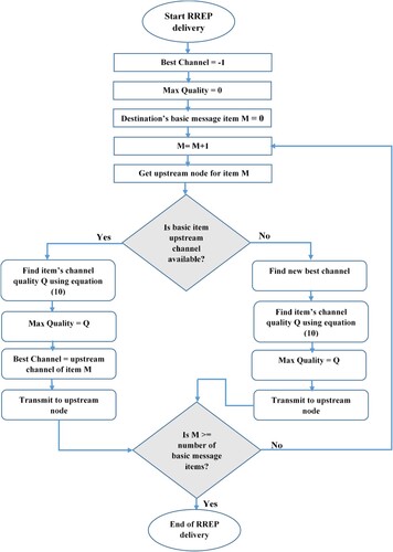
The process of creating and broadcasting a route reply packets (RREPs) may be summarized as follows:

• Our JCARP protocol starts by sending the route reply messages in the reverse path of the route discovery process, which follows both the proactive and reactive forwarding RRQP stages in route discovery.

• The destination node constructs its basic message, according to the optimum of the obtained RRQPs for each channel, after getting the RRQP from all upstream SUs. Additionally, the destination node generates an RREP containing the finest item (single item) from its basic message, which it then delivers, via the supreme upstream channels from a throughput standpoint, to all upstream nodes.

• The destination determines the quality of every available channel, as presented in Figure 7, using Equation (10) or Equation (8) if the reverse path's intermediate node assesses the quality of this channel (Darabkh et al., 2021; Saifan et al., 2019).

• It is worth remembering that the destination or intermediate transmits the RREP via the channel with the best quality, if it is available, in the reverse path. If this channel is busy, the destination or intermediate node (let's call it X) will endeavour to discover the subsequent optimum available channel between (X) and the next node that should receive RREP (let say Y).

• The node selects the greatest quality from $Q_1$ and $Q_2$, given a ‘prior channel’ from the previous hop. In particular, $Q_1$ related to node X (if X is the destination) is given using Equation (25) (Darabkh et al., 2021; Saifan et al., 2019), but if X is an intermediate node, then $Q_1$ is calculated using formula 26 (Darabkh et al., 2021; Saifan et al., 2019). (25) $Q_{1\mathrm{Destination}\mathrm{X}}=\mathrm{TID}-L_X-S{T}_{(C{h}_{i\mathrm{at}\mathrm{X}})},$(25) where $(0\le i\le \mathrm{number}\mathrm{of}\mathrm{channels})$. (26) $Q_{1\mathrm{Intermediate}\mathrm{node}\mathrm{X}}=\mathrm{TID}-L_X-S{T}_{(C{h}_i\mathrm{at}\mathrm{X})}-S{T}_{(\mathrm{previous}\mathrm{channel}\mathrm{at}\mathrm{Y})}-S{W}_{(C{h}_i\mathrm{\&}\mathrm{Previous}\mathrm{channel})},$(26) where $(0\le i\le \mathrm{number}\mathrm{of}\mathrm{channels})$.

• Prominently, Equation (26) shows that when the prior channel matches the channel in question i, node Y will observe channel i as well. Similarly, if the channel in question i is the same as the former best channel, node X will sense it as well, as shown in Equation (27) (Darabkh et al., 2021; Saifan et al., 2019). Notably, node X calculates $Q_1$to determine the quality of the channel in the reverse path. In contrast, Y calculates $Q_2$ for this channel in case of using it in the data transmission process (i.e. send a packet to X) (Darabkh et al., 2021; Saifan et al., 2019). (27) $Q_{2\mathrm{at}X}=\mathrm{TID}-L_Y-S{T}_{(C{h}_i\mathrm{at}\mathrm{Y})}-S{T}_{(\mathrm{old}\mathrm{best}\mathrm{channel}\mathrm{at}\mathrm{X})}-S{W}_{(C{h}_i\mathrm{\&}\mathrm{old}\mathrm{best}\mathrm{channel})},$(27) where $(0\le i\le \mathrm{number}\mathrm{of}\mathrm{channels})$.

• In actuality, the creation of the reverse pathways is dependent upon the multi-threading technique employed, in which succeeding nodes concurrently operate on many paths. Additionally, each node sends the RREP using the best available channel. As a result, the reverse route transmission is unicast, as RREPs are transmitted to specific nodes (upstream nodes) and most likely over the channels allocated in RRQP after they are verified to be available.

• The path with the highest throughput among all paths is identified by the source at the conclusion of the path discovery phase. Interestingly, the minimum throughput among all the hops in the path defines the throughput of the path.

Figure 7. RREP transmission at the destination.

4.5. Data transmission

Firstly, the source node depends on the path determined in the route discovery phase to transmit data over it. On each hop, each node monitors the recommended channel in the path and broadcasts a message to the next node using any other available channel if the recommended channel is not available. Amazingly, until the data reaches its destination, this operation will continue along the established path. However, because the time allocated for each transmission changes depending on the sensing time of the particular channel and the initial load of the nominated node, the size of the data packets can be altered.

5. Simulation results

In this section, the simulation results of our proposed protocol are presented, after conducting a comparison in the route discovery phase and data transmission phase with the PDPS protocol (Saifan et al., 2019), MC-HDRP, and MC-HDRP-CA routing protocols proposed in Darabkh et al. (2021). Also, this section includes detailed information about the simulation environment, the performance metric, and simulation parameters. Likewise, our results include route discovery and data transmission.

A Java-coded simulator was employed to perform the simulations. We utilize an Intel Core (TM) i5-7200U CPU running at 2.50 GHz with 8GB RAM in an HP Pavilion. Surprisingly, RRQP and RREP deliveries are forwarded through the threads. Table 3 schedules the baseline values of a few parameters. To test our findings, several settings were changed, though. In addition, every point in the figures denotes an average of 100 runs or trials.

Table 3. The simulation experiments’ parameters.

Parameter	Value
PU’s available number	12
SU’s available number in the network	50
Channels’ available number in the network	12
Channel bandwidth	6 MHz
Transmission range of PU node	500 ms
Transmission range of SU node	50 meters
Minimum and maximum monitoring time	1–100 ms
Minimum and maximum load	0.1–0.7 s
Network size of PUs	1000 × 1000 m^2
Source position of SU	At (0,0)
Destination position of SU	At (200,200)
Switching alpha: SW constant	1 ms per 1 MHz
SU nodes’ maximum transmission power	0.6 Watts
Tolerable interference delay of PU	1 s
Total number of trials	100

We consider throughput as a performance metric. It is possible to define throughput as the average number of successfully delivered packets per second. On the other hand, we determine the throughput by dividing the number of hops in the path by the multiplicity of the channel bandwidth and the transmission duration in each time slot. More precisely, since our simulations use the same channel bandwidth, the throughput is given in bits/sec/Hz without having to multiply by the bandwidth.

5.1. Simulation results and discussion

In our work, due to hybridization, the network sub sectioned into two parts: the reactive and the proactive channel selection in RRQP forwarding.

5.1.1. Our methodology’s results discussion

It is noteworthy that the nodes start working in the reactive phase to learn about the network and then build a database table that produces the ranked list of channels. Finally, the nodes enter the proactive phase. As we mentioned before, we conduct our network 100 runs (or trials), and each point of our graphs represents the average of 100 runs.

Accordingly, the 100 trials in our simulation are divided between those two parts. We examined different distributions of runs between reactive and proactive phases to find the optimal partition. In detail, for example, suppose that the SUs work in the reactive phase for 40 runs before switching to the proactive phase to continue the remaining 60 runs, as shown in the following Figure 8(a and b), Figure 9(a and b) and Figure 10(a and b), where we test different distribution of trials between the two phases and change some of the network's parameters to study the behaviour of our network.

Figure 8. Throughput vs. number of trials for reactive phase (experiment 1).

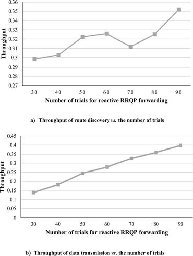
Figure 9. Throughput vs. number of trials for reactive phase (experiment 2).

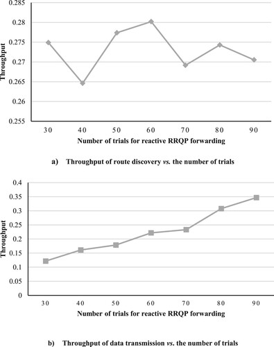
Figure 10. Reactive phase’s throughput vs. number of trials (experiment 3)

In Figure 8(a, b) or Experiment 1, we investigate the performance of our network under various numbers of trials regarding the reactive phase, where the number of SUs and channels are considered to be the default parameters in Table 3. Moreover, if we look at Figure 8, we will find that the optimal partition is to serve 90 trials in the reactive phase before switching to the proactive phase (i.e. the rest ten trials) because the network achieves the highest throughput at this point. That makes sense because when the nodes learn and build decisions after studying a long history, the resultant list of available channels for each node will be more accurate and stable. Therefore, there will be fewer unconnected nodes, and throughput will rise. On the other hand, the increase in throughput is more obvious in the data transmission, as shown in Figure 8(b), because it considers the optimum path (built in the route discovery phase) with changes in channels sometimes if required.

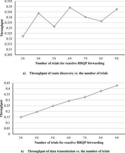
In Experiment 2, If we expand the number of channels to 40 channels for the same number of nodes (50 nodes), we notice results, as shown in Figure 9(a, b). Also, Figure 9(a) exhibits the behaviour of the network in route discovery, where the maximum throughput is attained when the number of trials dedicated to the reactive phase is 60 trials or 40 trials for the proactive part. Although it may appear that assigning a large number of trials to work in the reactive stage is not beneficial for the throughput, it is extremely significant for building the database table, and that is very clear in the data transmission phase, as viewed in Figure 9(b). Figure 9(b) indicates that increasing the number of channels allocated to the reactive phase increases throughput.

If we examine the influences of changing the number of channels on the throughput and behaviour of JCARP, we conclude that the increment of the number of channels has pros and cons. Firstly, increasing the number of channels may reduce throughput by increasing the number of hops in the route. Besides, the need to monitor the channels that form the path will increase to ensure the stability of the path. Additionally, building the database table depends on the number of collisions and the usage of channels. However, the increment in the number of channels proposes a variety of choices to each node, which mitigates the collision and the usage rates for each channel, leading to a relative deceleration in the operation of building the database table. The disadvantages of expanding the number of channels are outlined in the preceding paragraph.

Alternatively, one of the advantages of increasing the number of channels is to provide alternatives channels for nodes to be used if one channel becomes busy suddenly, which is more advantageous in the data transmission phase. More to the point, suppose that the increasing the number of channels may be exploited to build more routes in the route discovery phase rather than raising the number of hops in the paths, therefore this increment is beneficial for boosting the throughput. Ultimately, a trade-off is required to find the perfect number of channels, and usually, this is the point in the curve where the throughput stabilizes after appearing constant, which we shall explain in more detail in the next part.

In Figure 10 (a, b) or experiment 3, we increase the number of nodes to 60 for the default number of channels (i.e. 12 channels), and we observe the results. Interestingly, after observing Figure 10(a, b), we notice that we have the same behaviour as the previous experiment in both the route discovery phase and data transmission phase. Here too, the maximum throughput is achieved when the number of trials dedicated to the reactive phase is 60 runs (or 40 runs for the proactive part) in the route discovery phase. Further, in the data transmission phase, as illustrated in Figure 10(b), the curve of throughput vs. the number of trials related to the reactive phase is an ascending linear curve, implying that the throughput will rise as the number of runs assigned to the reactive phase increase.

If we study the effects of changing the number of nodes on the throughput and behaviour of our JCARP protocol, we conclude that the increment in the number of nodes has both pros and cons. Firstly, the increase in the number of nodes may decrease the throughput because the number of collisions may increase as nodes contend to access the available channels. The previous points represent drawbacks of increasing the number of nodes. However, one of the advantages of increasing the number of nodes is that it enlarges the number of nodes that can receive the RRQPs and then reduce the number of RRQPs forwarding stages, which means minimizing the number of hops as well as increasing throughput due to the increased number of paths.

Additionally, the construction of the database table depends on the number of collisions and channel usage, and in this scenario, the collision and usage rates will increase, thereby accelerating the operation of building the database table. In conclusion, a trade-off is needed to specify the best number of nodes, and usually, this is the point in the curve where the throughput after it seems constant, as we will discuss in the following subsection shortly.

5.1.2. Performance evaluation

This section appraises our JCARP protocol’s performance by comparing our results of the route discovery and data transmission phases throughputs with the results of MC-HDRP-CA, MC-HDRP, and PDPS protocols.

5.1.2.1. Route discovery phase

In this subsection, we conduct a comprehensive comparison between our results for route discovery phase throughput in [bits/sec/Hz] and the outcomes obtained from the MC-HDRP-CA, MC-HDRP, and PDPS protocols. We utilize the default parameters’ values as listed in Table 3 for all the subsequent experiments.

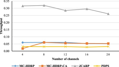
Through Figure 11, we noticed that our JCARP protocol outperforms other protocols because of the removing of the neighbour tables. Another reason is that nodes choose one channel exclusively to transmit over it in the discovery route (not all channels for all neighbours), which minimizes the interference between paths. In addition, nodes consider a list of available channels that indicate idle or in the range of these nodes (for probabilistically available channels), which allows these nodes to build probably steady and stable paths, thereby reducing the number of disconnected networks. In addition, we adopt multi-threading in forwarding RRQPs and RREPs, which increases the number of possible routes and improves the throughput. In general, if the number of channels grows, the throughput will rise as well. However, this increase in throughput will reach a settle point, where the throughput seems constant, which means the network reaches the optimal number of channels, as noticed in other protocols curves.

Figure 11. Throughput of route discovery vs. number of channels.

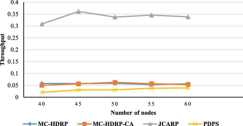
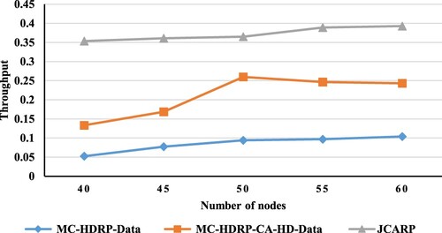
Figure 12 illustrates that the throughput rises with an increase in the number of nodes. This is attributed to the fact that as the number of nodes increases, connectivity also increases, resulting in enhanced throughput across all protocols. Nevertheless, the increase in throughput is limited by the escalating interference between nodes, which also intensifies with the increase in the number of nodes, which also explains why the curves seem to be constant because the increment in the connectivity is encountered by the increment of the interference. Secondly, as the number of nodes rises, the number of hops in each route increases, resulting in a reduction in throughput. Nonetheless, our JCARP protocol achieves the maximum throughput because with the growing number of nodes, there is a proportional increase in the number of nodes within the range capable of disseminating RRQPs, thereby expediting RRQP forwarding. Additionally, by distributing nodes across several paths, multi-threading guarantees that nodes are minimized in each path without compromising performance. Furthermore, adding more nodes is a great idea if you want to design a database table in which the number of collisions and channel usage grow as the nodes’ count rises whereas the number of channels stays the same. As a consequence, creating a database table proceeds more swiftly, resulting in a more precise list of channels for each node. This, in turn, diminishes the occurrence of disconnected networks and elevates throughput.

Figure 12. Throughput of route discovery vs. number of nodes.

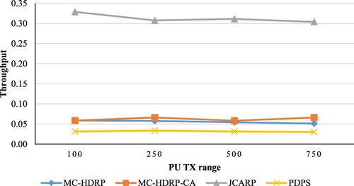
As depicted in Figure 13, with an increase in the PU transmission range, the number of available channels declines, leading to a reduction in throughput. Furthermore, the throughput is not sharply increased in the route discovery phase in all protocols because the nodes consider all channels in this phase, which provides more alternatives to deal with the increment in PUs transmission ranges. In our JCARP protocol, the impact of PUs transmission ranges on throughput is relatively obvious because the nodes have more constraints for using the channels. In other words, the nodes employ a channel list comprising either available channels (idle) or probabilistically available channels located within their range. Further, nodes consider the distance, which is calculated based on the transmission ranges of both SUs and PUs to determine if these channels are in the range of these nodes. In addition, this will appear in the data transmission phase, as we discuss shortly.

Figure 13. Throughput of route discovery vs. PU transmission range.

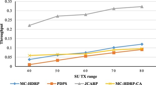
We may deduce from Figure 14 that the throughput will rise when the node (SUs)’s transmission range increases, specifically when the network size remains constant. In our JCARP protocol, increasing the nodes’ transmission ranges is very effective in light of the fact that the node's transmission range identifies the number of nodes that can receive RRQP. Moreover, the nodes that can receive RRQPs must be within the sender's transmission range, which implies that as the transmission range increases, the number of nodes that can hear this RRQP will increase too. Consequently, the number of nodes that will start the following RRQP forwarding stage will increase (nodes that received RRQP in the previous stage), which minimizes the number of RRQP forwarding stages needed (hops), leading to rising throughput.

Figure 14. Throughput of route discovery vs. SU transmission range.

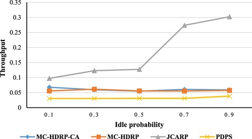
In order to investigate how changing idle probability impacts throughput, we should look at Figure 15. As depicted in this figure, the throughput seems constant in all protocols since they consider all channels in the route discovery phase regardless of the changes of idle probability. In contrast, the idle probability is a crucial factor in our work because – as we illustrated before – there are limitations on the channel to be used; one of these constraints is to use the available channel (i.e. idle no users in it). Specifically, if we raise the idle probability, we provide more channels for the nodes and vice versa. As a result, our JCARP protocol works better when the idle probability is high, precisely when the idle probability is 0.5 or more, as shown in Figure 15.

Figure 15. Throughput of route discovery vs. idle probability.

5.1.2.2. Data transmission phase

In this subsection, we compare our results of data transmission phase throughput [sec/n cycle time] with the results of MC-HDRP-CA and MC-HDRP protocols. To achieve high throughput, variable-length packets are employed. The number n represents the number of varying length packets essential to wrap up the message. We use the default parameters as listed in Table 3 for all the following experiments.

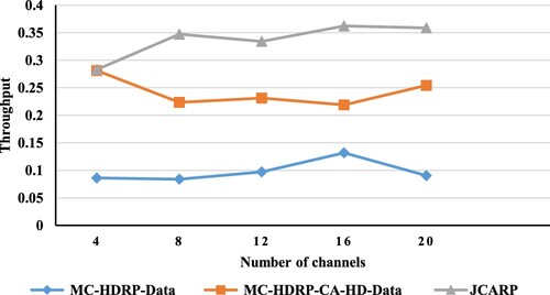
Figure 16 indicates that as the number of channels rises, data throughput improves, which makes sense since, during data transmission, the nodes rely on the best path that was created during the route discovery phase. Accordingly, if one of these best-path channels gets busy, the nodes must seek another available channel for this hop; hence increasing the number of channels is advantageous in reducing the number of disconnected networks and enhancing throughput.

Figure 16. Throughput of data transmission vs. number of channels

Figure 17 demonstrates that as the number of nodes rises, the throughput improves. As aforementioned, this is attributed to the fact that, increasing the number of nodes is helpful to establish multiple routes during the route discovery phase. As a result, that will reduce the number of disconnected networks, which means the best path most probably be stable, and data will be transmitted successfully. Additionally, using many nodes means many collisions and higher channel usage, subsequently, the database table is built rapidly, which also produces an accurate list of channels, making the choices of nodes more accurate. Eventually, the paths are more stable, and data transmission is done successfully.

Figure 17. Throughput of data transmission vs. number of nodes.

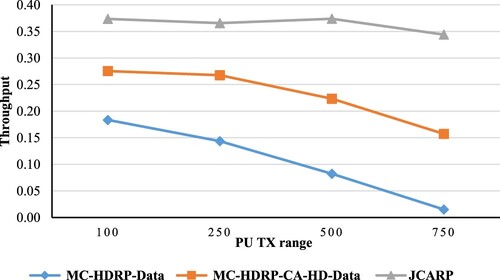
As demonstrated in Figure 18, an increase in PU's transmission range results in a reduction in throughput. This is because, as was previously mentioned during the route discovery phase, an increase in PU's transmission range mitigates the number of available channels, thereby causing the number of disconnected networks to rise and reducing throughput.

Figure 18. Throughput of data transmission vs. PU transmission range.

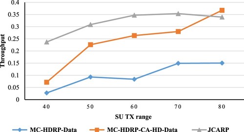
Similarly, as the route discovery phase behaviour, as the SU transmission range increase, the throughput will increase too. Owing to the fact that the nodes will have the ability to access more channels if required (i.e. if a channel in the path is busy), that is important to lessen the number of unconnected networks and improve the throughput, as seen in Figure 19.

Figure 19. Throughput of data transmission vs. SU transmission range.

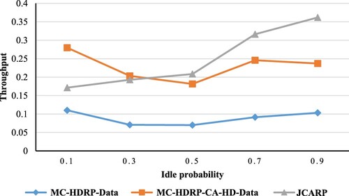
From Figure 20, we can conclude that as the idle probability increases, the throughput will rise. As seen in Figure 20, the HDRP-MC-CA achieves better throughput than our JCARP protocol in the lower idle probability, which is reasonable because we put restrictions to guarantee that nodes use the available channels only to make our work more practical. For illustration, if the idle probability declines, the number of available channels falls, and then the throughput declines, which affects our throughput value. However, other protocols are not affected by changes in idle probability because they use all channels without any limitations, which is impractical and leads to building non-stable paths.

Figure 20. Throughput of data transmission vs. idle probability.

6. Conclusions and future works

By creating a variety of applications, the IoT introduces a new way of living. IoT must include the capabilities of CRNs in order to avoid the bandwidth shortage. Although CRIoT received considerable attention, the work done in this area is still lacking compared to what is expected to be done. It is worth mentioning that CR provides effective spectrum-conscious communication approaches. Additionally, the adoption of CR technology in AHNs ensures that the spectrum is used efficiently to meet the growing burdens on wireless communications. Accordingly, because of spectrum scarcity, the number of spectrum holes is limited for SUs to communicate over them, which means the necessity for a perfect spectrum sharing protocol to organize the spectrum access between the contending SUs arises.

This research proposes a cooperative interaction between a hybrid routing protocol and a fully distributed spectrum management algorithm. In doing so, we introduce a CRAHN routing protocol, namely our JCARP protocol (i.e. no central entity), plus SUs cooperate without using a CCC or building neighbours tables, which present a practical and fully distributed network and minimize the control overhead. Precisely, our JCARP protocol minimizes the number of collisions in the channels and efficiently organizes spectrum sharing among SUs. It does so by considering routing transmission processes and channel history to adapt to modifications in the multichannel CRN environment. Besides, our JCARP protocol amalgamates the optimal traits of both reactive and proactive routing protocols, acting as a hybrid routing protocol. It achieves this by constructing a database table to facilitate the transition from the reactive routing protocol to the proactive routing protocol.

Interestingly, in constructing our database table for each node, we analyse the channel usage, whether it involves collisions or pass transmissions, during reactive channel selection trials throughout the route discovery phase. This process enables the establishment of a solid understanding of the list of channels associated with each node. Subsequently, the saved information in the database table over trials for each node is used for creating the ranked list of channels to start the proactive phase. Interestingly, using this database table and some imposed requirements on each node while forming their list of available channels is very helpful to building stable paths in our JCARP protocol, which minimizes the number of disconnected networks and increases the throughput. The simulation results indicate that our JCARP protocol performs better in terms of throughput than the MC-HDRP, MC-HDRP-CA, and PDPS protocols. It is worth pointing out that the cost of this significant improvement is having more storage for the database required for the proposed protocol to work efficiently in the hybrid mode.

For future directions, we can suggest some aspects to improve our design to be more comprehensive such as adding information about the PU's appearance in each channel to the database table, where the behaviour of PU should be studied to make parameters for PU's activities in our equation, which provides a more accurate decision about the channels. Moreover, paying more attention to PHY and MAC layers considerations, where the parameters that belong to these layers should be studied extensively in our JCARP protocol to design a more practical protocol. Additionally, Designing CRN includes the idea of mobility, as mobility is a crucial characteristic that accompanies wireless devices. Moreover, it is the main factor of network instability because mobile nodes detach from the network more frequently. Finally, examining other routing metrics rather than the throughput like the overhead, packet delivery ratio, and stability should be studied to prove JCARP's effectiveness.

Disclosure statement

No potential conflict of interest was reported by the author(s).

Additional information

Notes on contributors

Khalid A. Darabkh

Khalid A. Darabkh received the PhD degree in Computer Engineering from University of Alabama in Huntsville, USA, in 2007 with honors. He has joined the Computer Engineering Department at the University of Jordan as an Assistant Professor since 2007 and promoted exceptionally for professorship in 2016. He authored and co-authored of more than two hundred highly esteemed research articles. He is among World's Top 2% Scientists List, compiled by Stanford University in 2020, 2021, 2022, and 2023. He is the recipient of 2023 Distinguished Researcher Award for Scientific Schools at the University of Jordan. He is the recipient of 2020 Federation of Arab Scientific Research Councils Reward - Theme of Invention and Innovation. He is the recipient of 2016 Ali Mango Distinguished Researcher Award for Scientific Colleges and Research Centers in Jordan. He is further the recipient of the Most Cited Researchers Award at the University of Jordan at Scopus during 2017-2021.

Marwa H. Al-Tahaineh

Marwa H. AL-Tahaineh received MSc degree in Computer Engineering and Networks from the University of Jordan, Amman, Jordan, in 2022. Her research interests include cognitive radio networks and computer networks.

Andraws I. Swidan

Andraws I. Swidan is a professor at the Computer Engineering Department at the University of Jordan, Amman, Jordan and adjunct professor at McGill University, Montreal, Canada. Earned all his MSc and PhD degrees from Leningrad Electro-Technical Institute, Leningrad (Sant-Petesburg), Russia in 1979 and 1982, respectively. He has authored and co-authored tens of papers in international peer reviewed journals and attended several international conferences. His research interests include modular arithmetic and information security.

Appendices

Appendix 1: reactive channel selection illustration

As network protocols always consist of three components: the source which has datathat needs to be sent to a specific destination, and relay nodes in between that are responsible for transmitting the packets from source to destination and vice versa (path formation). The main concern in all routing protocols is how to find the best path for carrying data. Furthermore, this appendix presents several scenarios to show how JCARP works on the reactive channel selection (forwarding RRQP). Minutely, there are two possible scenarios based on studying the effects of selecting channels in reactive channel selection in route discovery route as follows:

No collisions occur between SUs (Best case)

In JCARP, each SU selects a random channel from its list of available channels to transmit RRQP over it. Subsequently, if the SUs choose different channels (i.e. no intersection between choices), as shown in Figure A1.

As depicted in the previous figure, each SU chooses one available channel randomly, where the green arrows represent the chosen situation with the number of this channel. For example, the source node selects $C{h}_5$ a channel to transmit on, and if we suppose that this channel is available in the lists of A and B nodes and they are positioned in the transmission range of the source node, then these nodes can receive the source's RRQP. Moreover, after receiving RRQP, nodes A and B forward their RRQPs simultaneously (multi-threading), thus A selects $C{h}_9$, and B selects $C{h}_3$, which means no collision occurs between their choices. After that, node A transmits RRQP over $C{h}_9$ as well node B transmits RRQP over $C{h}_3$. Consequently, nodes K and F have $C{h}_9$ in their lists, thus they receive this A's RRQP, and nodes K and G have $C{h}_3$ in their lists, and thus they can receive B's RRQP and so on till reaching the destination.

Collisions occur partially in some of SUs choices (Moderate case)

In this case, even though the collisions occur in some of Sus’ choices (i.e. two or more SUs select the same channel), there is still at least one way or (path) for RRQP to reach the destination, as seen in Figure A2. As depicted in Figure A2, the red arrows represent the collision situation accompanied by the channel's number, and the green ones represent the pass situation. No collisions occur in the choices of the following nodes: source, A, B, K, F, Z, and H, therefore we focus on the cases where the collisions occur; for example, the nodes G and k select $C{h}_2$ simultaneously, which leads to collision occurrence. As well, nodes N and X select the same channel, and the collision occur. As a result, the RRQPs don't reach nodes C, H, and S from the nodes that experienced collisions in their choices. Fortunately, nodes S and H receive the RRQP from other nodes, from nodes Z and X, respectively, as illustrated in our example. It is noteworthy that in our work, after detecting these collisions, the related packets are dropped then the nodes access these channels at different times.

It is noteworthy to mention that the worst case happens when the source chooses a channel that another source chooses simultaneously, and the collision occurs, as presented in Figure A3. However, this case doesn't appear in JCARP because our network includes only one source and one destination.

Appendix 2: database table construction and discussion

In this appendix, we propose an example of database table building in JCARP. Initially, to build the database table, each node studies the behaviour of transmission processes among several trials and saves information in this table. Further, the nodes make statistical operations to rank their list of available channels. If we assume that node A has a list of ten available channels, also node A collects information about these channels’ usage from the received RRQP in the reactive channel selection in forwarding RRQP phases, plus its history of using these channels, as shown in Table A1. Bearing in mind that we display a sample of nodes IDs and their selected channel, but these channels can be selected more than one time, and the repetition of these channels can be calculated from RRQPs, after finishing the reactive forwarding RRQP stage, as given in Table A2.

Table A1. Database table of node A.

	Transmitting mode		Receiving mode (listening to others)
Channel ID (M)	Usage Counter $(\mathrm{UC})$	Collision Counter $(\mathrm{CC})$	Node’s id	Node’s Preferred (or chosen) channel	Channel Repetition Counter $(\mathrm{CRC})$	Channel’s usage probability	Channel’s Priority (ordering)
Ch1	3	2	D	1
Ch3	2	5	Z	3
Ch5	5	3	C	5
Ch8	4	6	B	8
Ch10	2	2	I	10
Ch2	6	1	K	2
Ch9	4	4	E	9
Ch4	1	7	F	4
Ch12	9	2	H	12

Total number of available channels for this node ($\mathrm{TAC}$) = 9.

Table A2. A’s database table after calculating CUC.

	Transmitting mode		Receiving mode (listening to others)
Channel ID (M)	Usage Counter $(\mathrm{UC})$	Collision Counter $(\mathrm{CC})$	Node’s id	Node’s Preferred (or chosen) channel	Channel Repetition Counter $(\mathrm{CRC})$	Channel’s usage probability	Channel’s Priority (ordering)
Ch1	3	2	D	1	2
Ch3	2	5	Z	3	5
Ch5	5	3	C	5	3
Ch8	4	6	B	8	6
Ch10	2	2	I	10	2
Ch2	6	1	K	2	1
Ch9	4	4	E	9	4
Ch4	1	7	F	4	7
Ch12	9	2	H	12	2

Total number of available channels for this node ($\mathrm{TAC}$) = 9.

Firstly, we calculate the transmitting mode results for channel (1) as an example, based on Equations (21) and (22) as follows: $\mathrm{Total}\mathrm{usage}(C{h}_1{)}_{\mathrm{TM}}=2+3=5$ $\mathrm{Collision}\mathrm{Prob}(C{h}_1{)}_{\mathrm{TM}}=2/5=0.4$

Next, we calculate the overhearing mode results by determining the list of available channels size ($\mathrm{TAC}$) and using Equation (23) as follows: $\mathrm{Percentage}\mathrm{CR}(C{h}_1{)}_{\mathrm{LM}}=2/9=0.22$As a result, the channel’s usage probability is calculated based on Equation (24): $\mathrm{CUP}(C{h}_1)=(1-0.22)\times (1-0.4)=0.78\times 0.6=0.468$

Similarly, the previous procedure will be repeated for all channels that belong to node A, as seen in Table A3.

Eventually, after ranking the list of available channels in descending order. Subsequently, node A gets a new ranked list of available channels as follows: {Ch₂, Ch₁₂, Ch₁, Ch₅, Ch₁₀, Ch₉, Ch₈, Ch₃, Ch₄}.

Consequently, the new ranked list will be used in the proactive channel selection in forwarding RRQP, where the order of this list determines the priority of using this channel that means the ch12 has the highest priority, and so on. Moreover, the priority of channels appears in Table A4.

Figure A1. Reactive channel selection best case (no collisions).

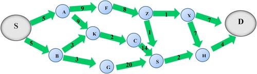
Figure A2. Route discovery moderate case (partial collision).

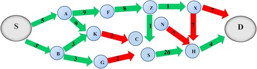
Figure A3. Route discovery worst case.

Table A3. A’s database table after calculating channel usage probability.

	Transmitting mode		Receiving mode (listening to others)
Channel ID (M)	Usage Counter $(\mathrm{UC})$	Collision Counter $(\mathrm{CC})$	Node’s id	Node’s Preferred (or chosen) channel	Channel Repetition Counter $(\mathrm{CRC})$	Channel’s usage probability	Channel’s Priority (ordering)
Ch1	3	2	D	1	2	0.468
Ch3	2	5	Z	3	5	0.127
Ch5	5	3	C	5	3	0.416
Ch8	4	6	B	8	6	0.133
Ch10	2	2	I	10	2	0.389
Ch2	6	1	K	2	1	0.762
Ch9	4	4	E	9	4	0.278
Ch4	1	7	F	4	7	0.027
Ch12	9	2	H	12	2	0.636

Total number of available channels for this node ($\mathrm{TAC}$) =  9.

Table A4. Final database table of node A.

	Transmitting mode		Receiving mode (listening to others)
Channel ID (M)	Usage Counter $(\mathrm{UC})$S	Collision counter $(\mathrm{CC})$	Node’s id	Node’s Preferred (or chosen) channel	Channel Repetition Counter $(\mathrm{CRC})$	Channel’s usage probability (%)	Channel’s Priority (ordering)
Ch1	3	2	D	1	2	0.468	3
Ch3	2	5	Z	3	6	0.127	8
Ch5	5	3	C	5	4	0.416	4
Ch8	4	6	B	8	7	0.133	8
Ch10	2	2	I	10	4	0.389	5
Ch2	6	1	K	2	3	0.762	1
Ch9	4	3	E	9	5	0.278	6
Ch4	1	7	F	4	8	0.027	9
Ch12	7	1	H	12	1	0.636	2

Total number of available channels for this node ($\mathrm{TAC}$) = 9.

References

- Alqahtani, A. S., Changalasetty, S. B., Parthasarathy, P., Thota, L. S., & Mubarakali, A. (2023). Effective spectrum sensing using cognitive radios in 5G and wireless body area networks. Computers and Electrical Engineering, 105, Article 108493. https://doi.org/10.1016/j.compeleceng.2022.108493
- Al-Rokabi, A., & Politis, C. (2014, June). SOAP: A cognitive hybrid routing protocol for mobile ad-hoc networks. In 2014 9th International Conference on Cognitive Radio Oriented Wireless Networks and Communications (CROWNCOM), IEEE (pp. 353–359). Oulu, Finland.
- Bany Salameh, H., Al-Nusair, N., Alnabelsi, S. H., & Darabkh, K. A. (2020). Channel assignment mechanism for cognitive radio network with rate adaptation and guard band awareness: Batching perspective. Wireless Networks, 26(6), 4477–4489. https://doi.org/10.1007/s11276-020-02344-w
- Bany Salameh, H., Derbas, R., Aloqaily, M., & Boukerche, A. (2019, November). Secure routing in multi-hop iot-based cognitive radio networks under jamming attacks. In Proceedings of the 22nd International ACM Conference on Modeling, Analysis and Simulation Of Wireless and Mobile Systems (pp. 323–327). New York, NY, USA.
- Chaman, A., Wang, J., Sun, J., Hassanieh, H., & Choudhury, R. R. (2018, November). Ghostbuster: Detecting the presence of hidden eavesdroppers. In Proceedings of the Annual International Conference on Mobile Computing and Networking, MOBICOM. New Delhi, India.
- Che-aron, Z., Abdalla, A. H., Hassan, W. H., Abdullah, K., & Rahman, M. A. (2014, November). E-D2CARP: A joint path and spectrum diversity-based routing protocol with an optimized path selection for cognitive radio ad hoc networks. In 2014 IEEE 2nd International Symposium on Telecommunication Technologies (ISTT) (pp. 39–44). Langkawi, Malaysia.
- Cheng, W., Zhang, X., & Zhang, H. (2017, May). Pilot-based full-duplex spectrum-sensing and multichannel-MAC over non-time-slotted cognitive radio networks. In IEEE INFOCOM 2017-IEEE Conference on Computer Communications (pp. 1–9). Atlanta, GA, USA.
- Darabkh, K. A., Al-Khazaleh, H. F., Al-Zubi, R. T., Alnabelsi, S. H., & Salameh, H. B. (2023). Efficient routing protocol for optimal route selection in cognitive radio networks over IoT environment. Wireless Personal Communications, 129(1), 209–253. https://doi.org/10.1007/s11277-022-10093-6
- Darabkh, K. A., Al-Tahaineh, M. H., Swidan, A. I., & Salameh, H. B. (2022, December). A novel routing protocol for software defined radios. In 2022 Ninth International Conference on Software Defined Systems (SDS) (pp. 1–5), Paris, France.
- Darabkh, K. A., Amro, O. M., Al-Zubi, R. T., & Salameh, H. B. (2021). Yet efficient routing protocols for half-and full-duplex cognitive radio Ad-Hoc networks over IoT environment. Journal of Network and Computer Applications, 173, Article 102836. https://doi.org/10.1016/j.jnca.2020.102836
- Darabkh, K. A., Amro, O. M., Salameh, H. B., & Al-Zubi, R. T. (2019). A–Z overview of the in-band full-duplex cognitive radio networks. Computer Communications, 145, 66–95. https://doi.org/10.1016/j.comcom.2019.06.007
- Darabkh, K. A., Awawdeh, B. R., Saifan, R. R., Khalifeh, A. F., Alnabelsi, S. H, & Bany Salameh, H. (2022, December). An Efficient Routing Protocol for Full-Duplex Software Defined Radios,” In Proceedings of the Ninth International Conference on Software Defined Systems (SDS2022), Paris, France.
- Darabkh, K. A., Awawdeh, B. R., Saifan, R. R., Khalifeh, A. F., Alnabelsi, S. H., & Bany Salameh, H. (2023). Routing in cognitive radio networks using adaptive full-duplex communications over IoT environment. Wireless Networks, 29(3), 1439–1463. https://doi.org/10.1007/s11276-022-03210-7
- Darabkh, K. A., Khazaleh, H. F, Al-Zubi, R. T., Alnabelsi, S. H., & Bany Salameh, H. (2022, November, December). An improved and stable routing algorithm for cognitive radio based IoT networks. In Proceedings of The 9th International Conference on Internet of Things: Systems, Management and Security (IOTSMS 2022), Milan, Italy.
- Ding, L., Melodia, T., Batalama, S., & Medley, M. J. (2009, October). Rosa: Distributed joint routing and dynamic spectrum allocation in cognitive radio ad hoc networks. In Proceedings of the 12th ACM International Conference on Modeling, Analysis and Simulation of Wireless and Mobile Systems (pp. 13–20). Tenerife, Canary Islands, Spain.
- Dutta, N., & Sarma, H. K. D. (2023). Primary user supported routing protocol for cognitive radio ad hoc networks in search of higher throughput. International Journal of Communication Systems, 36 (11), Article e5511. https://doi.org/10.1002/dac.5511
- Elrhareg, H., Ridouani, M., & Hayar, A. (2019, October). Routing protocols on cognitive radio networks: Survey. In 2019 IEEE International Smart Cities Conference (ISC2) (pp. 296–302). Casablanca, Morocco.
- Fernando, X., & Lăzăroiu, G. (2023). Spectrum sensing, clustering algorithms, and energy-harvesting technology for cognitive-radio-based internet-of-things networks. Sensors, 23(18), Article 7792. https://doi.org/10.3390/s23187792
- Foukalas, F., Karetsos, G. T., & Chatzimisios, P. (2013, August). Cross-layer design of csma/ca with spectrum sensing for cognitive radio networks. In ISWCS 2013: The Tenth International Symposium on Wireless Communication Systems (pp. 1–5). Ilmenau, Germany.
- Han, X., & Schormans, J. (2016). Cross-layer queueing analysis for aggregated ON–OFF arrivals with adaptive modulation and coding. IET Communications, 10(17), 2336–2343. https://doi.org/10.1049/iet-com.2015.0704
- Hu, F., Chen, B., & Zhu, K. (2018). Full spectrum sharing in cognitive radio networks toward 5G: A survey. IEEE Access, 6, 15754–15776. https://doi.org/10.1109/ACCESS.2018.2802450
- Jia, J., Wang, X., & Chen, J. (2015). A genetic approach on cross-layer optimization for cognitive radio wireless mesh network under SINR model. Ad Hoc Networks, 27, 57–67. https://doi.org/10.1016/j.adhoc.2014.11.020
- Khasawneh, M., Azab, A., Alrabaee, S., Sakkal, H., & Bakhit, H. (2023). Convergence of IoT and cognitive radio networks: A survey of applications, techniques, and challenges. IEEE Access, 11, 71097–71112. http://doi.org/10.1109/ACCESS.2023.3294091
- Khurana, S., & Upadhyaya, S. 2019. Classification of routing protocols based on routing metrics in cognitive radio AD HOC networks. International Journal of Recent Technology and Engineering (IJRTE), 8(3), 8815–8826.
- Li, F., Lam, K. Y., Li, X., Sheng, Z., Hua, J., & Wang, L. (2020). Advances and emerging challenges in cognitive internet-of-things. IEEE Transactions on Industrial Informatics, 16(8), 5489–5496. https://doi.org/10.1109/TII.2019.2953246
- Liao, Y., Wang, T., Song, L., & Han, Z. (2014, December). Listen-and-talk: Full-duplex cognitive radio networks. In 2014 IEEE Global Communications Conference (pp. 3068–3073). Austin, TX, USA.
- Lo, B. F. (2011). A survey of common control channel design in cognitive radio networks. Physical Communication, 4(1), 26–39. https://doi.org/10.1016/j.phycom.2010.12.004
- Malik, T. S., Malik, K. R., Sanaullah, M., Hasan, M. H., & Aziz, N. (2022). Non-cooperative learning based routing for 6G-IoT cognitive radio network. Intelligent Automation & Soft Computing, 33(2), 809–824. https://doi.org/10.32604/iasc.2022.021128
- Musa, A., Bany Salameh, H., Abu Sannad, N., Halloush, R., & Darabkh, K. (2020). Spectrum management with simultaneous power-controlled assignment decisions in cognitive radio networks. Concurrency and Computation: Practice and Experience, 32(21), Article e5224. https://doi.org/10.1002/cpe.5224
- Muzaffar, M. U., & Sharqi, R. (2024). A review of spectrum sensing in modern cognitive radio networks. Telecommunication Systems, 85 (2), 347–363. https://doi.org/10.1007/s11235-023-01079-1
- Nayyar, A. (2018, December). Comprehensive analysis of routing protocols for cognitive radio Ad-hoc networks (CRAHNs). In 2018 International Conference on Intelligent and Innovative Computing Applications (ICONIC), pp. 1–7, Mon Tresor, Mauritius.
- Pourpeighambar, B., Dehghan, M., & Sabaei, M. (2019). Joint routing and channel assignment using online learning in cognitive radio networks. Wireless Networks, 25(5), 2407–2421. https://doi.org/10.1007/s11276-018-1672-9
- Raj, R. N., Nayak, A., & Kumar, M. S. (2020). Spectrum-aware cross-layered routing protocol for cognitive radio ad hoc networks. Computer Communications, 164, 249–260. https://doi.org/10.1016/j.comcom.2020.10.011
- Rodriguez-Colina, E., Ramos-R, V. M., & Laguna-Sanchez, G. (2012, May). Cross layer analysis for a dynamic spectrum allocation system. In 2012 Workshop on Engineering Applications (pp. 1–6).
- Roy, S. S., & Zade, P. L. (2018). Performance optimization of ad hoc on demand vector routing protocol in cognitive radio network. I.J. Wireless and Microwave Technologies, 8(3), 23–32.
- Saifan, R., Kamal, A. E., & Guan, Y. (2013, December). A cross-layer routing protocol (CLRP) for cognitive radio network. In 2013 IEEE Global Communications Conference (GLOBECOM) (pp. 896–901). Atlanta, GA, USA.
- Saifan, R., Msaeed, A. M., & Darabkh, K. A. (2019). Probabilistic and deterministic path selection in cognitive radio network. IET Communications, 13(17), 2767–2777. https://doi.org/10.1049/iet-com.2019.0748
- Salameh, H. A. B., & El-Khatib, R. (2019). Spectrum-aware routing in full-duplex cognitive radio networks: An optimization framework. IEEE Systems Journal, 13(1), 183–191. https://doi.org/10.1109/JSYST.2018.2810207
- Salih, Q. M., Rahman, M. A., Al-Turjman, F., & Azmi, Z. R. M. (2020). Smart routing management framework exploiting dynamic data resources of cross-layer design and machine learning approaches for mobile cognitive radio networks: A survey. IEEE Access, 8, 67835–67867. https://doi.org/10.1109/ACCESS.2020.2986369
- Salih, Q. M., Rahman, M. A., Asyhari, A. T., Naeem, M. K., Patwary, M., Alturki, R., & Ikram, M. A. (2023). Dynamic channel estimation-aware routing protocol in mobile cognitive radio networks for smart IIoT applications. Digital Communications and Networks, 9(2), 367–382. https://doi.org/10.1016/j.dcan.2023.01.019
- Senthamizh, S., & Gopinath, P. G. (2015). Cross layer design for minimizing the delay in cognitive radio based WMNs. International Journal of Innovative Science Engineering and Technology, 4(6), 449–453.
- Shao, C., Jang, W., Park, H., Sung, J., Jung, Y., & Lee, W. (2020). Phantom eavesdropping with whitened RF leakage. IEEE Wireless Communications Letters, 9(2), 232–235. https://doi.org/10.1109/LWC.2019.2949316
- Singh, K., & Moh, S. (2016). Routing protocols in cognitive radio ad hoc networks: A comprehensive review. Journal of Network and Computer Applications, 72, 28–37. https://doi.org/10.1016/j.jnca.2016.07.006
- Singhal, C., & Rajesh, A. (2020). Review on cross-layer design for cognitive ad-hoc and sensor network. IET Communications, 14(6), 897–909. https://doi.org/10.1049/iet-com.2019.0636
- Singhal, D., & Garimella, R. M. (2015). Cognitive cross-layer multipath probabilistic routing for cognitive networks. Wireless Networks, 21(4), 1181–1192. https://doi.org/10.1007/s11276-014-0847-2
- Teekaraman, Y., Manoharan, H., Basha, A. R., & Manoharan, A. (2023). Hybrid optimization algorithms for resource allocation in heterogeneous cognitive radio networks. Neural Processing Letters, 55(4), 3813–3826. https://doi.org/10.1007/s11063-020-10255-2
- Teng, Y., & Song, M. (2017). Cross-layer optimization and protocol analysis for cognitive ad hoc communications. IEEE Access, 5, 18692–18706. https://doi.org/10.1109/ACCESS.2017.2671882
- Yarnagula, H. K., Deka, S. K., & Sarma, N. (2017). A cross-layer based location-aware forwarding using distributed TDMA MAC for ad-hoc cognitive radio networks. Wireless Personal Communications, 95(4), 4517–4534. https://doi.org/10.1007/s11277-017-4098-2
- Zareei, M., Islam, A. M., Mansoor, N., Baharun, S., Mohamed, E. M., & Sampei, S. (2016). CMCS: A cross-layer mobility-aware MAC protocol for cognitive radio sensor networks. EURASIP Journal on Wireless Communications and Networking, 2016(1), 1–15. https://doi.org/10.1186/s13638-016-0652-y
- Zheng, K., Wang, J., Liu, X., Yao, X.-W., Xu, Y., & Liu, J. (2023). A hybrid communication scheme for throughput maximization in backscatter-aided energy harvesting cognitive radio networks. IEEE Internet of Things Journal, 10(18), 16194–16208. https://doi.org/10.1109/JIOT.2023.3267453