Properties of k-record posteriors for the Weibull model

Abstract

Bayesian inference is one of the most important issues under the model selection procedures in statistics. This paper performed a Bayesian analysis of posteriors using a well-known Weibull model with high fitting performance. We proved that there exist necessary and sufficient conditions for the priors to yield proper posteriors and finite posterior moments based on record data. Moreover, we found a significant implication through different well-known objective priors. Finally, for illustration purposes, a Monte Carlo simulation procedure is done in the paper. The results indicate that the developed inference may have a significant contribution within Bayesian analysis through applications across different areas.

Keywords:

• Weibull distribution
• objective prior
• proper posterior
• moments
• records

MSCs (2010):

• 62F15
• 62N05

1. Introduction

Record values are seen as observations that overpass the previous ones in a sequence of lifetime observations. They were introduced in Chandler (1952) as a framework that deals with the time of occurrence of weather extremes from a sequence of weather conditions which can be interpreted as realizations of independent and identically distributed (iid) random variables. It has been acknowledged that records have a major overall value in sports, economics, meteorology, medicine and so on.

Record values occupy a special place in the insurance market. Their use has had outstanding impact on overall insurance market development throughout history. Insurance claims are the best example of impact that record values have in the insurance market, especially in insurance claims where portfolio strongly depends on the occurrence of record events in e.g. earthquakes or weather disasters (Balakrishnan et al., 1996). In addition, record values have a major impact on basic daily activities such as recording athletic achievements and predicting future ones (Empacher et al., 2023; Gembris et al., 2007). Such record events are obtained sequentally, directly recorded by appropriate measure instruments or by some other intuitive methods. Other examples may be found in breaking wooden beams (Glick, 1978), extreme weather conditions (Benestad, 2003), biology (Kauffman & Levin, 1987), etc. Interested readers may refer to Arnold et al. (2011), Nevzorov (2000) and Wergen (2013) for a detailed review of recent developments within this theory.

In this paper, we study the so-called kth record values. They were introduced in Dziubdziela and Kopociński (1976) from which we have the following definition of upper kth record values and upper kth record times. Let $T_{1,k}=k,R_{1\left(k\right)}=X_{1:k}$ and for $n\ge 2$, let $T_{n,k}=min\{j:j>T_{n-1,k},X_j>X_{T_{n-1,k}-k+1:T_{n-1,k}}\}$, where $X_{i:m}$ denotes the ith order statistics in a sample of size m from the underlying iid sequence $\{X_i,i\ge 1\}$. Then, the sequence $\{T_{n,k},k\ge 1\}$ is denoted as a sequence of kth upper record times while the sequence $\{R_{n\left(k\right)}=X_{T_{n-1,k}-k+1:T_{n-1,k}},n\ge 1\}$ is denoted as a sequence of upper kth record values.

To add additional input, let us generate a sample of 30 random observations from a standard exponential distribution for presenting a step-by-step extraction guidance on the upper kth records. The observations are 0.7423, 0.6271, 1.0574, 0.3278, 0.3473, 1.6076, 1.0107, 0.3315, 0.1660, 0.6252, 0.1356, 0.1816, 0.3203, 0.2604, 0.4287, 0.2552, 0.2088, 0.0815, 0.3717 and 0.2175. Let us take k=2. The first upper second record time ($T_{1,2}$) and value ($R_{1\left(2\right)}$) are obtained as $\begin{array}{r}{T}_{1,2}=2,R_{1\left(2\right)}=X_{1:2}=min\{X_1,X_2\}=\mathrm{0.6271.}\end{array}$For n=2, we have $\begin{array}{r}{T}_{2,2}=min\{j:j>2,X_j>X_{1:2}\}=3,R_{2\left(2\right)}=X_{2:3}=\mathrm{0.7423.}\end{array}$Next, for n=3, we have $\begin{array}{r}{T}_{3,2}=min\{j:j>3,X_j>X_{2:3}\}=4,R_{3\left(2\right)}=X_{3:4}=\mathrm{1.0574.}\end{array}$Based on the sample, there will be no more upper second records, so the extracted second upper records are 0.6271, 0.7423 and 1.0574.

Basically, an upper kth record value is the kth largest yet seen in a partial sample. For the case k=1, kth records reduce to ordinary records. From the above sample, we have extracted ordinary records as follows: 0.7423, 1.0574 and 1.6076.

Record statistics have found their place in various statistical fields such as characterization problems (Juhás & Skřivánková, 2014; Vidović, 2021), goodness of fit tests (Doostparast, 2011), predictions (Volovskiy & Kamps, 2023; Wang & Ye, 2015), information theory (Syam & Barakat, 2022), reliability analysis (Kizilaslan & Nadar, 2017), etc.

Let $R_{1\left(k\right)},R_{2\left(k\right)},\dots ,R_{n\left(k\right)}$ be the first n upper kth records from the Weibull distribution with probability density function (pdf) and cumulative density function (cdf) (1) $\begin{array}{r}f(x|\mu ,\text{β})=\text{β}{\mu }^{\text{β}}{x}^{\text{β}-1}{\mathrm{e}}^{-{\mu }^{\text{β}}{x}^{\text{β}}},x>0,\end{array}$(1) and (2) $\begin{array}{r}F(x|\mu ,\text{β})=1-{\mathrm{e}}^{-{\mu }^{\text{β}}{x}^{\text{β}}},x>0,\end{array}$(2) with the shape parameter $\text{β}>0$ and the scale parameter $\mu >0$.

Although new models with higher performance-fitting applications are introduced daily (Martinez et al., 2022; Shakhatreh et al., 2020), the two-parameter Weibull model (Weibull, 1951) is still recognized as a relevant statistical tool for modelling complex data. Its tractable failure rate function is increasing, decreasing or is constant depending on the value of the parameter β, i.e. for $\text{β}>1,\text{ β}<1$ or $\text{β}=1$, respectively. This property provides higher flexibility in modelling data from hydrology, weather forecasting, insurance, engineering and other complex reliability studies. It can be reduced to exponential distribution and Rayleigh distribution by fixing $\text{β}=1$ and $(\text{β},\theta )=(2,\sigma \sqrt{2})$, for $\sigma >0$, respectively.

Many authors have considered and discussed the selection process of the prior distributions in Bayesian inference. See, for instance, Nasiri and Hosseini (2012). Prior distributions are an essential part in the formulation of posterior distributions. Their design utilizes scientists' previous knowledge about unknown parameters which are mostly subjective, hence the name subjective priors. Accordingly, most cases of subjective priors for model parameters are implemented under the Bayesian method. However, in situations where the influence of scientists' knowledge needs to be reduced, priors with low influence information on the original data may be seen as the best choice. These priors are considered to be objective priors. Several authors have considered the selection of the most adequate non-informative or objective priors for model parameters based on their respective properties and their influence on the posteriors. Examples can be found in Gugushvili and Spreij (2014), Kass and Wasserman (1996), P. L. Ramos et al. (2017, 2022) and Shakhatreh et al. (2021). This way of reasoning has some interesting applications. It was suggested in Northrop and Attalides (2016) that a necessary case-by-case study of priors to yield a proper posterior has to be performed, with respect to the selected distribution at hand. For instance, papers Kang et al. (2017), Lee et al. (2015, 2017), Kim and Seo (2020) and P. L. Ramos et al. (2023) provide more details on this topic.

The objective of this paper can be viewed through two paths. The first path introduces sufficient and necessary conditions on the posterior to be proper depending on objective priors based on the upper kth record values. The novelty of such results comes from the fact that record values can be overlooked as order statistic from a sample whose size is determined by the values and the order of occurrence of the observations. Besides this, record values can be seen as extremes and such inference results may be useful in extreme value theory. Consequently, we can deduce wheather the posterior moments are finite based on objective priors by incorporating sufficient and necessary conditions. The objective priors used here are the uniform prior, Jeffrey's first rule prior, Jeffrey's prior, maximal data information prior (MDIP) and reference priors. The second path provides a simulated estimation of posterior density based on given record data by implementing the Metropolis-Hastings (M-H) algorithm. This will bring us some additional clues on the behaviour of the moments of posteriors besides the theoretical ones.

Next, we address the problem of finding sufficient and necessary conditions for an objective before leading to a proper posterior in Section 2 and we discuss the finiteness properties of the associated posterior moments. The applications of the main results on various objective priors are presented in Section 3 as well as estimating the posteriors for parameter by the M-H sampler. The final section concludes this paper.

2. Prior and posterior distribution

Suppose we observe n upper kth record values ${\mathbf{r}}_{\left(k\right)}=(r_{1\left(k\right)},r_{2\left(k\right)},\dots ,r_{n\left(k\right)})$ from a sequence of iid random variables following Weibull$(\mu ,\text{β})$ with pdf (1(1) $\begin{array}{r}f(x|\mu ,\text{β})=\text{β}{\mu }^{\text{β}}{x}^{\text{β}-1}{\mathrm{e}}^{-{\mu }^{\text{β}}{x}^{\text{β}}},x>0,\end{array}$(1) ). Then, the joint likelihood function for parameters μ and β, given ${\mathbf{r}}_{\left(k\right)}$, is (see Arnold et al., 2011) (3) $\begin{array}{r}L\left({\mathbf{r}}_{\left(k\right)}\right)=k^n(1-F(r_{n\left(k\right)}){)}^k\prod _{i=1}^n\frac{f\left(r_{i\left(k\right)}\right)}{1-F\left(r_{i\left(k\right)}\right)},\end{array}$(3) for $0<r_{1\left(k\right)}<r_{2\left(k\right)}<\cdots <r_{n\left(k\right)}<\mathrm{\infty }$.

From (1(1) $\begin{array}{r}f(x|\mu ,\text{β})=\text{β}{\mu }^{\text{β}}{x}^{\text{β}-1}{\mathrm{e}}^{-{\mu }^{\text{β}}{x}^{\text{β}}},x>0,\end{array}$(1) ) to (3(3) $\begin{array}{r}L\left({\mathbf{r}}_{\left(k\right)}\right)=k^n(1-F(r_{n\left(k\right)}){)}^k\prod _{i=1}^n\frac{f\left(r_{i\left(k\right)}\right)}{1-F\left(r_{i\left(k\right)}\right)},\end{array}$(3) ), we have (4) $\begin{array}{r}L\left({\mathbf{r}}_{\left(k\right)}\right)=k^n{\text{β}}^n{\mu }^{n\text{β}}{\mathrm{e}}^{-k{\mu }^{\text{β}}{r}_{n\left(k\right)}^{\text{β}}}\prod _{i=1}^n{r}_{i\left(k\right)}^{\text{β}-1}.\end{array}$(4) Using prior distribution $\pi (\mu ,\text{β})$, we obtain the joint posterior distribution for $(\mu ,\text{β})$ as (5) $\begin{array}{r}\pi (\mu ,\text{β}|{\mathbf{r}}_{\left(k\right)})=\frac{\pi (\mu ,\text{β})}{\pi \left({\mathbf{r}}_{\left(k\right)}\right)}{\text{β}}^n{\mu }^{n\text{β}}{\mathrm{e}}^{-k{\mu }^{\text{β}}{r}_{n\left(k\right)}^{\text{β}}}\prod _{i=1}^n{r}_{i\left(k\right)}^{\text{β}-1},\end{array}$(5) where the associated normalized constant $\pi \left({\mathbf{r}}_{\left(k\right)}\right)$ has the following form (6) $\begin{array}{r}\pi \left({\mathbf{r}}_{\left(k\right)}\right)={\int }_0^{\mathrm{\infty }}{\int }_0^{\mathrm{\infty }}\pi (\mu ,\text{β}){\text{β}}^n{\mu }^{n\text{β}}{\mathrm{e}}^{-k{\mu }^{\text{β}}{r}_{n\left(k\right)}^{\text{β}}}\prod _{i=1}^n{r}_{i\left(k\right)}^{\text{β}-1}\mathrm{d}\mu \mathrm{d}\text{β}.\end{array}$(6) Next, we present a theorem that provides us with the necessary and sufficient conditions that a posterior distribution is proper for a particular general class of prior distributions based on record values.

Theorem 2.1

Let $\pi (\mu ,\text{β})$ be a general class of priors such that (7) $\begin{array}{r}\pi (\mu ,\text{β})\propto {\mathrm{e}}^{-p{\text{β}}^{-1}}{\mu }^r{\text{β}}^q,\end{array}$(7) where r,q and p are constants or functions of parameters μ and β. Then the following results hold

(i)	If $r\ne -\text{β}-1$, then the posterior distribution of $(\text{β},\mu )$ under the prior $\pi (\text{β},\mu )$ is improper.
(ii)	If $r=-\text{β}-1$, p=0 and $n\ge 2$, then the posterior distribution of $(\text{β},\mu )$ under the prior $\pi (\text{β},\mu )$ is proper if and only if n+q>0.
(iii)	If $r=-\text{β}-1$, p=0 and n=1, then the posterior distribution of $(\text{β},\mu )$ under the prior $\pi (\text{β},\mu )$ is improper.

Proof.

Let us follow the same notations, definitions and propositions as those given in the appendices from E. Ramos, Ramos, et al. (2020). Also, we will use the fact that integral ${\int }_0^{\mathrm{\infty }}{x}^{a-1}{\mathrm{e}}^{-\mathrm{bx}}\mathrm{d}x$ is finite if and only if a>0.

Using prior (7(7) $\begin{array}{r}\pi (\mu ,\text{β})\propto {\mathrm{e}}^{-p{\text{β}}^{-1}}{\mu }^r{\text{β}}^q,\end{array}$(7) ), the posterior (5(5) $\begin{array}{r}\pi (\mu ,\text{β}|{\mathbf{r}}_{\left(k\right)})=\frac{\pi (\mu ,\text{β})}{\pi \left({\mathbf{r}}_{\left(k\right)}\right)}{\text{β}}^n{\mu }^{n\text{β}}{\mathrm{e}}^{-k{\mu }^{\text{β}}{r}_{n\left(k\right)}^{\text{β}}}\prod _{i=1}^n{r}_{i\left(k\right)}^{\text{β}-1},\end{array}$(5) ) has the following form (8) $\begin{array}{r}\pi (\mu ,\text{β}|{\mathbf{r}}_{\left(k\right)})\propto {\text{β}}^{n+q}{\mu }^{n\text{β}+r}{\mathrm{e}}^{-p{\text{β}}^{-1}-k{\mu }^{\text{β}}{r}_{n\left(k\right)}^{\text{β}}}\prod _{i=1}^n{r}_{i\left(k\right)}^{\text{β}-1}.\end{array}$(8) With this in mind, we can obtain the form of the normalizing constant as (9) $\begin{array}{rl}\pi \left({\mathbf{r}}_{\left(k\right)}\right)& \propto {\int }_0^{\mathrm{\infty }}{\int }_0^{\mathrm{\infty }}\pi (\mu ,\text{β}){\text{β}}^n{\mu }^{n\text{β}}{\mathrm{e}}^{-k{\mu }^{\text{β}}{r}_{n\left(k\right)}^{\text{β}}}\prod _{i=1}^n{r}_{i\left(k\right)}^{\text{β}-1}\mathrm{d}\mu \mathrm{d}\text{β}\\ & \propto {\int }_0^{\mathrm{\infty }}{\text{β}}^{n+q-1}{\mathrm{e}}^{-p{\text{β}}^{-1}}\frac{\prod _{i=1}^n{r}_{i\left(k\right)}^{\text{β}-1}}{(r_{n\left(k\right)}^{\text{β}}{)}^{n+\frac{r+1}{\text{β}}}}{\int }_0^{\mathrm{\infty }}{u}^{n-1+\frac{r+1}{\text{β}}}{\mathrm{e}}^{-u}\mathrm{d}u\mathrm{d}\text{β}\\ & \propto {\int }_0^{\mathrm{\infty }}{\text{β}}^{n+q-1}{\mathrm{e}}^{-p{\text{β}}^{-1}}\frac{\prod _{i=1}^n{r}_{i\left(k\right)}^{\text{β}-1}}{r_{n\left(k\right)}^{n\text{β}}}{\int }_0^{\mathrm{\infty }}{u}^{n-1+\frac{r+1}{\text{β}}}{\mathrm{e}}^{-u}\mathrm{d}u\mathrm{d}\text{β}\\ & \propto {\int }_0^{\mathrm{\infty }}{\text{β}}^{n+q-1}{\mathrm{e}}^{-p{\text{β}}^{-1}}\frac{\prod _{i=1}^n{r}_{i\left(k\right)}^{\text{β}}}{r_{n\left(k\right)}^{n\text{β}}}{\int }_0^{\mathrm{\infty }}{u}^{n-1+\frac{r+1}{\text{β}}}{\mathrm{e}}^{-u}\mathrm{d}u\mathrm{d}\text{β}.\end{array}$(9) The last form of the integral is obtained using the transformation $u=k{\mu }^{\text{β}}{r}_{n\left(k\right)}^{\text{β}}$.

Proof of (i): We divide the proof in the cases where $r<-\text{β}-1$ and $r>-\text{β}-1$. Let us first suppose that $r<-\text{β}-1$ and n=1. Then, it follows from (9(9) $\begin{array}{rl}\pi \left({\mathbf{r}}_{\left(k\right)}\right)& \propto {\int }_0^{\mathrm{\infty }}{\int }_0^{\mathrm{\infty }}\pi (\mu ,\text{β}){\text{β}}^n{\mu }^{n\text{β}}{\mathrm{e}}^{-k{\mu }^{\text{β}}{r}_{n\left(k\right)}^{\text{β}}}\prod _{i=1}^n{r}_{i\left(k\right)}^{\text{β}-1}\mathrm{d}\mu \mathrm{d}\text{β}\\ & \propto {\int }_0^{\mathrm{\infty }}{\text{β}}^{n+q-1}{\mathrm{e}}^{-p{\text{β}}^{-1}}\frac{\prod _{i=1}^n{r}_{i\left(k\right)}^{\text{β}-1}}{(r_{n\left(k\right)}^{\text{β}}{)}^{n+\frac{r+1}{\text{β}}}}{\int }_0^{\mathrm{\infty }}{u}^{n-1+\frac{r+1}{\text{β}}}{\mathrm{e}}^{-u}\mathrm{d}u\mathrm{d}\text{β}\\ & \propto {\int }_0^{\mathrm{\infty }}{\text{β}}^{n+q-1}{\mathrm{e}}^{-p{\text{β}}^{-1}}\frac{\prod _{i=1}^n{r}_{i\left(k\right)}^{\text{β}-1}}{r_{n\left(k\right)}^{n\text{β}}}{\int }_0^{\mathrm{\infty }}{u}^{n-1+\frac{r+1}{\text{β}}}{\mathrm{e}}^{-u}\mathrm{d}u\mathrm{d}\text{β}\\ & \propto {\int }_0^{\mathrm{\infty }}{\text{β}}^{n+q-1}{\mathrm{e}}^{-p{\text{β}}^{-1}}\frac{\prod _{i=1}^n{r}_{i\left(k\right)}^{\text{β}}}{r_{n\left(k\right)}^{n\text{β}}}{\int }_0^{\mathrm{\infty }}{u}^{n-1+\frac{r+1}{\text{β}}}{\mathrm{e}}^{-u}\mathrm{d}u\mathrm{d}\text{β}.\end{array}$(9) ) that (10) $\begin{array}{r}\pi \left({\mathbf{r}}_{\left(k\right)}\right)\propto {\int }_0^{\mathrm{\infty }}{\text{β}}^{n+q-1}{\mathrm{e}}^{-p{\text{β}}^{-1}}{r}_{1\left(k\right)}^{-(n-1)\text{β}}{\int }_0^{\mathrm{\infty }}{u}^{\frac{r+1}{\text{β}}}{\mathrm{e}}^{-u}\mathrm{d}u\mathrm{d}\text{β},\end{array}$(10) and since $\frac{r+1}{\text{β}}<-1$ for all $\text{β}>0$, we get that ${\int }_0^{\mathrm{\infty }}{u}^{\frac{r+1}{\text{β}}}{\mathrm{e}}^{-u}\mathrm{d}u=\mathrm{\infty }$ for all $\text{β}>0$ and hence $\pi \left({\mathbf{r}}_{\left(k\right)}\right)=\mathrm{\infty }$.

Now let us suppose that $r<-\text{β}-1$ and n>1. We have that for every $\text{β}\in (0,-\frac{r+1}{n}]$, the relation $n-1+\frac{r+1}{\text{β}}<-1$ holds and, therefore, ${\int }_0^{\mathrm{\infty }}{u}^{n-1+\frac{r+1}{\text{β}}}{\mathrm{e}}^{-u}\mathrm{d}u=\mathrm{\infty }$, yielding (11) $\begin{array}{r}{\text{β}}^{n+q-1}{\mathrm{e}}^{-p{\text{β}}^{-1}}\frac{\prod _{i=1}^n{r}_{i\left(k\right)}^{\text{β}}}{r_{n\left(k\right)}^{n\text{β}}}{\int }_0^{\mathrm{\infty }}{u}^{n-1+\frac{r+1}{\text{β}}}{\mathrm{e}}^{-u}\mathrm{d}u=\mathrm{\infty }.\end{array}$(11) This directly implies that (12) $\begin{array}{rl}\pi \left({\mathbf{r}}_{\left(k\right)}\right)& \propto {\int }_0^{\mathrm{\infty }}{\text{β}}^{n+q-1}{\mathrm{e}}^{-p{\text{β}}^{-1}}\frac{\prod _{i=1}^n{r}_{i\left(k\right)}^{\text{β}}}{r_{n\left(k\right)}^{n\text{β}}}{\int }_0^{\mathrm{\infty }}{u}^{n-1+\frac{r+1}{\text{β}}}{\mathrm{e}}^{-u}\mathrm{d}u\mathrm{d}\text{β}\\ & \ge {\int }_0^{-\frac{r+1}{n}}{\text{β}}^{n+q-1}{\mathrm{e}}^{-p{\text{β}}^{-1}}\frac{\prod _{i=1}^n{r}_{i\left(k\right)}^{\text{β}}}{r_{n\left(k\right)}^{n\text{β}}}{\int }_0^{\mathrm{\infty }}{u}^{n-1+\frac{r+1}{\text{β}}}{\mathrm{e}}^{-u}\mathrm{d}u\mathrm{d}\text{β}=\mathrm{\infty },\end{array}$(12) and, hence $\pi \left({\mathbf{r}}_{\left(k\right)}\right)=\mathrm{\infty }$. When $-n\text{β}-1<r<-\text{β}-1$, i.e. $-\frac{r+1}{n}<\text{β}<-r-1$, we have ${\int }_0^{\mathrm{\infty }}{u}^{n-1+\frac{r+1}{\text{β}}}{\mathrm{e}}^{-u}\mathrm{d}u<\mathrm{\infty }$ and (13) $\begin{array}{rl}\pi \left({\mathbf{r}}_{\left(k\right)}\right)& \propto {\int }_{-\frac{r+1}{n}}^{-r-1}{\text{β}}^{n+q-1}{\mathrm{e}}^{-p{\text{β}}^{-1}}\frac{\prod _{i=1}^n{r}_{i\left(k\right)}^{\text{β}}}{r_{n\left(k\right)}^{n\text{β}}}{\int }_0^{\mathrm{\infty }}{u}^{n-1+\frac{r+1}{\text{β}}}{\mathrm{e}}^{-u}\mathrm{d}u\mathrm{d}\text{β}\\ & ={\int }_{-\frac{r+1}{n}}^{-r-1}{\text{β}}^{n+q-1}{\mathrm{e}}^{-p{\text{β}}^{-1}}\frac{\prod _{i=1}^n{r}_{i\left(k\right)}^{\text{β}}}{r_{n\left(k\right)}^{n\text{β}}}\mathrm{\Gamma }(n+\frac{r+1}{\text{β}})\mathrm{d}\text{β}.\end{array}$(13) By the mean value theorem, for some ${\text{β}}_0\in (-\frac{r+1}{n},-r-1)$, the following relation holds (14) $\begin{array}{rl}\pi \left({\mathbf{r}}_{\left(k\right)}\right)& \propto {\text{β}}_0^{n+q-1}{\mathrm{e}}^{-p{\text{β}}_0^{-1}}\frac{\prod _{i=1}^n{r}_{i\left(k\right)}^{{\text{β}}_0}}{r_{n\left(k\right)}^{n{\text{β}}_0}}\mathrm{\Gamma }(n+\frac{r+1}{{\text{β}}_0})\\ & \propto {\text{β}}_0^{n+q-1}\mathrm{\Gamma }(n+\frac{r+1}{{\text{β}}_0}).\end{array}$(14) Using the Stirling formula, we see that $\pi \left({\mathbf{r}}_{\left(k\right)}\right)$ tends to ∞ when $n\to \mathrm{\infty }$.

Let us suppose now that $r>-\text{β}-1$. Using $h=\ln \left(\frac{r_{n\left(k\right)}^n}{\prod _{i=1}^n{r}_{i\left(k\right)}}\right)\ge 0$ we have (15) $\begin{array}{rl}\pi \left({\mathbf{r}}_{\left(k\right)}\right)& \propto {\int }_0^{\mathrm{\infty }}{\text{β}}^{n+q-1}{\mathrm{e}}^{-p{\text{β}}^{-1}}{\mathrm{e}}^{-h\text{β}}{\int }_0^{\mathrm{\infty }}{u}^{n-1+\frac{r+1}{\text{β}}}{\mathrm{e}}^{-u}\mathrm{d}u\mathrm{d}\text{β}\\ & \propto {\int }_0^{\mathrm{\infty }}{\text{β}}^{n+q-1}{\mathrm{e}}^{-p{\text{β}}^{-1}}{\mathrm{e}}^{-h\text{β}}\mathrm{\Gamma }(n+\frac{r+1}{\text{β}})\mathrm{d}\text{β}.\end{array}$(15) Using the transformation $t=n+\frac{r+1}{\text{β}}$ in the integral (15(15) $\begin{array}{rl}\pi \left({\mathbf{r}}_{\left(k\right)}\right)& \propto {\int }_0^{\mathrm{\infty }}{\text{β}}^{n+q-1}{\mathrm{e}}^{-p{\text{β}}^{-1}}{\mathrm{e}}^{-h\text{β}}{\int }_0^{\mathrm{\infty }}{u}^{n-1+\frac{r+1}{\text{β}}}{\mathrm{e}}^{-u}\mathrm{d}u\mathrm{d}\text{β}\\ & \propto {\int }_0^{\mathrm{\infty }}{\text{β}}^{n+q-1}{\mathrm{e}}^{-p{\text{β}}^{-1}}{\mathrm{e}}^{-h\text{β}}\mathrm{\Gamma }(n+\frac{r+1}{\text{β}})\mathrm{d}\text{β}.\end{array}$(15) ), and noting that ${\mathrm{e}}^{-p\frac{t-n}{r+1}}={\mathrm{e}}^{-\frac{\mathrm{pt}}{r+1}}{\mathrm{e}}^{\frac{\mathrm{pn}}{r+1}}\propto {\mathrm{e}}^{-\frac{\mathrm{pt}}{r+1}}$, we get (16) $\begin{array}{r}\pi \left({\mathbf{r}}_{\left(k\right)}\right)\propto {\int }_n^{\mathrm{\infty }}\frac{\mathrm{\Gamma }\left(t\right)}{{\mathrm{e}}^{\frac{\mathrm{pt}}{r+1}}(t-n{)}^{n+q+1}{\mathrm{e}}^{h\frac{r+1}{t-n}}}\mathrm{d}t.\end{array}$(16) By using the Stirling formula, $\underset{t\to \mathrm{\infty }}{lim}{\mathrm{e}}^{h\frac{r+1}{t-n}}=1$ and $\underset{t\to \mathrm{\infty }}{lim}\frac{(t-n{)}^{n+q+1}}{t^{n+q+1}}=1$ and we have (17) $\begin{array}{r}\underset{t\to \mathrm{\infty }}{lim}\frac{\mathrm{\Gamma }\left(n\right)}{{\mathrm{e}}^{\frac{\mathrm{pt}}{r+1}}(t-n{)}^{n+q+1}{\mathrm{e}}^{h\frac{r+1}{t-n}}}=\underset{t\to \mathrm{\infty }}{lim}\frac{\mathrm{\Gamma }\left(t\right)}{{\mathrm{e}}^{\frac{\mathrm{pt}}{r+1}}{t}^{n+q+1}}=\mathrm{\infty }.\end{array}$(17) Therefore, we may conclude that $\pi \left({\mathbf{r}}_{\left(k\right)}\right)=\mathrm{\infty }$ for $r>-\text{β}-1$. This proves part (i).

Proof of (ii): If we suppose that $r=-\text{β}-1$, p=0 and $h=\ln \left(\frac{r_{n\left(k\right)}^n}{\prod _{i=1}^n{r}_{i\left(k\right)}}\right)>0$ we derive from (9(9) $\begin{array}{rl}\pi \left({\mathbf{r}}_{\left(k\right)}\right)& \propto {\int }_0^{\mathrm{\infty }}{\int }_0^{\mathrm{\infty }}\pi (\mu ,\text{β}){\text{β}}^n{\mu }^{n\text{β}}{\mathrm{e}}^{-k{\mu }^{\text{β}}{r}_{n\left(k\right)}^{\text{β}}}\prod _{i=1}^n{r}_{i\left(k\right)}^{\text{β}-1}\mathrm{d}\mu \mathrm{d}\text{β}\\ & \propto {\int }_0^{\mathrm{\infty }}{\text{β}}^{n+q-1}{\mathrm{e}}^{-p{\text{β}}^{-1}}\frac{\prod _{i=1}^n{r}_{i\left(k\right)}^{\text{β}-1}}{(r_{n\left(k\right)}^{\text{β}}{)}^{n+\frac{r+1}{\text{β}}}}{\int }_0^{\mathrm{\infty }}{u}^{n-1+\frac{r+1}{\text{β}}}{\mathrm{e}}^{-u}\mathrm{d}u\mathrm{d}\text{β}\\ & \propto {\int }_0^{\mathrm{\infty }}{\text{β}}^{n+q-1}{\mathrm{e}}^{-p{\text{β}}^{-1}}\frac{\prod _{i=1}^n{r}_{i\left(k\right)}^{\text{β}-1}}{r_{n\left(k\right)}^{n\text{β}}}{\int }_0^{\mathrm{\infty }}{u}^{n-1+\frac{r+1}{\text{β}}}{\mathrm{e}}^{-u}\mathrm{d}u\mathrm{d}\text{β}\\ & \propto {\int }_0^{\mathrm{\infty }}{\text{β}}^{n+q-1}{\mathrm{e}}^{-p{\text{β}}^{-1}}\frac{\prod _{i=1}^n{r}_{i\left(k\right)}^{\text{β}}}{r_{n\left(k\right)}^{n\text{β}}}{\int }_0^{\mathrm{\infty }}{u}^{n-1+\frac{r+1}{\text{β}}}{\mathrm{e}}^{-u}\mathrm{d}u\mathrm{d}\text{β}.\end{array}$(9) ) (18) $\begin{array}{r}\pi \left({\mathbf{r}}_{\left(k\right)}\right)\propto {\int }_0^{\mathrm{\infty }}{\text{β}}^{n+q-1}{\mathrm{e}}^{-h\text{β}}\mathrm{\Gamma }(n-1)\mathrm{d}\text{β}\propto {\int }_0^{\mathrm{\infty }}{\text{β}}^{n+q-1}{\mathrm{e}}^{-h\text{β}}\mathrm{d}\text{β}.\end{array}$(18) The last integral converges if and only if $n+q>0$. This proves part (ii).

Proof of (iii): If we suppose that $r=-\text{β}-1,p=0$ and n=1, then from (9(9) $\begin{array}{rl}\pi \left({\mathbf{r}}_{\left(k\right)}\right)& \propto {\int }_0^{\mathrm{\infty }}{\int }_0^{\mathrm{\infty }}\pi (\mu ,\text{β}){\text{β}}^n{\mu }^{n\text{β}}{\mathrm{e}}^{-k{\mu }^{\text{β}}{r}_{n\left(k\right)}^{\text{β}}}\prod _{i=1}^n{r}_{i\left(k\right)}^{\text{β}-1}\mathrm{d}\mu \mathrm{d}\text{β}\\ & \propto {\int }_0^{\mathrm{\infty }}{\text{β}}^{n+q-1}{\mathrm{e}}^{-p{\text{β}}^{-1}}\frac{\prod _{i=1}^n{r}_{i\left(k\right)}^{\text{β}-1}}{(r_{n\left(k\right)}^{\text{β}}{)}^{n+\frac{r+1}{\text{β}}}}{\int }_0^{\mathrm{\infty }}{u}^{n-1+\frac{r+1}{\text{β}}}{\mathrm{e}}^{-u}\mathrm{d}u\mathrm{d}\text{β}\\ & \propto {\int }_0^{\mathrm{\infty }}{\text{β}}^{n+q-1}{\mathrm{e}}^{-p{\text{β}}^{-1}}\frac{\prod _{i=1}^n{r}_{i\left(k\right)}^{\text{β}-1}}{r_{n\left(k\right)}^{n\text{β}}}{\int }_0^{\mathrm{\infty }}{u}^{n-1+\frac{r+1}{\text{β}}}{\mathrm{e}}^{-u}\mathrm{d}u\mathrm{d}\text{β}\\ & \propto {\int }_0^{\mathrm{\infty }}{\text{β}}^{n+q-1}{\mathrm{e}}^{-p{\text{β}}^{-1}}\frac{\prod _{i=1}^n{r}_{i\left(k\right)}^{\text{β}}}{r_{n\left(k\right)}^{n\text{β}}}{\int }_0^{\mathrm{\infty }}{u}^{n-1+\frac{r+1}{\text{β}}}{\mathrm{e}}^{-u}\mathrm{d}u\mathrm{d}\text{β}.\end{array}$(9) ) it follows that (19) $\begin{array}{r}\pi \left({\mathbf{r}}_{\left(k\right)}\right)\propto {\int }_0^{\mathrm{\infty }}{\text{β}}^q{\int }_0^{\mathrm{\infty }}{\mathrm{e}}^{-u}\mathrm{d}u\mathrm{d}\text{β}={\int }_0^{\mathrm{\infty }}{\text{β}}^q\mathrm{d}\text{β},\end{array}$(19) and thus $\pi \left({\mathbf{r}}_{\left(k\right)}\right)=\mathrm{\infty }$, which completes the proof.

Remark 2.1

For special values of hyperparameters p,q and r, prior (7(7) $\begin{array}{r}\pi (\mu ,\text{β})\propto {\mathrm{e}}^{-p{\text{β}}^{-1}}{\mu }^r{\text{β}}^q,\end{array}$(7) ) may be seen as a product of inverted gamma density for parameter β and Pareto density for parameter μ thus making it a supreme selection. Furthermore, its form can be adapted to shift distributions similar to distributions of records and hence acknowledges what is almost certain to occur. For example, one may look at Empacher et al. (2023).

Remark 2.2

In the proof of Theorem 2.1 in E. Ramos, Ramos, et al. (2020) the case when $r\in (-m\text{β}-1,-1)$ for m>1 was neglected, but overall it does not affect the final and outstanding statement of this theorem.

Remark 2.3

In Bayesian context, adequate priors usually can overpass computational burdens possibly encountered in posteriors. This emerges in many cases; for example Thornton et al. (2013) and Liang et al. (2008), aim to produce posteriors with simple and tractable expression, to enhance their predictive performances, coverage abilities, computational efficiency, adaptivity and hypothesis testing often using priors with very complex forms. Therefore, the prior (7(7) $\begin{array}{r}\pi (\mu ,\text{β})\propto {\mathrm{e}}^{-p{\text{β}}^{-1}}{\mu }^r{\text{β}}^q,\end{array}$(7) ) can be seen as a special instance of optimizing the posterior (5(5) $\begin{array}{r}\pi (\mu ,\text{β}|{\mathbf{r}}_{\left(k\right)})=\frac{\pi (\mu ,\text{β})}{\pi \left({\mathbf{r}}_{\left(k\right)}\right)}{\text{β}}^n{\mu }^{n\text{β}}{\mathrm{e}}^{-k{\mu }^{\text{β}}{r}_{n\left(k\right)}^{\text{β}}}\prod _{i=1}^n{r}_{i\left(k\right)}^{\text{β}-1},\end{array}$(5) ) that ensures its proper form. Alongside, it should be mentioned that the constant k has no influence on the above inference. We can also state that there is no assurance that posterior moments will be finite if the posterior is proper, so it is of interest to check under which conditions the posterior moments are finite under objective priors.

Corollary 2.2

Let $\pi (\mu ,\text{β})$ be a class of priors such that (20) $\begin{array}{r}\pi (\mu ,\text{β})={\mu }^r{\text{β}}^q,\end{array}$(20) where r and q are constants or functions of parameters μ and β and suppose that the posterior related to $\pi (\mu ,\text{β})$ is proper. Then the posterior moments relative to β are finite, and the posterior moments relative to μ are not finite for record data.

Proof.

Theorem 2.1 shows that $r=-\text{β}-1$, $n\ge 2$ and for k>0, $n>-q>-(q+k)$. Following the prior ${\pi }^{\ast }(\mu ,\text{β})={\text{β}}^k\pi (\mu ,\text{β})={\mu }^{-\text{β}-1}{\text{β}}^{k+q}$ we have that the posterior is proper and $\begin{array}{r}E\left({\text{β}}^k|{\mathbf{r}}_{\left(k\right)}\right)={\int }_0^{\mathrm{\infty }}{\int }_0^{\mathrm{\infty }}{\text{β}}^{k+n+q}{\mu }^{(n-1)\text{β}-1}{\mathrm{e}}^{-k{\mu }^{\text{β}}{r}_{n\left(k\right)}^{\text{β}}}\prod _{i=1}^n{r}_{i\left(k\right)}^{\text{β}-1}\mathrm{d}\mu \mathrm{d}\text{β}<\mathrm{\infty }.\end{array}$By the same reasoning, given k>0 and denoting ${\pi }^{\ast }(\mu ,\text{β})={\mu }^k\pi (\mu ,\text{β})={\mu }^{k+p}{\text{β}}^q$, we have that the posterior is improper which directly means that $\begin{array}{r}E\left({\mu }^k|{\mathbf{r}}_{\left(k\right)}\right)={\int }_0^{\mathrm{\infty }}{\int }_0^{\mathrm{\infty }}{\mu }^{k-\text{β}-1}{\text{β}}^q{\mathrm{e}}^{-k{\mu }^{\text{β}}{r}_{n\left(k\right)}^{\text{β}}}\prod _{i=1}^n{r}_{i\left(k\right)}^{\text{β}-1}\mathrm{d}\mu \mathrm{d}\text{β}=\mathrm{\infty }.\end{array}$Therefore, the proof is completed.

Remark 2.4

The allocated knowledge behind Proposition 2.2. favours the need for proving the finitness of the moments of parameters before applying the overall Bayesian inference and hence diminishes unnecessary confusion. Without such an analysis, there may be room for suspicion within the practical aspect through simulation studies. The selection of the priors is the fundamental step of this procedure, indicating their overall applicability and practicality. Specially, in these terms, the prior (20(20) $\begin{array}{r}\pi (\mu ,\text{β})={\mu }^r{\text{β}}^q,\end{array}$(20) ) has a limited value and a more suitable prior should be used.

Remark 2.5

Several different forms of the Weibull model (1(1) $\begin{array}{r}f(x|\mu ,\text{β})=\text{β}{\mu }^{\text{β}}{x}^{\text{β}-1}{\mathrm{e}}^{-{\mu }^{\text{β}}{x}^{\text{β}}},x>0,\end{array}$(1) ) encounter in the literature due to reparameterization. One of its main features is the possibility of creating low-variance gradient estimators that may have a high impact on various studies (see e.g. Teimouri & Nadarajah, 2013). We will present two schemes that follow this approach: (21) $\begin{array}{r}f(x|\theta ,\text{β})=\text{β}\frac{x^{\text{β}-1}}{{\theta }^{\text{β}}}{\mathrm{e}}^{-(\frac{x}{\theta }{)}^{\text{β}}},\theta >0,\text{ β}>0,\end{array}$(21) and (22) $\begin{array}{r}f(x|\alpha ,\text{β})=\text{β}{x}^{\text{β}-1}{\mathrm{e}}^{-\alpha \text{β}}{\mathrm{e}}^{-x^{\text{β}}{\mathrm{e}}^{-\alpha \text{β}}},\alpha \in \mathbb{R},\text{ β}>0.\end{array}$(22) The first one is obtained by letting $\mu =\frac{1}{\theta }$ in (1(1) $\begin{array}{r}f(x|\mu ,\text{β})=\text{β}{\mu }^{\text{β}}{x}^{\text{β}-1}{\mathrm{e}}^{-{\mu }^{\text{β}}{x}^{\text{β}}},x>0,\end{array}$(1) ), while the second one is gained by substituting $\mu ={\mathrm{e}}^{-\alpha }$ in (1(1) $\begin{array}{r}f(x|\mu ,\text{β})=\text{β}{\mu }^{\text{β}}{x}^{\text{β}-1}{\mathrm{e}}^{-{\mu }^{\text{β}}{x}^{\text{β}}},x>0,\end{array}$(1) ). The statements of above theorems can be reformulated in a quite direct manner for models specified by (21(21) $\begin{array}{r}f(x|\theta ,\text{β})=\text{β}\frac{x^{\text{β}-1}}{{\theta }^{\text{β}}}{\mathrm{e}}^{-(\frac{x}{\theta }{)}^{\text{β}}},\theta >0,\text{ β}>0,\end{array}$(21) ) and (22(22) $\begin{array}{r}f(x|\alpha ,\text{β})=\text{β}{x}^{\text{β}-1}{\mathrm{e}}^{-\alpha \text{β}}{\mathrm{e}}^{-x^{\text{β}}{\mathrm{e}}^{-\alpha \text{β}}},\alpha \in \mathbb{R},\text{ β}>0.\end{array}$(22) ).

3. Applications

Objective priors, such as uniform prior, Jeffrey's first rule prior, Jeffrey's prior, MDIP and reference prior, are perceived by many researchers as being adequate as overall priors, but their usefulness depends mostly on their underline properties. For detail, one can see Bernardo (2005). Indeed, these priors are seen as particular cases of the prior $\pi (\mu ,\text{β})\propto {\mathrm{e}}^{-p{\text{β}}^{-1}}{\mu }^r{\text{β}}^q$. Theorem 2.1 indicates that the posterior relative to such priors has a improper form when n=1, so we will start with a general assumption that the sample length of record dataset is greater than one, i.e. n>1, which means that at least two records are used for analysis.

For the first prior, we will consider the uniform prior, i.e. ${\pi }_1(\mu ,\text{β})\propto 1$. This prior has a simple form but undermines the information about the unknown parameters in most cases and in general it lacks the ability of invariance due to reparametrization although this was not the case for parametrizations (21(21) $\begin{array}{r}f(x|\theta ,\text{β})=\text{β}\frac{x^{\text{β}-1}}{{\theta }^{\text{β}}}{\mathrm{e}}^{-(\frac{x}{\theta }{)}^{\text{β}}},\theta >0,\text{ β}>0,\end{array}$(21) ) and (22(22) $\begin{array}{r}f(x|\alpha ,\text{β})=\text{β}{x}^{\text{β}-1}{\mathrm{e}}^{-\alpha \text{β}}{\mathrm{e}}^{-x^{\text{β}}{\mathrm{e}}^{-\alpha \text{β}}},\alpha \in \mathbb{R},\text{ β}>0.\end{array}$(22) ).

Proposition 3.1

The posterior density using uniform prior is improper, in which case the posterior moments relative to β are finite and posterior moments relative to θ are not finite.

Proof.

For this case, the prior $\pi (\mu ,\text{β})={\pi }_1(\mu ,\text{β})$, from which we have $r=0,q=0$ and p=0. Using Corollary 2.2 the statement directly follows.

A similar situation follows for Jeffrey's prior for $(\theta ,\text{β})$, within parameterization (21(21) $\begin{array}{r}f(x|\theta ,\text{β})=\text{β}\frac{x^{\text{β}-1}}{{\theta }^{\text{β}}}{\mathrm{e}}^{-(\frac{x}{\theta }{)}^{\text{β}}},\theta >0,\text{ β}>0,\end{array}$(21) ), is proportional to one i.e. ${\pi }_2(\theta ,\text{β})\propto 1$; see Jafari and Bafekri (2021).

For the third case, the reference priors, which were nicely introduced in Berger et al. (2015), Bernardo (1979, 2005), for parametrization (22(22) $\begin{array}{r}f(x|\alpha ,\text{β})=\text{β}{x}^{\text{β}-1}{\mathrm{e}}^{-\alpha \text{β}}{\mathrm{e}}^{-x^{\text{β}}{\mathrm{e}}^{-\alpha \text{β}}},\alpha \in \mathbb{R},\text{ β}>0.\end{array}$(22) ), when either α is the parameter of interest and β is the nuisance parameter or β is the parameter of interest and α is the nuisance parameter being proportional to one so the preceding argument may easily be modified and confirmed for this case. Under single parameter problems, the reference priors are invarinat under reparameterization, while in the multiparameter models, it depends on the quantity of interest. Their relative merits are discussed in Shakhatreh et al. (2021), E. Ramos, Egbon, et al. (2020), P. L. Ramos et al. (2021) and E. Ramos, Ramos, et al. (2020).

The fourth objective prior under consideration is Jeffrey's first rule (see Sun, 1997). As $(\mu ,\text{β})\in (0,\mathrm{\infty }{)}^2$, its form is given by (23) $\begin{array}{r}{\pi }_4(\mu ,\text{β})\propto \frac{1}{\mu \text{β}}.\end{array}$(23)

Proposition 3.2

The posterior density using prior ${\pi }_4$ is improper, in which case the posterior moments relative to β are finite and posterior moments relative to μ are not finite.

Proof.

The result follows directly from the Theorem 2.1.

Maximal data information prior (MDIP) was introduced in Zellner (1977) as a prior information of the parameters that maximizes the information based on the data. In the case of record data, MDIP can be obtained as ${\pi }_5(\alpha ,\text{β})\propto \exp \left(E\right[\ln f_n(x|\alpha ,\text{β})\left]\right)$ where $f_n(x|\alpha ,\text{β})$ is the pdf of the nth upper kth record value from (22(22) $\begin{array}{r}f(x|\alpha ,\text{β})=\text{β}{x}^{\text{β}-1}{\mathrm{e}}^{-\alpha \text{β}}{\mathrm{e}}^{-x^{\text{β}}{\mathrm{e}}^{-\alpha \text{β}}},\alpha \in \mathbb{R},\text{ β}>0.\end{array}$(22) ). By Madadi and Tata (2014), MDIP is presented as (24) $\begin{array}{r}{\pi }_5(\alpha ,\text{β})\propto {\mathrm{e}}^{-{\text{β}}^{-1}}.\end{array}$(24)

Proposition 3.3

The posterior density using ${\pi }_5$ is improper for all n>1.

Proof.

The result follows directly from Theorem 2.1 using parameterization (22(22) $\begin{array}{r}f(x|\alpha ,\text{β})=\text{β}{x}^{\text{β}-1}{\mathrm{e}}^{-\alpha \text{β}}{\mathrm{e}}^{-x^{\text{β}}{\mathrm{e}}^{-\alpha \text{β}}},\alpha \in \mathbb{R},\text{ β}>0.\end{array}$(22) ).

The statement of Theorem 2.1 provides us a criterion that an objective prior needs to satisfy to yield a proper posterior. None of the mentioned objective priors meet the criterion. This will save the effort of finding an exact prior distribution when there is no sufficient information in record values.

3.1. Data analysis

To illustrate the usefulness of the proposed methods, we analyse records from a practical dataset with Weibull fitting distribution and study to examine the behaviour of sample-based posteriors. Since it is not possible to directly derive the posterior due to the complex form of (5(5) $\begin{array}{r}\pi (\mu ,\text{β}|{\mathbf{r}}_{\left(k\right)})=\frac{\pi (\mu ,\text{β})}{\pi \left({\mathbf{r}}_{\left(k\right)}\right)}{\text{β}}^n{\mu }^{n\text{β}}{\mathrm{e}}^{-k{\mu }^{\text{β}}{r}_{n\left(k\right)}^{\text{β}}}\prod _{i=1}^n{r}_{i\left(k\right)}^{\text{β}-1},\end{array}$(5) ), a Monte Carlo technique is used. In this analysis, an M-H algorithm has been choosen and implemented within the package MHadaptive of the statistical software R (R Core Team, 2024).

Without reducing generality, let us fix k=1 for the record sample scheme and extract from the data that consist of breaking strength measurements of jute fibre at 20 mm in gauge lengths found in Xia et al. (2009). The size of this dataset is 30 as shown in Hassan et al. (2020) that Weibull distribution is an adequate fitting model. The dataset is presented in Table 1. The maximum likelihood estimates of the Weibull distribution parameters are $\hat{\mu }=1.7866$ and $\widehat{\text{β}}=0.0036$. These estimates are based on the whole sample.

Table 1. Dataset of breaking strength of jute fibre at 20 mm in gauge lengths.

71.46	419.02	284.64	585.57	456.60	113.85
187.85	688.16	662.66	45.58	578.62	756.70
594.29	166.49	99.72	707.36	765.14	187.13
145.96	350.70	547.44	116.99	375.81	581.60
119.86	48.01	200.16	36.75	244.53	83.55

If we consider the above results, Weibull records, crucial for our analysis, can be pulled out from the above dataset. Extracted records are 71.46, 419.02, 585.57, 688.16, 756.7 and 765.14.

Based on extracted records, the M-H algorithm with normal proposal distribution generates samples from the target distribution (5(5) $\begin{array}{r}\pi (\mu ,\text{β}|{\mathbf{r}}_{\left(k\right)})=\frac{\pi (\mu ,\text{β})}{\pi \left({\mathbf{r}}_{\left(k\right)}\right)}{\text{β}}^n{\mu }^{n\text{β}}{\mathrm{e}}^{-k{\mu }^{\text{β}}{r}_{n\left(k\right)}^{\text{β}}}\prod _{i=1}^n{r}_{i\left(k\right)}^{\text{β}-1},\end{array}$(5) ) with the prior (23(23) $\begin{array}{r}{\pi }_4(\mu ,\text{β})\propto \frac{1}{\mu \text{β}}.\end{array}$(23) ), as specified in the following steps.

Step 1.	Choose initial values for $(\mu ,\text{β})$ as $(\hat{\mu },\widehat{\text{β}})=(1.7866,0.0036)$.
Step 2.	Given that at the jth step, $(\mu ,\text{β})$ takes the values $({\mu }^{\left(j\right)},{\text{β}}^{\left(j\right)})$, then the following holds: $\begin{array}{r}({\mu }^{(j+1)},{\text{β}}^{(j+1)})\sim N_2^{+}\left(\right({\mu }^{\left(j\right)},{\text{β}}^{\left(j\right)}),{\mathrm{\Sigma }}^{-1}),\end{array}$where $N_2^{+}$ is the positive truncated normal distribution and Σ is the posterior Fisher information matrix estimated by the Laplace approximation method. Hence, Σ has the following form $\begin{array}{r}\mathrm{\Sigma }=\left[\begin{array}{cc}0.446& -2.76\times {10}^{-3}\\ -0.003& 5.85\times {10}^{-5}\end{array}\right].\end{array}$
Step 3.	Let $\begin{array}{r}\gamma =min\{1,\frac{\pi ({\mu }^{(j+1)},{\text{β}}^{(j+1)}|{\mathbf{r}}_{\left(k\right)})}{\pi ({\mu }^{\left(j\right)},{\text{β}}^{\left(j\right)}|{\mathbf{r}}_{\left(k\right)})}\}.\end{array}$
Step 4.	Choose $U\sim \mathrm{Uniform}[0,1]$.
Step 5.	If $U\le \gamma$, then accpet $({\mu }^{(j+1)},{\text{β}}^{(j+1)})$, otherwise $({\mu }^{(j+1)},{\text{β}}^{(j+1)})=({\mu }^{\left(j\right)},{\text{β}}^{\left(j\right)})$.
Step 6.	Repeat steps 2–5 N times and obtain the sample $({\mu }^{\left(j\right)},{\text{β}}^{\left(j\right)}),j=1,\dots ,N$.

Samples of 100,000 random variates generated from which the initial 10,000 was discarded as a burn-in sample. Under this setting, we obtained an acceptance rate of 20.9 % which is in the range of 10-40% as suggested by Neal and Roberts (2008). The sample was then tinned by a factor of 15 to yield low mutually autocorrelations and use those remaining observations to estimate the posterior density functions.

Graphical diagnostics tools, such as trace and Autocorrelation function(ACF) plots based on the sample, are used to examine the convergence of the M-H algorithm. Figure 1 shows the histogram and trace plot for parameters μ and β under prior (23(23) $\begin{array}{r}{\pi }_4(\mu ,\text{β})\propto \frac{1}{\mu \text{β}}.\end{array}$(23) ). From the trace plot, we can observe a random scatter about some mean value with a fine mixing of the chains for posterior values of β and μ. The ACF plots presented in Figures 2 and 3 show very low autocorrelations of chains for such values of β and μ, i.e. ACFs decay to 0 very fast. All these results indicate a satisfying convergence of the M-H algorithm, according to Robert and Casella (2010). Additionally, we used median as the Bayesian point estimation of the parameters μ and β along with their standard deviations (SDs) and 95% HDI credible intervals obtained using package HDInterval in R. These results are presented in Table 2.

Figure 1. Histograms and trace plots for parameters β and μ.

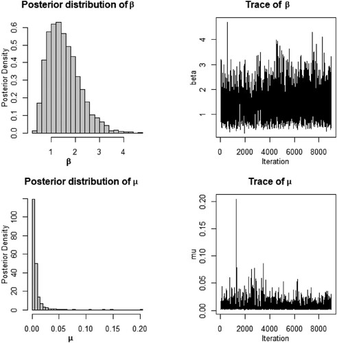
Figure 2. ACF for β.

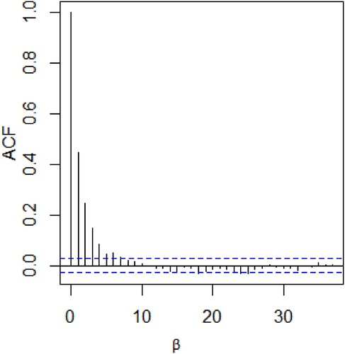
Figure 3. ACF for μ.

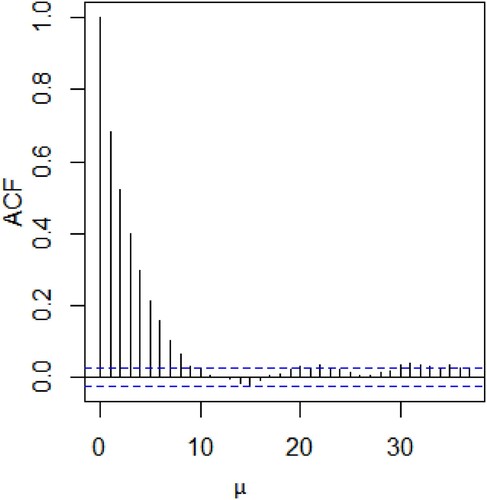
Table 2. Summary of the Bayesian estimates.

Parameter	Median	SD	95% HDI
μ	1.4091	0.6187	(0.5432, 2.7754)
β	0.0042	0.0065	(0.0014, 0.0181)

A clue on the convergence issues on the moments related to the parameter μ is found in simple graphical monitoring like the histogram. Readers may find a similar situation with deviant behaviour or lack of convergence indicators in Example 7.18 (Robert & Casella, 2010). Overall, such graphical indices may serve as a confirmation on the theoretical convergence issues established in Proposition 3.2. for the kth moments of μ, for $k\ge 1$.

4. Conclusion

In this paper, two perspectives have been addressed. First, we have made it clear how objective priors influence the posteriors under record framework for the Weibull model, which is often used as a reliable model with high performances in real data from various aspects. We have noted clear conditions on the objective priors to yield proper posteriors and illustrated their applicability through some well-known prior distributions such as uniform prior, Jeffrey's first rule, Jeffrey's prior, MDIP and reference priors. A relationship between the hyperparameters of the priors and the parameters of the distribution has been used to distinguish proper posteriors from the improper ones. A natural extension on the finitness of the moments of the parameters has been analysed in detail for each of the observed prior. The second perspective of the paper has involved applications of the proposed inference through simulation estimations of posteriors based on real industrial data. Such a study revealed a high level of consistency between theoretical results and real data-based practical realizations.

Acknowledgments

The authors would like to thank anonymous reviewers for their constructive comments.

Disclosure statement

No potential conflict of interest was reported by the author(s).

Additional information

Funding

This research has been supported by the Ministry of Science, Technological Development and Innovation of the Republic of Serbia [contract number 451-03-47/2023-01/200102].

References

- Arnold, B. C., Balakrishnan, N., & Nagaraja, H. N. (2011). Records. John Wiley & Sons.
- Balakrishnan, N., Balasubramanian, K., & Panchapakesan, S. (1996). δ-exceedance records. Journal of Applied Statistical Science, 4(2/3), 123–132.
- Benestad, R. E. (2003). How often can we expect a record event? Climate Research, 25(1), 3–13. https://doi.org/10.3354/cr025003
- Berger, J. O., Bernardo, J. M., & Sun, D. (2015). Overall objective priors. Bayesian Analysis, 10(1), 189–221.
- Bernardo, J. M. (1979). Reference posterior distributions for Bayesian inference. Journal of the Royal Statistical Society: Series B (Methodological), 41(2), 113–128.
- Bernardo, J. M. (2005). Reference analysis. Handbook of Statistics, 25, 17–90. https://doi.org/10.1016/S0169-7161(05)25002-2
- Chandler, K. N. (1952). The distribution and frequency of record values. Journal of the Royal Statistical Society: Series B (Methodological), 14(2), 220–228.
- Doostparast, M. (2011). Goodness-of-fit tests for Weibull populations on the basis of records. arXiv preprint arXiv:1110.5509.
- Dziubdziela, W., & Kopociński, B. (1976). Limiting properties of the kth record values. Applicationes Mathematicae, 15(2), 187–190. https://doi.org/10.4064/am-15-2-187-190
- Empacher, C., Kamps, U., & Volovskiy, G. (2023). Statistical prediction of future sports records based on record values. Stats, 6(1), 131–147. https://doi.org/10.3390/stats6010008
- Gembris, D., Taylor, J. G., & Suter, D. (2007). Evolution of athletic records: Statistical effects versus real improvements. Journal of Applied Statistics, 34(5), 529–545. https://doi.org/10.1080/02664760701234850
- Glick, N. (1978). Breaking records and breaking boards. The American Mathematical Monthly, 85(1), 2–26. https://doi.org/10.1080/00029890.1978.11994501
- Gugushvili, S., & Spreij, P. (2014). Nonparametric Bayesian drift estimation for multidimensional stochastic differential equations. Lithuanian Mathematical Journal, 54(2), 127–141. https://doi.org/10.1007/s10986-014-9232-1
- Hassan, A. S., Nagy, H. F., Muhammed, H. Z., & Saad, M. S. (2020). Estimation of multicomponent stress-strength reliability following Weibull distribution based on upper record values. Journal of Taibah University for Science, 14(1), 244–253. https://doi.org/10.1080/16583655.2020.1721751
- Jafari, A. A., & Bafekri, S. (2021). Inferences on the performance index of Weibull distribution based on k-record values. Journal of Computational and Applied Mathematics, 382, 113060. https://doi.org/10.1016/j.cam.2020.113060
- Juhás, M., & Skřivánková, V. 2014. Characterization of general classes of distributions based on independent property of transformed record values. Applied Mathematics and Computation 226 44–50. https://doi.org/10.1016/j.amc.2013.10.037
- Kang, S. G., Lee, W. D., & Kim, Y. (2017). Noninformative priors for the ratio of the shape parameters of two Weibull distributions. Computational Statistics, 32(1), 35–50. https://doi.org/10.1007/s00180-015-0631-5
- Kass, R. E., & Wasserman, L. (1996). The selection of prior distributions by formal rules. Journal of the American Statistical Association, 91(435), 1343–1370. https://doi.org/10.1080/01621459.1996.10477003
- Kauffman, S., & Levin, S. (1987). Towards a general theory of adaptive walks on rugged landscapes. Journal of Theoretical Biology, 128(1), 11–45. https://doi.org/10.1016/S0022-5193(87)80029-2
- Kim, Y., & Seo, J. I. (2020). objective Bayesian prediction of future record statistics based on the exponentiated Gumbel distribution: Comparison with time-series prediction. Symmetry, 12(9), 1443. https://doi.org/10.3390/sym12091443
- Kizilaslan, F., & Nadar, M. (2017). Statistical inference of P(X<Y) for the Burr Type XII distribution based on records. Hacettepe Journal of Mathematics and Statistics, 46(4), 713–742.
- Lee, W. D., Kang, S. G., & Kim, Y. (2015). Noninformative priors for the common shape parameters of Weibull distributions. Journal of the Korean Statistical Society, 44(4), 668–679. https://doi.org/10.1016/j.jkss.2015.07.003
- Lee, W. D., Kang, S. G., & Kim, Y. (2017). Objective Bayesian inference for the ratio of the scale parameters of two Weibull distributions. Communications in Statistics-Theory and Methods, 46(10), 4943–4956. https://doi.org/10.1080/03610926.2015.1091477
- Liang, F., Paulo, R., Molina, G., Clyde, M. A., & Berger, J. O. (2008). Mixtures of g priors for Bayesian variable selection. Journal of the American Statistical Association, 103(481), 410–423. https://doi.org/10.1198/016214507000001337
- Madadi, M., & Tata, M. (2014). Shannon information in k-records. Communications in Statistics – Theory and Methods, 43(15), 3286–3301. https://doi.org/10.1080/03610926.2012.697965
- Martinez, E. Z., de Freitas, B. C. L., Achcar, J. A., Aragon, D. C., & de Oliveira Peres, M. V. (2022). Exponentiated Weibull models applied to medical data in presence of right-censoring, cure fraction and covariates. Statistics, Optimization & Information Computing, 10(2), 548–571. https://doi.org/10.19139/soic.v10i2
- Nasiri, P., & Hosseini, S. (2012). Statistical inferences for Lomax distribution based on record values (Bayesian and classical). Journal of Modern Applied Statistical Methods, 11(1), 179–189. https://doi.org/10.22237/jmasm/1335845640
- Neal, P., & Roberts, G. (2008). Optimal scaling for random walk Metropolis on spherically constrained target densities. Methodology and Computing in Applied Probability, 10(2), 277–297. https://doi.org/10.1007/s11009-007-9046-2
- Nevzorov, V. B. (2000). Records: Mathematical theory. AMS.
- Northrop, P. J., & Attalides, N. (2016). Posterior propriety in Bayesian extreme value analyses using reference priors. Statistica Sinica, 26(2), 721–743.
- R Core Team (2024). R: A language and environment for statistical computing.
- Ramos, E., Egbon, O. A., Ramos, P. L., Rodrigues, F. A., & Louzada, F. (2020). Objective Bayesian analysis for the differential entropy of the Gamma distribution. arXiv preprint arXiv:2012.14081.
- Ramos, E., Ramos, P. L., & Louzada, F. (2020). Posterior properties of the Weibull distribution for censored data. Statistics & Probability Letters, 166, 108873. https://doi.org/10.1016/j.spl.2020.108873
- Ramos, P. L., Achcar, J. A., Moala, F. A., Ramos, E., & Louzada, F. (2017). Bayesian analysis of the generalized gamma distribution using non-informative priors. Statistics, 51(4), 824–843.
- Ramos, P. L., Almeida, M. H., Louzada, F., Flores, E., & Moala, F. A. (2022). Objective Bayesian inference for the Capability index of the Weibull distribution and its generalization. Computers & Industrial Engineering, 167, 108012. https://doi.org/10.1016/j.cie.2022.108012
- Ramos, P. L., Dey, D. K., Louzada, F., & Ramos, E. (2021). On posterior properties of the two parameter gamma family of distributions. Anais da Academia Brasileira de Ciencias, 93(suppl 3), e20190826. https://doi.org/10.1590/0001-3765202120190826
- Ramos, P. L., Rodrigues, F. A., Ramos, E., Dey, D. K., & Louzada, F. (2023). Power laws distributions in objective priors. Statistica Sinica, 33(3), 1–53.
- Robert, C. P., & Casella, G. (2010). Introducing Monte Carlo methods with R (Vol. 18). Springer.
- Shakhatreh, M. K., Dey, S., & Alodat, M. T. (2021). Objective Bayesian analysis for the differential entropy of the Weibull distribution. Applied Mathematical Modelling, 89, 314–332. https://doi.org/10.1016/j.apm.2020.07.016
- Shakhatreh, M. K., Lemonte, A. J., & Cordeiro, G. M. (2020). On the generalized extended exponential-Weibull distribution: Properties and different methods of estimation. International Journal of Computer Mathematics, 97(5), 1029–1057. https://doi.org/10.1080/00207160.2019.1605062
- Sun, D. (1997). A note on noninformative priors for Weibull distributions. Journal of Statistical Planning and Inference, 61(2), 319–338. https://doi.org/10.1016/S0378-3758(96)00155-3
- Syam, A. H., & Barakat, H. M. (2022). Information measures for record values and their concomitants under Haung-Kotz FGM bivariate distribution. Bulletin of Faculty of Science, Zagazig University, 2022(3), 122–130. https://doi.org/10.21608/bfszu.2022.147965.1154
- Teimouri, M., & Nadarajah, S. (2013). Bias corrected MLEs for the Weibull distribution based on records. Statistical Methodology, 13, 12–24. https://doi.org/10.1016/j.stamet.2013.01.001
- Thornton, C., Hutter, F., Hoos, H. H., & Leyton-Brown, K. (2013). Auto-WEKA: Combined selection and hyperparameter optimization of classification algorithms. In Proceedings of the 19th ACM SIGKDD International Conference on Knowledge Discovery and Data Mining (pp. 847–855).
- Vidović, Z. (2021). Random chord in a circle and Bertrand's paradox: New generation method, extreme behaviour and length moments. Bulletin of the Korean Mathematical Society, 58(2), 433–444.
- Volovskiy, G., & Kamps, U. (2023). Likelihood-based prediction of future Weibull record values. REVSTAT-Statistical Journal, 21(3), 425–445.
- Wang, B. X., & Ye, Z. S. (2015). Inference on the Weibull distribution based on record values. Computational Statistics & Data Analysis, 83, 26–36. https://doi.org/10.1016/j.csda.2014.09.005
- Weibull, W. (1951). A statistical distribution function of wide applicability. Journal of Applied Mechanics, 18(3), 293–297. https://doi.org/10.1115/1.4010337
- Wergen, G. (2013). Records in stochastic processes: Theory and applications. Journal of Physics A: Mathematical and Theoretical, 46(22), 223001. https://doi.org/10.1088/1751-8113/46/22/223001
- Xia, Z. P., Yu, J. Y., Cheng, L. D., Liu, L. F., & Wang, W. M. (2009). Study on the breaking strength of jute fibres using modified Weibull distribution. Composites Part A: Applied Science and Manufacturing, 40(1), 54–59. https://doi.org/10.1016/j.compositesa.2008.10.001
- Zellner, A. (1977). Maximal data information prior distributions. New developments in the applications of Bayesian methods (pp. 211–232). North-Holland.