Variable selection and subgroup analysis for high-dimensional censored data

Abstract

This paper proposes a penalized method for high-dimensional variable selection and subgroup identification in the Tobit model. Based on Olsen's [(1978). Note on the uniqueness of the maximum likelihood estimator for the Tobit model. Econometrica: Journal of the Econometric Society, 46(5), 1211–1215. https://doi.org/10.2307/1911445] convex reparameterization of the Tobit negative log-likelihood, we develop an efficient algorithm for minimizing the objective function by combining the alternating direction method of multipliers (ADMM) and generalised coordinate descent (GCD). We also establish the oracle properties of our proposed estimator under some mild regularity conditions. Furthermore, extensive simulations and an empirical data study are conducted to demonstrate the performance of the proposed approach.

Keywords:

• Tobit model
• fusion
• concave penalty
• oracle property

1. Introduction

Subgroup analysis has broad applicability in precision medicine, economics and sociology as there is an increasing need to distinguish homogeneous subgroups of individuals, detect the subgroup structure and model the relationships between the response variable and predictors for individuals belonging to different subgroups. Thus, vast statistical methods for subgroup analysis have been developed, such as mixture models (Everitt, 2013) and regularization methods (Ma & Huang, 2017). Mixture model methods assume that the data come from a mixture of subgroups and require the specification of an underlying distribution. Shen and He (2015) proposed a structured logistic-normal mixture model to identify subgroups. However, they often require the number of subgroups to be specified to group the parameterized models, which can often be difficult to implement in practice. In contrast, Ma and Huang (2017) developed a pairwise fusion approach using concave penalty functions, such as the smoothly clipped absolute deviation (SCAD, J. Fan & Li, 2001) penalty and the minimax concave penalty (MCP, Zhang, 2010), that automatically identifies subgroup structures and estimates subgroup-specific effects. Ma et al. (2019) considered a heterogeneous treatment effects model. Wang et al. (2019) proposed a general framework of spatial subgroup analysis method for spatial data with repeated measures.

In numerous regression problems, the dependent variables can only be observed within a restricted range. For instance, when studying the influencing factors of different family expenditures in a group, some families may spend zero on items like medical insurance. Similarly, when studying individual or collective income, negative income generated by debt cannot be included in the income calculation. These scenarios involve left-censored data, which exist commonly in economics. Therefore, it encourages us to develop models specially tailored to address such situations. Tobin (1958) developed the Tobit model to study the relationship between the annual expenditure of durable goods and household income. Due to the large number of scenarios of left-censored data in economics and social sciences, the Tobit model remained popular and it has been thoroughly studied and extended to deal with other types of censored data (Amemiya, 1984). Regarding subgroup analysis with censored data, Dagne (2016) proposed a method that simultaneously addresses left-censoring and unobserved heterogeneity within longitudinal data. Additionally, Yan et al. (2021) developed a censored linear regression model with heterogeneous treatment effects.

The advent of advanced data collection techniques has led to an increase in the prevalence of high-dimensional data in the aforementioned fields. When dealing with high-dimensional problems, J. Fan and Lv (2010) provided a comprehensive overview of variable selection approaches, which incorporate methods discussed by J. Fan and Li (2001). In the context of high-dimensional censored models, Müller and van de Geer (2016) and Zhou and Liu (2016) respectively introduced lasso penalty and adaptive lasso penalty to the least absolute deviation (LAD) estimator (Powell, 1984) for variable selection in high-dimensional censored models. Johnson (2009) and Soret et al. (2018) proposed lasso penalties for Buckley-James estimators in right and left censored data. Moreover, Bradic et al. (2011) provided a non-concave penalized approach in Cox proportional hazards model with non-polynomial-dimensionality. Alhamzawi (2016) and Alhamzawi (2020) developed the Bayesian method of penalty censored regression. Recently, Jacobson and Zou (2023) extended the Tobit model to high-dimensional regression. However, none of these methods focus on subgroup analysis in high-dimensional censored data.

This paper focuses on subgroup identification and variable selection for a high-dimensional Tobit model. To the best of our knowledge, there have been no discussions on subgroup analysis for high-dimensional Tobit models in the existing literature. We adopt a penalized approach to identify the subgroup structures and select covariates simultaneously. The subgroup structure is determined by penalizing pairwise differences between subject-specific effects while significant covariates are chosen based on a penalty on coefficients. To ensure the sparsity and unbiasedness of the proposed estimators, we consider two commonly used concave penalties, SCAD (J. Fan & Li, 2001) and MCP (Zhang, 2010). Due to the non-convex of the negative log-likelihood in the Tobit model (Tobin, 1958), optimization becomes challenging for high-dimensional settings. To address this issue, we employ a convex reparameterization of negative log-likelihood, building upon the idea proposed by Olsen (1978). This reparameterization enables us to solve the problem using convex optimization approaches. The computational algorithm we proposed combines the alternating direction method of multipliers (ADMM) algorithm (Boyd et al., 2011) and generalized coordinate descent (GCD) algorithm (Jacobson & Zou, 2023; Yang & Zou, 2013) using two concave penalties, such as SCAD or MCP. Furthermore, we conduct a theoretical analysis of the proposed estimators and establish their oracle properties under mild conditions.

The remainder of this paper is organized as follows. Section 2 introduces the main problem and outlines the proposed method. In Section 3, we propose an algorithm for identifying the subgroup structures and performing variable selection. We state technical assumptions and establish the theoretical properties of our proposed approach in Section 4. Section 5 provides extensive simulation studies to illustrate the empirical performance of the proposed method, while Section 6 presents its application to empirical data. A summary and prospects for future research are presented in Section 7 and all technical proofs are given in Appendix.

2. Model and method

2.1. Model setting

Suppose that ${\mathbf{x}}_i=(x_{i1},\dots ,x_{\mathrm{ip}}{)}^{\mathrm{\top }}$ is a p-dimensional vector of covariates for the ith subject. $y_i\ge c$ is the response for a restricted range, where c is a known constant. Without loss of generality, we assume that c = 0 in the following. The Tobit model assumes that the observed data y satisfies $y=max(y^{\ast },c)$, where $y^{\ast }$ is a latent variable. Under the homogeneous case, the classical linear model takes the form (1) $\begin{array}{r}{y}_i^{\ast }=\mu +{\mathbf{x}}_i^{\mathrm{\top }}\mathit{\beta }+{ϵ}_i,i=1,\dots ,n,\end{array}$(1) where μ is the unknown intercept, $\mathit{\beta }=({\beta }_1,\dots ,{\beta }_p{)}^{\mathrm{\top }}$ is the vector of coefficients for the covariates ${\mathbf{x}}_i$, and ${ϵ}_i$ are assumed to be independent and identically distributed with normal distribution $N(0,{\sigma }^2)$.

If individuals are from different groups with a unique intercept ${\mu }_i$, the homogeneity assumption in the model (1(1) $\begin{array}{r}{y}_i^{\ast }=\mu +{\mathbf{x}}_i^{\mathrm{\top }}\mathit{\beta }+{ϵ}_i,i=1,\dots ,n,\end{array}$(1) ) is invalid. To model the subject-specific effects, we consider the subject-specific linear model (2) $\begin{array}{r}{y}_i^{\ast }={\mu }_i+{\mathbf{x}}_i^{\mathrm{\top }}\mathit{\beta }+{ϵ}_i,i=1,\dots ,n.\end{array}$(2) We assume $(y_1^{\ast },\dots ,y_n^{\ast })$ arise from $K$ different groups with $K\ge 1$ unknown and the subjects from the same groups have the same intercept. In other words, we have ${\mu }_i={\pi }_k$ for all $i\in {\mathcal{G}}_k$, where ${\pi }_k$ is the common value of intercept ${\mu }_i$ in subgroup ${\mathcal{G}}_k$ and $\mathcal{G}=({\mathcal{G}}_1,\dots ,{\mathcal{G}}_K)$ is a mutually partition of $\{1,\dots ,n\}$. In practice, the number of subgroups K is unknown and is smaller than the sample size n.

Define $d_i=I(y_i\ge 0)$, where $I(\cdot )$ is an indicator function. Then the observed data $(y_1,\dots ,y_n)$ satisfy the following Tobit model (3) $\begin{array}{r}{y}_i=d_i{y}_i^{\ast }=\{\begin{array}{ll}{\mu }_i+{\mathbf{x}}_i\mathit{\beta }+{ϵ}_i,& \text{if}{y}_i^{\ast }\ge 0,\\ 0,& \text{if}{y}_i^{\ast }<0,\end{array}i=1,\dots ,n,\end{array}$(3) with subgroup structure (4) $\begin{array}{r}{\mu }_i=\{\begin{array}{ll}{\pi }_1,& \text{if}i\in {\mathcal{G}}_1,\\ {\pi }_2,& \text{if}i\in {\mathcal{G}}_2,\\ ⋮& ⋮\\ {\pi }_K,& \text{if}i\in {\mathcal{G}}_K.\end{array}\end{array}$(4) Let $\mathrm{\Phi }(\cdot )$ denote the standard normal cumulative distribution function (CDF). Then $P(y_i^{\ast }\le 0)=P({\mu }_i+{\mathbf{x}}_i^{\mathrm{\top }}\mathit{\beta }<0)=\mathrm{\Phi }(-\frac{{\mu }_i+{\mathbf{x}}_i^{\mathrm{\top }}\mathit{\beta }}{\sigma }),$and the Tobit likelihood is given by $L_n(\mathit{\mu }\mathbf{,}\mathit{\beta },{\sigma }^2)=\prod _{i=1}^n{[\frac{1}{\sqrt{2\pi }\sigma }\exp \{-\frac{1}{2{\sigma }^2}(y_i-{\mu }_i-{\mathbf{x}}_i^{\mathrm{\top }}\mathit{\beta }{)}^2\}]}^{d_i}{\left[\mathrm{\Phi }\left(\frac{-{\mu }_i-{\mathbf{x}}_i^{\mathrm{\top }}\mathit{\beta }}{\sigma }\right)\right]}^{1-d_i},$where $\mathit{\mu }=({\mu }_1,\dots ,{\mu }_n{)}^{\mathrm{\top }}$. Therefore, after omitting an inconsequential constant, the log-likelihood function of the Tobit model is $\begin{array}{rl}\log L_n(\mathit{\mu },\mathit{\beta },{\sigma }^2)& =\sum _{i=1}^n(d_i[-\frac{1}{2}(y_i-{\mu }_i-{\mathbf{x}}_i^{\mathrm{\top }}\mathit{\beta }{)}^2/{\sigma }^2-\log (\sigma )]\\ & +(1-d_i)\log \left[\mathrm{\Phi }(-\frac{{\mu }_i+{\mathbf{x}}_i^{\mathrm{\top }}\mathit{\beta }}{\sigma })\right]).\end{array}$It is apparent that the function $\log L_n(\mathit{\mu },\mathit{\beta },{\sigma }^2)$ is non-concave with respect to the parameters $(\mathit{\mu },\mathit{\beta },{\sigma }^2)$. By adopting the reparameterization suggested in the works of Olsen (1978) and Jacobson and Zou (2023) with $\mathit{\delta }=\mathit{\beta }/\sigma$, ${\alpha }_i={\mu }_i/\sigma$ and ${\gamma }^2={\sigma }^{-2}$, we achieve a transformation that leads to a concave function with respect to parameters $(\mathit{\alpha },\mathit{\delta },\gamma )$, $\log L_n(\mathit{\alpha }\mathbf{,}\mathit{\delta },\gamma )=\sum _{i=1}^n\{d_i[\log (\gamma )-\frac{1}{2}(\gamma y_i-{\alpha }_i-{\mathbf{x}}_i^{\mathrm{\top }}\mathit{\delta }{)}^2]+(1-d_i)\log (\mathrm{\Phi }(-{\alpha }_i-{\mathbf{x}}_i^{\mathrm{\top }}\mathit{\delta }))\},$where $\mathit{\alpha }=({\alpha }_1,\dots ,{\alpha }_n{)}^{\mathrm{\top }}$.

2.2. Method

There are usually some redundant covariates in high-dimensional scenarios, and regularization is the most commonly used method to identify the sparsity of regression coefficient vectors (Bondell & Reich, 2008; J. Fan & Lv, 2010; Y. Fan & Tang, 2013). The subgroup structure (4(4) $\begin{array}{r}{\mu }_i=\{\begin{array}{ll}{\pi }_1,& \text{if}i\in {\mathcal{G}}_1,\\ {\pi }_2,& \text{if}i\in {\mathcal{G}}_2,\\ ⋮& ⋮\\ {\pi }_K,& \text{if}i\in {\mathcal{G}}_K.\end{array}\end{array}$(4) ) can be transformed as the fusion sparse structure, ${\alpha }_i-{\alpha }_j=({\mu }_i-{\mu }_j)/\sigma =0(i,j\in {\mathcal{G}}_k,k=1,\dots ,K)$. In order to estimate the parameters $\mathit{\alpha },\mathit{\delta }$, and γ, and to select proper covariates through the sparsity assumption of $\mathit{\delta }$, we propose a new method that combines ideas of penalized Tobit regression (Jacobson & Zou, 2023) and the subgroup analysis by concave pairwise fusion penalization (Ma & Huang, 2017; Ma et al., 2019), which can be expressed as minimizing the following loss function (5) $\begin{array}{r}Q(\mathit{\alpha }\mathbf{,}\mathit{\delta },\gamma ;{\lambda }_1,{\lambda }_2)=-\frac{1}{n}\log L_n(\mathit{\alpha }\mathbf{,}\mathit{\delta },\gamma )+\sum _{i=1}^p{P}_{{\lambda }_1}(|{\delta }_i|)+\sum _{i<j}{P}_{{\lambda }_2}(|{\alpha }_i-{\alpha }_j|),\end{array}$(5) where $P_{{\lambda }_1}(\cdot )$ and $P_{{\lambda }_2}(\cdot )$ are penalty functions, ${\lambda }_1,{\lambda }_2\ge 0$ are tuning parameters that control the strengths of regularization of $|{\delta }_i|$ and $|{\alpha }_i-{\alpha }_j|$, respectively. Note that the sparsity of $\mathit{\delta }$ is achieved through the first penalty term, while the homogeneity detection is achieved by the second penalty term. Additionally, when ${\lambda }_1=0$ the problem reduces to the subgroup analysis in censored regression; when ${\lambda }_2=0$ the problem reduces to the penalized Tobit regression.

It is important to note that lasso estimators may fail to achieve consistent model selection unless a stringent ‘irrepresentable condition’ (Zhao & Yu, 2006; Zou, 2006). Particularly, the $L_1$ penalty tends to overshrink non-zero difference of $|{\alpha }_i-{\alpha }_j|$, which can result in an inflated number of subgroups. To address this limitation, we consider two common concave penalty functions for the purposes of identifying the subgroup structure and selecting variables, namely the smoothly clipped absolute deviation (SCAD, J. Fan & Li, 2001) and the minimax concave penalty (MCP, Zhang, 2010). These penalties provide alternative approaches to handle the challenges associated with variable selection and subgroup detection.

The SCAD is defined as follows $P_{\lambda }(t)=\lambda {\int }_0^{t}I(x\le \lambda )+\frac{(\mathrm{a\lambda }-x{)}_{+}}{(a-1)\lambda }I(x>\lambda )\mathrm{d}x,a>2,$and the MCP is $P_{\lambda }(t)={\int }_0^t\frac{(\mathrm{a\lambda }-x{)}_{+}}{a}\mathrm{d}x,a>1,$where a is a parameter that controls the concavity of the penalty function.

3. Computational algorithm

In this section, we propose an algorithm utilizing the alternating direction method of multipliers (ADMM) (Boyd et al., 2011) in conjunction with generalized coordinate descent (GCD) (Jacobson & Zou, 2023; Yang & Zou, 2013) to address the minimization problem (5(5) $\begin{array}{r}Q(\mathit{\alpha }\mathbf{,}\mathit{\delta },\gamma ;{\lambda }_1,{\lambda }_2)=-\frac{1}{n}\log L_n(\mathit{\alpha }\mathbf{,}\mathit{\delta },\gamma )+\sum _{i=1}^p{P}_{{\lambda }_1}(|{\delta }_i|)+\sum _{i<j}{P}_{{\lambda }_2}(|{\alpha }_i-{\alpha }_j|),\end{array}$(5) ). Since the penalty function is not separable with respect to ${\alpha }_i$, it is challenging to directly minimize the objective function (5(5) $\begin{array}{r}Q(\mathit{\alpha }\mathbf{,}\mathit{\delta },\gamma ;{\lambda }_1,{\lambda }_2)=-\frac{1}{n}\log L_n(\mathit{\alpha }\mathbf{,}\mathit{\delta },\gamma )+\sum _{i=1}^p{P}_{{\lambda }_1}(|{\delta }_i|)+\sum _{i<j}{P}_{{\lambda }_2}(|{\alpha }_i-{\alpha }_j|),\end{array}$(5) ). We introduce a new set of parameters ${\eta }_{\mathrm{ij}}={\alpha }_i-{\alpha }_j$, and then the minimizing problem can be written as the following constraint optimization problem $\begin{array}{rl}S(\mathit{\alpha }\mathbf{,}\mathit{\delta }\mathbf{,}\mathit{\eta },\gamma ;{\lambda }_1,{\lambda }_2)& ={\ell }_n(\mathit{\alpha }\mathbf{,}\mathit{\delta },\gamma )+\sum _{i=1}^p{P}_{{\lambda }_1}(|{\delta }_i|)+\sum _{i<j}{P}_{{\lambda }_2}(|{\eta }_{\mathrm{ij}}|),\\ & \text{subject to}{\alpha }_i-{\alpha }_j-{\eta }_{\mathrm{ij}}=0,\end{array}$where ${\ell }_n(\mathit{\alpha }\mathbf{,}\mathit{\delta },\gamma )=-\frac{1}{n}\log L_n(\mathit{\alpha }\mathbf{,}\mathit{\delta },\gamma )$ is the negative log-likelihood function which we call it Tobit loss for short and $\mathit{\eta }=\{{\eta }_{\mathrm{ij}},i<j{\}}^{\mathrm{\top }}$. Applying the augmented Lagrangian method, the estimates of the parameters can be obtained by minimizing (6) $\begin{array}{r}L(\mathit{\alpha }\mathbf{,}\mathit{\delta }\mathbf{,}\mathit{\eta }\mathbf{,}\mathit{\phi },\gamma ;{\lambda }_1,{\lambda }_2,\rho )=S(\mathit{\alpha }\mathbf{,}\mathit{\delta }\mathbf{,}\mathit{\eta },\gamma ;{\lambda }_1,{\lambda }_2)+\sum _{i<j}{\phi }_{\mathrm{ij}}({\alpha }_i-{\alpha }_j-{\eta }_{\mathrm{ij}})+\frac{\rho }{2}\sum _{i<j}({\alpha }_i-{\alpha }_j-{\eta }_{\mathrm{ij}}{)}^2,\end{array}$(6) where $\mathit{\phi }=\{{\phi }_{\mathrm{ij}},i<j{\}}^{\mathrm{\top }}$ are Lagrange multipliers, and ρ is the penalty parameter.

To obtain the minimum in (6(6) $\begin{array}{r}L(\mathit{\alpha }\mathbf{,}\mathit{\delta }\mathbf{,}\mathit{\eta }\mathbf{,}\mathit{\phi },\gamma ;{\lambda }_1,{\lambda }_2,\rho )=S(\mathit{\alpha }\mathbf{,}\mathit{\delta }\mathbf{,}\mathit{\eta },\gamma ;{\lambda }_1,{\lambda }_2)+\sum _{i<j}{\phi }_{\mathrm{ij}}({\alpha }_i-{\alpha }_j-{\eta }_{\mathrm{ij}})+\frac{\rho }{2}\sum _{i<j}({\alpha }_i-{\alpha }_j-{\eta }_{\mathrm{ij}}{)}^2,\end{array}$(6) ), we propose to use the following iterative algorithm based on the ADMM. Let t denote the iteration step. We update the estimates of $(\mathit{\alpha },\mathit{\delta },\gamma )$, $\mathit{\eta }$, and $\mathit{\phi }$ iteratively at the $(t+1)$th iteration step as follows (7) $\begin{array}{rl}({\mathit{\alpha }}^{(t+1)},{\mathit{\delta }}^{(t+1)},{\gamma }^{(t+1)})& =\arg \underset{\mathit{\delta },\mathit{\alpha },\gamma }{min}L(\mathit{\alpha },\mathit{\delta },\gamma ,{\mathit{\eta }}^{(t)},{\mathit{\phi }}^{(t)}),\end{array}$(7) (8) $\begin{array}{rl}{\mathit{\eta }}^{(t+1)}& =\arg \underset{\mathit{\eta }}{min}L({\mathit{\alpha }}^{(t+1)},{\mathit{\delta }}^{(t+1)},{\gamma }^{(t+1)},\mathit{\eta },{\mathit{\phi }}^{(t)}),\end{array}$(8) (9) $\begin{array}{rl}{\mathit{\phi }}^{(t+1)}& ={\mathit{\phi }}^{(t)}+\rho (\mathrm{\Delta }{\mathit{\alpha }}^{(t+1)}-{\mathit{\eta }}^{(t+1)}),\end{array}$(9) where $\mathrm{\Delta }=\{(e_i-e_j),i<j{\}}^{\mathrm{\top }}$.

It is worth noting that, given $({\mathit{\eta }}^{(t)},{\mathit{\phi }}^{(t)})$, the objective function in the first minimization problem (7(7) $\begin{array}{rl}({\mathit{\alpha }}^{(t+1)},{\mathit{\delta }}^{(t+1)},{\gamma }^{(t+1)})& =\arg \underset{\mathit{\delta },\mathit{\alpha },\gamma }{min}L(\mathit{\alpha },\mathit{\delta },\gamma ,{\mathit{\eta }}^{(t)},{\mathit{\phi }}^{(t)}),\end{array}$(7) ) can be simplified as (10) $\begin{array}{rl}L(\mathit{\alpha },\mathit{\delta },\gamma ,\mathit{\eta },\mathit{\phi })& =\frac{1}{n}\sum _{i=1}^n{\ell }_i({\alpha }_i,\mathit{\delta },\gamma )+\sum _{i=1}^p{P}_{{\lambda }_1}(|{\delta }_i|)+\sum _{i<j}{\phi }_{\mathrm{ij}}({\alpha }_i-{\alpha }_j-{\eta }_{\mathrm{ij}})\\ & +\frac{\rho }{2}\sum _{i<j}({\alpha }_i-{\alpha }_j-{\eta }_{\mathrm{ij}}{)}^2+C,\end{array}$(10) where ${\ell }_i({\alpha }_i,\mathit{\delta },\gamma )=\frac{1}{2}{d}_i(\gamma y_i-{\alpha }_i-{\mathbf{x}}_i^{\mathrm{\top }}\mathit{\delta }{)}^2-(1-d_i)\log \mathrm{\Phi }(-{\mathbf{x}}_i^{\mathrm{\top }}\mathit{\delta }-{\alpha }_i))$, and C is a constant independent with $(\mathit{\alpha }\mathbf{,}\mathit{\delta },\gamma )$.

Due to the complexity of the function (10(10) $\begin{array}{rl}L(\mathit{\alpha },\mathit{\delta },\gamma ,\mathit{\eta },\mathit{\phi })& =\frac{1}{n}\sum _{i=1}^n{\ell }_i({\alpha }_i,\mathit{\delta },\gamma )+\sum _{i=1}^p{P}_{{\lambda }_1}(|{\delta }_i|)+\sum _{i<j}{\phi }_{\mathrm{ij}}({\alpha }_i-{\alpha }_j-{\eta }_{\mathrm{ij}})\\ & +\frac{\rho }{2}\sum _{i<j}({\alpha }_i-{\alpha }_j-{\eta }_{\mathrm{ij}}{)}^2+C,\end{array}$(10) ) with respect to $(\mathit{\alpha }\mathbf{,}\mathit{\delta },\gamma )$, we apply the generalized coordinate descent (GCD) method to solve the problem. By employing the GCD method, we can iteratively update each variable while holding the others fixed.

Let ${\mathit{\alpha }}^{\prime },{\mathit{\delta }}^{\prime }$ and ${\gamma }^{\prime }$ be the current values for $\mathit{\alpha },\mathit{\delta }$ and γ, respectively. For the sake of simplicity in notation, let ${\mathbf{v}}_{(-j)}$ denote the vector $\mathbf{v}$ with the jth element removed in the subsequent context. In order to get the estimate of ${\alpha }_i$, we begin by expressing the Tobit loss ${\ell }_n$ with respect to ${\alpha }_i$ ${\ell }_n({\alpha }_i\mid {\mathit{\alpha }}_{(-i)}^{\prime },{\mathit{\delta }}^{\prime },{\gamma }^{\prime })=\frac{1}{n}\{\frac{1}{2}{d}_i(\gamma y_i-{\alpha }_i-{\mathbf{x}}_i^{\mathrm{\top }}{\mathit{\delta }}^{\prime }{)}^2-(1-d_i)\log \mathrm{\Phi }(-{\mathbf{x}}_i^{\mathrm{\top }}{\mathit{\delta }}^{\prime }-{\alpha }_i)\}.$We observe that after dropping the negligible constants, the Tobit loss ${\ell }_n$ associated with ${\alpha }_i$ solely depends on the data collected from subject i. In line with Theorem 1 presented in Jacobson and Zou (2023), the quadratic majorization function for ${\ell }_n({\alpha }_i\mid {\mathit{\alpha }}^{\prime },{\mathit{\delta }}^{\prime },{\gamma }^{\prime })$ takes the following form: $Q_{\alpha }({\alpha }_i\mid {\mathit{\alpha }}_{(-i)}^{\prime },{\mathit{\delta }}^{\prime },{\gamma }^{\prime })={\ell }_n({\alpha }_i^{\prime }\mid {\mathit{\delta }}^{\prime },{\gamma }^{\prime })+{\dot{\ell }}_n({\alpha }_i^{\prime }\mid {\mathit{\delta }}^{\prime },{\gamma }^{\prime })({\alpha }_i-{\alpha }_i^{\prime })+\frac{1}{2}({\alpha }_i-{\alpha }_i^{\prime }{)}^2,$where ${\dot{\ell }}_n({\alpha }_i^{\prime }\mid {\mathit{\delta }}^{\prime },{\gamma }^{\prime })$ represents the derivative of function with respect to ${\alpha }_i$. Following the MM principle, the update of ${\alpha }_i$ can be obtained by minimizing the expression $Q_{\alpha }({\alpha }_i\mid {\mathit{\alpha }}_{(-i)}^{\prime },{\mathit{\delta }}^{\prime },{\gamma }^{\prime })+\frac{\rho }{2}\sum _{k<j}\{(e_k-e_j{)}^{\mathrm{\top }}\mathit{\alpha }-{\eta }_{\mathrm{kj}}+{\rho }^{-1}{\phi }_{\mathrm{kj}}{\}}^2$, and $e_j$ is an $n\times 1$ vector with the jth element being 1 and the remaining elements being 0. Therefore, for fixed ${\mathit{\alpha }}^{(t,k)},{\mathit{\delta }}^{(t,k)}$, and ${\gamma }^{(t,k)}$ at the kth step, the update of ${\mathit{\alpha }}^{(t,k+1)}$ is as follows (11) $\begin{array}{r}{\mathit{\alpha }}^{(t,k+1)}=(I+\mathrm{n\rho }{\mathrm{\Delta }}^{\mathrm{\top }}\mathrm{\Delta }{)}^{-1}(\mathrm{n\rho }{\mathrm{\Delta }}^{\mathrm{\top }}{\mathit{\eta }}^{(t)}-n{\mathrm{\Delta }}^{\mathrm{\top }}{\mathit{\phi }}^{(t)}+{\mathbf{a}}^{(t,k)}),\end{array}$(11) where I is the identity matrix, and ${\mathbf{a}}^{(t,k)}={\mathit{\alpha }}^{(t,k)}-{\dot{\ell }}_n({\mathit{\alpha }}^{(t,k)})$ with ${\dot{\ell }}_n({\mathit{\alpha }}^{(t,k)})=({\dot{\ell }}_n({\alpha }_1^{(t,k)}),\dots ,{\dot{\ell }}_n({\alpha }_n^{(t,k)}){)}^{\mathrm{\top }}$.

Now we consider coordinate-wise updates of ${\delta }_j,j=1,\dots ,p$. Let $M_j=\frac{1}{n}\sum _{i=1}^n{x}_{\mathrm{ij}}^2$. Similarly to ${\alpha }_i$, we also have the quadratic majorization function of ${\ell }_n({\delta }_j\mid {\mathit{\alpha }}^{\prime },{\mathit{\delta }}^{\prime },{\gamma }^{\prime })$ with respect to ${\delta }_j$ with form $Q_{\delta }({\delta }_j\mid {\mathit{\alpha }}^{\prime },{\mathit{\delta }}_{-j}^{\prime },{\gamma }^{\prime })={\ell }_n({\delta }_j^{\prime }\mid {\mathit{\alpha }}^{\prime },{\mathit{\delta }}_{(-j)}^{\prime },{\gamma }^{\prime })+{\dot{\ell }}_n({\delta }_j^{\prime }\mid {\mathit{\alpha }}^{\prime },{\mathit{\delta }}_{(-j)}^{\prime },{\gamma }^{\prime })({\delta }_j-{\delta }_j^{\prime })+\frac{M_j}{2}({\delta }_j-{\delta }_j^{\prime }{)}^2,$where ${\dot{\ell }}_n({\delta }_j^{\prime }\mid {\mathit{\alpha }}^{\prime },{\mathit{\delta }}_{(-j)}^{\prime },{\gamma }^{\prime })$ is the derivative of ${\ell }_n({\delta }_j\mid {\mathit{\alpha }}^{\prime },{\mathit{\delta }}_{(-j)}^{\prime },{\gamma }^{\prime })$ with respect to ${\delta }_j$. Here, the Tobit loss with respect to ${\delta }_j$ can be expressed as $\begin{array}{rl}{\ell }_n({\delta }_j\mid {\mathit{\alpha }}^{\prime },{\mathit{\delta }}_{(-j)}^{\prime },{\gamma }^{\prime })& =\frac{1}{n}\sum _{i=1}^n\frac{1}{2}{d}_i(\gamma y_i-{\alpha }_i^{\prime }-{\mathbf{x}}_{i,(-j)}^{\mathrm{\top }}{\mathit{\delta }}_{(-j)}^{\prime }-x_{\mathrm{ij}}{\delta }_j{)}^2\\ & -(1-d_i)\log \mathrm{\Phi }(-{\mathbf{x}}_{i,(-j)}{)}^{\mathrm{\top }}{\mathit{\delta }}_{(-j)}^{\prime }-{\alpha }_i^{\prime }-x_{\mathrm{ij}}{\delta }_j)).\end{array}$We can update ${\delta }_j$ by minimizing $Q_{\delta }({\delta }_j\mid {\mathit{\alpha }}^{\prime },{\mathit{\delta }}_{-j}^{\prime },{\gamma }^{\prime })+P_{{\lambda }_1}({\delta }_j)$ through MM principle. For $j=1,\dots ,p$, let ${\upsilon }_j^{(t,k)}={\delta }_j^{(t,k)}-\frac{1}{M_j}{\ell }_n^{\prime }({\delta }_j^{(t,k)}\mid {\mathit{\alpha }}^{(t,k+1)},{\mathit{\delta }}^{(t,k)},{\gamma }^{(t,k)})$. Hence, for SCAD penalty with $a_1>\underset{j}{max}\{M_j^{-1}\}+1$, the update of ${\delta }_j$ at the $(k+1)$th step is (12) $\begin{array}{r}{\delta }_j^{(t,k+1)}=\{\begin{array}{ccl}{\displaystyle \mathrm{ST}({\upsilon }_j^{(t,k)},\frac{{\lambda }_1}{M_j}),}& \text{if}& |{\upsilon }_j^{(t,k)}|\le {\lambda }_1+{\lambda }_1/M_j,\\ {\displaystyle \frac{\mathrm{ST}({\upsilon }_j^{(t,k)},a_1{\lambda }_1/((a_1-1)M_j))}{1-((a_1-1)M_j{)}^{-1}},}& \text{if}& {\lambda }_1+{\lambda }_1/M_j<|{\upsilon }_j^{(t,k)}|\le a_1{\lambda }_1,\\ {\upsilon }_j^{(t,k)},& \text{if}& |{\upsilon }_j^{(t,k)}|>a_1{\lambda }_1,\end{array}\end{array}$(12) where $\mathrm{ST}(t,\lambda )=\text{sign}(t)(|t|-\lambda {)}_{+}$ is the soft-thresholding rule, and $(x{)}_{+}=max\{x,0\}$. And when $a_1>\underset{j}{max}\{M_j^{-1}\}$ for the MCP penalty, the updated value is (13) $\begin{array}{r}{\delta }_j^{(t,k+1)}=\{\begin{array}{ccl}{\displaystyle \frac{\mathrm{ST}({\upsilon }_j^{(t,k)},{\lambda }_1/M_j)}{1-(a_1{M}_j{)}^{-1}},}& \text{if}& |{\upsilon }_j^{(t,k)}|\le a_1{\lambda }_1,\\ {\upsilon }_j^{(t,k)},& \text{if}& |{\upsilon }_j^{(t,k)}|>a_1{\lambda }_1.\end{array}\end{array}$(13) Lastly, for given ${\mathit{\alpha }}^{(t,k+1)}$ and ${\mathit{\delta }}^{(t,k+1)}$, we minimize ${\ell }_n(\gamma \mid {\mathit{\alpha }}^{(t,k+1)},{\mathit{\delta }}^{(t,k+1)})$ to update γ, (14) $\begin{array}{rl}& {\gamma }^{(t,k+1)}\\ & =\frac{\sum _{i=1}^n{d}_i{y}_i({\alpha }_i^{(t,k+1)}+{\mathbf{x}}_i^{\mathrm{\top }}{\mathit{\delta }}^{(t,k+1)})+\sqrt{{(\sum _{i=1}^n{d}_i{y}_i({\alpha }_i^{(t,k+1)}+{\mathbf{x}}_i^{\mathrm{\top }}{\mathit{\delta }}^{(t,k+1)}))}^2+4\left(\sum _{i=1}^n{d}_i{y}_i^2\right)\sum _{i=1}^n{d}_i}}{2\sum _{i=1}^n{d}_i{y}_i^2}.\end{array}$(14) Once the convergence is achieved, we denote the final iteration of the GCD as $({\mathit{\alpha }}^{(t+1)},{\mathit{\delta }}^{(t+1)},{\gamma }^{(t+1)})$.

As for the second minimization function (8(8) $\begin{array}{rl}{\mathit{\eta }}^{(t+1)}& =\arg \underset{\mathit{\eta }}{min}L({\mathit{\alpha }}^{(t+1)},{\mathit{\delta }}^{(t+1)},{\gamma }^{(t+1)},\mathit{\eta },{\mathit{\phi }}^{(t)}),\end{array}$(8) ), by eliminating insignificant constants that have no effect on the minimization process, the optimization function simplifies to the following form (15) $\begin{array}{r}{\eta }_{\mathrm{ij}}=\arg \underset{{\eta }_{\mathrm{ij}}}{min}\frac{\rho }{2}({\eta }_{\mathrm{ij}}-{\zeta }_{\mathrm{ij}}{)}^2+P_{{\lambda }_2}(|{\eta }_{\mathrm{ij}}|),\end{array}$(15) with respect to ${\eta }_{\mathrm{ij}}$, where ${\zeta }_{\mathrm{ij}}={\alpha }_i-{\alpha }_j+{\rho }^{-1}{\phi }_{\mathrm{ij}}$. It's worth noting that (15(15) $\begin{array}{r}{\eta }_{\mathrm{ij}}=\arg \underset{{\eta }_{\mathrm{ij}}}{min}\frac{\rho }{2}({\eta }_{\mathrm{ij}}-{\zeta }_{\mathrm{ij}}{)}^2+P_{{\lambda }_2}(|{\eta }_{\mathrm{ij}}|),\end{array}$(15) ) is convex with respect to each ${\eta }_{\mathrm{ij}}$ when $a_2>{\rho }^{-1}$ for MCP or $a_2>{\rho }^{-1}+1$ for SCAD. Hence, the closed-form solution for the MCP penalty at the $(t+1)$ iteration is (16) $\begin{array}{r}{\eta }_{\mathrm{ij}}^{(t+1)}=\{\begin{array}{ccl}{\displaystyle \frac{\mathrm{ST}({\zeta }_{\mathrm{ij}}^{(t+1)},{\lambda }_2/\rho )}{1-(a_2\rho {)}^{-1}},}& \text{if}& |{\zeta }_{\mathrm{ij}}^{(t+1)}|\le a_2{\lambda }_2,\\ {\zeta }_{\mathrm{ij}}^{(t+1)},& \text{if}& |{\zeta }_{\mathrm{ij}}^{(t+1)}|>a_2{\lambda }_2.\end{array}\end{array}$(16) Then for the SCAD penalty, it is (17) $\begin{array}{r}{\eta }_{\mathrm{ij}}^{(t+1)}=\{\begin{array}{ccl}\mathrm{ST}({\zeta }_{\mathrm{ij}}^{(t+1)},{\lambda }_2/\rho ),& \text{if}& |{\zeta }_{\mathrm{ij}}^{t+1}|\le {\lambda }_2+{\lambda }_2/\rho ,\\ {\displaystyle \frac{\mathrm{ST}({\zeta }_{\mathrm{ij}}^{(t+1)},a_2{\lambda }_2/((a_2-1)\rho ))}{1-((a_2-1)\rho {)}^{-1}},}& \text{if}& {\lambda }_2+{\lambda }_2/\rho <|{\zeta }_{\mathrm{ij}}^{(t+1)}|\le a_2{\lambda }_2,\\ {\zeta }_{\mathrm{ij}}^{(t+1)},& \text{if}& |{\zeta }_{\mathrm{ij}}|>a_2{\lambda }_2.\end{array}\end{array}$(17) We provide the complete algorithm in Algorithm (1), referred to as the ADMM-GCD algorithm for convenience.

Remark

In the algorithm, there are two iterative steps. In the nested GCD iteration, the iterative convergence criterion is defined as follows ${\Vert {({\mathit{\alpha }}^{(t,k+1)}-{\mathit{\alpha }}^{(t,k)})}^{\mathrm{\top }},{({\mathit{\delta }}^{(t,k+1)}-{\mathit{\delta }}^{(t,k)})}^{\mathrm{\top }},({\gamma }^{(t,k+1)}-{\gamma }^{(t,k)})\Vert }_2^2\le {ϵ}_a.$On the other hand, for ADMM, we employ the following criterion $\Vert {\mathbf{r}}^{(t+1)}{\Vert }^2=\Vert \mathbf{\Delta }{\mathit{\alpha }}^{(t+1)}-{\mathit{\eta }}^{(t+1)}{\Vert }_2^2<{ϵ}_b.$It is worth mentioning that in our simulation studies, we set ${ϵ}_a={10}^{-4}$ and ${ϵ}_b={10}^{-5}$, respectively.

The following Proposition 3.1 presents the convergence properties of the proposed algorithm.

Proposition 3.1

Given $a_1>max\{1/M_j\}$ and $a_2>1/\rho$ for MCP or $a_1>max\{1/M_j\}+1$ and $a_2>1/\rho +1$ for SCAD, any accumulation point $({\mathit{\delta }}^{(t+1)},{\mathit{\alpha }}^{(t+1)},{\gamma }^{(t+1)},{\mathit{\eta }}^{(t+1)})$ generated by Algorithm 1 is a coordinate-wise minimum of $L(\mathit{\delta }\mathbf{,}\mathit{\alpha },\gamma ,\mathit{\eta },{\mathit{\phi }}^{(t)})$. In addition, the primal residual ${\mathbf{r}}^{(t+1)}=\mathrm{\Delta }{\mathit{\alpha }}^{(t+1)}-{\mathit{\eta }}^{(t+1)}$ and the dual residual ${\mathbf{s}}^{(t+1)}=\rho {\mathbf{\Delta }}^{\mathrm{\top }}({\mathit{\eta }}^{(t+1)}-{\mathit{\eta }}^{(t)})$ of the ADMM satisfy that $\underset{t\to \mathrm{\infty }}{lim}\Vert {\mathbf{r}}^{(t)}{\Vert }_2^2=0$ and $\underset{t\to \mathrm{\infty }}{lim}\Vert {\mathbf{s}}^{(t)}{\Vert }_2^2=0$ for both MCP and SCAD penalties.

4. Theoretical properties

In this section, we study the theoretical properties of the proposed estimators. We first introduce ${\mathcal{M}}_{\mathcal{G}}$, a subspace of $R^n$, defined as ${\mathcal{M}}_{\mathcal{G}}=\{\mathit{\alpha }\in R^n:{\alpha }_i={\alpha }_j,\text{for any}i,j\in {\mathcal{G}}_k,1\le k\le K\}.$For each $\mathit{\alpha }\in {\mathcal{M}}_{\mathcal{G}}$, it can be also written as $\mathit{\alpha }=\mathbf{Z}\mathit{\tau }$, where $\mathbf{Z}=\{z_{\mathrm{ik}}\}$ is the $n\times K$ indicator matrix defined by $z_{\mathrm{ik}}=1$ for $i\in {\mathcal{G}}_k$ and $z_{\mathrm{ik}}=0$ otherwise, and $\mathit{\tau }$ is a $K\times 1$ vector of parameters. Let $|{\mathcal{G}}_k|$ denotes the number of elements in ${\mathcal{G}}_k$, we have $\mathbf{T}={\mathbf{Z}}^{\mathrm{\top }}\mathbf{Z}=\text{diag}(|{\mathcal{G}}_1|,\dots ,|{\mathcal{G}}_K|)$ by matrix calculation. Define $|{\mathcal{G}}_{min}|=\underset{1\le k\le K}{min}|{\mathcal{G}}_k|$ and $|{\mathcal{G}}_{max}|=\underset{1\le k\le K}{max}|{\mathcal{G}}_k|$.

First, we assume that the true values of the parameters for $\mathit{\delta }$, $\mathit{\alpha }$ and γ are ${\mathit{\delta }}^{\ast }$, ${\mathit{\alpha }}^{\ast }$ and ${\gamma }^{\ast }$, respectively. Let ${\mathit{\tau }}^{\ast }=({\tau }_k^{\ast },k=1,\dots ,K)$, where ${\tau }_k^{\ast }$ is the underlying common intercept for group ${\mathcal{G}}_k$. We let $\mathcal{A}=\{j:{\delta }_j\ne 0\}\subseteq \{1,\dots ,p\}$ denote the true support set of $\mathit{\delta }$ and define ${\mathcal{A}}^{\prime }=\mathcal{A}\cup \{p+1,\dots ,p+K+1\}$, ${\mathcal{A}}_1=\mathcal{A}\setminus \{p+K+1\}$ and $s=|\mathcal{A}|$. Under the sparsity assumption, $s\ll p$.

To consider the true variables, we set $\mathit{\delta }=({\mathit{\delta }}_{\mathbf{1}}^{\mathrm{\top }},{\mathit{\delta }}_{\mathbf{0}}^{\mathrm{\top }}{)}^{\mathrm{\top }}$ and define ${\mathcal{M}}_{\mathcal{B}}$, where ${\mathit{\delta }}_{\mathbf{1}}$ are the true variables with $\{{\delta }_j\ne 0\}$ and ${\mathit{\delta }}_{\mathbf{0}}$ are the zero variables. Then we define a subspace of $R^p$ as ${\mathcal{M}}_{\mathcal{B}}=\{\mathit{\delta }\in R^p:{\delta }_i={\delta }_i\text{for}i\in \mathcal{A}\text{and}{\delta }_i=0\text{for}i\in {\mathcal{A}}^c\}.$Additionally, we let $\mathrm{\Theta }=:({\mathit{\alpha }}^{\mathrm{\top }},{\mathit{\delta }}^{\mathrm{\top }},\gamma {)}^{\mathrm{\top }}$ and $\mathrm{\Xi }=:({\mathit{\tau }}^{\mathrm{\top }},{\mathit{\delta }}_{\mathbf{1}}^{\mathrm{\top }},\gamma {)}^{\mathrm{\top }}$ for notational convenience.

Since there are obvious differences between censored and uncensored observations in the Tobit likelihood, we use a more convenient expression to differentiate them clearly. When we define $n_1$ as the number of observations for which $y_i>0$ and $n_0=n-n_1$, we can re-block our observations as $\mathbf{X}=\left[\begin{array}{c}{\mathbf{X}}_0\\ {\mathbf{X}}_1\end{array}\right]\text{and}\mathbf{y}=\left[\begin{array}{c}{\mathbf{y}}_0\\ {\mathbf{y}}_1\end{array}\right],$where ${\mathbf{X}}_0$ is the $n_0\times (p+1)$ matrix of predictors corresponding to the observations for which $y_i\le 0$ while ${\mathbf{X}}_1$ is the $n_1\times (p+1)$ matrix of predictors corresponding to the observations for which $y_i>0$. Similarly, ${\mathbf{y}}_0$ and ${\mathbf{y}}_1$ denote the responses greater than and not greater than 0, respectively. Then by the definition above we get the same form $\mathit{\alpha }=\left[\begin{array}{c}{\mathit{\alpha }}_0\\ {\mathit{\alpha }}_1\end{array}\right]=\mathit{Z\tau }=\left[\begin{array}{c}{\mathit{Z}}_{\mathbf{0}}\mathit{\tau }\\ {\mathit{Z}}_{\mathbf{1}}\mathit{\tau }\end{array}\right].$

4.1. Technical conditions

In this subsection, we will introduce several mild conditions and discuss their relevance in detail.

(C1):	Assume $\Vert {\mathbf{X}}_j{\Vert }_2=\sqrt{n}$ for $1\le j\le p$, $\Vert \mathbf{X}{\Vert }_{\mathrm{\infty }}\le C_{1}s$, $\Vert {\mathit{\delta }}^{\ast }{\Vert }_{\mathrm{\infty }}\le C_2\sqrt{s}$, $\Vert {\mathit{\alpha }}^{\ast }{\Vert }_{\mathrm{\infty }}\le C_3\sqrt{n}$, and $|{\gamma }^{\ast }|\le C_0$ for some constant $0\le C_0,C_1,C_2,C_3\le \mathrm{\infty }$.
(C2):	The penalty function $P_{\lambda }(t)$ is symmetric of t, and it is nondecreasing and concave for $t\in [0,\mathrm{\infty })$. It is a constant on $t\ge \mathrm{a\lambda }$ for the function $\rho (t)=P_{\lambda }(t)/\lambda$ with $0\le a\le \mathrm{\infty }$ and $\rho (0)=0$. Moreover, ${\rho }^{\prime }(t)$ exists and is continuous except for a finite number of t and ${\rho }^{\prime }(0+)=1$.
(C3):	The error vectors ${\epsilon }_i,i=1,\dots ,n$ are i.i.d. normal distributed with mean zero and variance ${\sigma }^{\ast 2}$ such that $P(|{\epsilon }_i|>t)\le 2\mathrm{cexp}(-\frac{1}{2}{c}^{-2}{t}^2)/t$, where c is a constant.

Conditions (C2) and (C3) are widely adopted in high-dimensional settings. The penalties, including MCP and SCAD mentioned in the article, satisfy (C2).

When the true group memberships ${\mathcal{G}}_1,\dots ,{\mathcal{G}}_K$ and true support set $\mathcal{A}$ are known, the oracle estimators for $\mathit{\alpha }$, $\mathit{\delta }$ and γ are defined as ${\hat{\mathrm{\Theta }}}^{\text{or}}=({\hat{\mathit{\alpha }}}^{\text{or}},{\hat{\mathit{\delta }}}^{\text{or}},{\hat{\gamma }}^{\text{or}})=\arg \underset{\mathit{\alpha }\in {\mathcal{M}}_{\mathcal{G}},\mathit{\delta }\in {\mathcal{M}}_{\mathcal{B}},\gamma \in R}{max}\log L_n(\mathit{\alpha },\mathit{\delta },\gamma ).$After removing the redundant variables, we can write $\tilde{\mathbf{X}}=(\mathbf{Z},{\mathbf{X}}_{\mathcal{A}})$ and $\tilde{\mathit{\delta }}=({\mathit{\tau }}^{\mathrm{\top }},{\mathit{\delta }}_{\mathbf{1}}^{\mathrm{\top }})$ for ease of calculation. Then, the oracle estimators for $\mathit{\tau }$, ${\mathit{\delta }}_{\mathbf{1}}$ and γ are given by (18) $\begin{array}{rl}{\hat{\mathrm{\Xi }}}^{\text{or}}& =({\hat{\mathit{\tau }}}^{\text{or}},{\hat{\mathit{\delta }}}_1^{\text{or}},{\hat{\gamma }}^{\text{or}})=({\tilde{\mathit{\delta }}}^{\text{or}},{\hat{\gamma }}^{\text{or}})\\ & =\arg \underset{{\mathit{\delta }}_{\mathbf{1}}\in R^{K+s},\gamma \in R}{max}\log L_n({\mathit{\delta }}_{\mathbf{1}},\gamma )\\ & =\arg \underset{{\mathit{\delta }}_{\mathbf{1}}\in R^{K+s},\gamma \in R}{max}\sum _{i=1}^n{d}_i[\log (\gamma )-\frac{1}{2}(\gamma y_i-{\widetilde{{\mathbf{x}}_i}}^{\mathrm{\top }}{\tilde{\mathit{\delta }}}_1{)}^2]+(1-d_i)\log \mathrm{\Phi }((-{\widetilde{{\mathbf{x}}_i}}^{\mathrm{\top }}{\tilde{\mathit{\delta }}}_1)).\end{array}$(18) The problem (18(18) $\begin{array}{rl}{\hat{\mathrm{\Xi }}}^{\text{or}}& =({\hat{\mathit{\tau }}}^{\text{or}},{\hat{\mathit{\delta }}}_1^{\text{or}},{\hat{\gamma }}^{\text{or}})=({\tilde{\mathit{\delta }}}^{\text{or}},{\hat{\gamma }}^{\text{or}})\\ & =\arg \underset{{\mathit{\delta }}_{\mathbf{1}}\in R^{K+s},\gamma \in R}{max}\log L_n({\mathit{\delta }}_{\mathbf{1}},\gamma )\\ & =\arg \underset{{\mathit{\delta }}_{\mathbf{1}}\in R^{K+s},\gamma \in R}{max}\sum _{i=1}^n{d}_i[\log (\gamma )-\frac{1}{2}(\gamma y_i-{\widetilde{{\mathbf{x}}_i}}^{\mathrm{\top }}{\tilde{\mathit{\delta }}}_1{)}^2]+(1-d_i)\log \mathrm{\Phi }((-{\widetilde{{\mathbf{x}}_i}}^{\mathrm{\top }}{\tilde{\mathit{\delta }}}_1)).\end{array}$(18) ) can be reduced to the traditional Tobit model. To obtain the estimator using the maximum likelihood method, it is necessary to calculate the matrix of second partials. We define $g(s)=\varphi (s)/\mathrm{\Phi }(s)$ and $h(s)=g(s)(s+g(s))$. The matrix can be expressed as follows (19) $\begin{array}{rl}{\mathrm{\nabla }}^2\log L_n(\mathrm{\Xi })& =-\left[\begin{array}{c}{\tilde{\mathbf{X}}}^{\mathrm{\top }}\\ -{\mathbf{y}}^{\mathrm{\top }}\end{array}\right]\left[\begin{array}{cc}\mathbf{D}({\tilde{\mathit{\delta }}}_1)& \mathbf{0}\\ \mathbf{0}& \mathbf{I}\end{array}\right]\left[\begin{array}{cc}\tilde{\mathbf{X}}& -\mathbf{y}\end{array}\right]-\left[\begin{array}{cc}\mathbf{0}& \mathbf{0}\\ \mathbf{0}& n_1{\gamma }^{-2}\end{array}\right]\\ & =-\left[\begin{array}{cc}{\tilde{\mathbf{X}}}_0^{\mathrm{\top }}\mathbf{D}({\tilde{\mathit{\delta }}}_1){\tilde{\mathbf{X}}}_0+{\tilde{\mathbf{X}}}_1^{\mathrm{\top }}{\tilde{\mathbf{X}}}_1& -{\tilde{\mathbf{X}}}_0^{\mathrm{\top }}\mathbf{D}({\tilde{\mathit{\delta }}}_1){\mathbf{y}}_0-{\tilde{\mathbf{X}}}_1^{\mathrm{\top }}{\mathbf{y}}_1\\ -{\mathbf{y}}_0^{\mathrm{\top }}\mathbf{D}({\tilde{\mathit{\delta }}}_1){\tilde{\mathbf{X}}}_0-{\mathbf{y}}_1^{\mathrm{\top }}{\tilde{\mathbf{X}}}_1& {\mathbf{y}}_0^{\mathrm{\top }}\mathbf{D}({\tilde{\mathit{\delta }}}_1){\mathbf{y}}_0+{\mathbf{y}}_1^{\mathrm{\top }}{\mathbf{y}}_1-n_1{\gamma }^{-2}\end{array}\right],\end{array}$(19) where $\mathbf{D}({\tilde{\mathit{\delta }}}_1)$ is a $n_0\times n_0$ diagonal matrix with $[\mathbf{D}({\tilde{\mathit{\delta }}}_1){]}_{\mathrm{ii}}=h_i=h(-{\tilde{\mathbf{x}}}_i^{\mathrm{\top }}\tilde{\mathit{\delta }})$.

Olsen (1978) found that the matrix in (19(19) $\begin{array}{rl}{\mathrm{\nabla }}^2\log L_n(\mathrm{\Xi })& =-\left[\begin{array}{c}{\tilde{\mathbf{X}}}^{\mathrm{\top }}\\ -{\mathbf{y}}^{\mathrm{\top }}\end{array}\right]\left[\begin{array}{cc}\mathbf{D}({\tilde{\mathit{\delta }}}_1)& \mathbf{0}\\ \mathbf{0}& \mathbf{I}\end{array}\right]\left[\begin{array}{cc}\tilde{\mathbf{X}}& -\mathbf{y}\end{array}\right]-\left[\begin{array}{cc}\mathbf{0}& \mathbf{0}\\ \mathbf{0}& n_1{\gamma }^{-2}\end{array}\right]\\ & =-\left[\begin{array}{cc}{\tilde{\mathbf{X}}}_0^{\mathrm{\top }}\mathbf{D}({\tilde{\mathit{\delta }}}_1){\tilde{\mathbf{X}}}_0+{\tilde{\mathbf{X}}}_1^{\mathrm{\top }}{\tilde{\mathbf{X}}}_1& -{\tilde{\mathbf{X}}}_0^{\mathrm{\top }}\mathbf{D}({\tilde{\mathit{\delta }}}_1){\mathbf{y}}_0-{\tilde{\mathbf{X}}}_1^{\mathrm{\top }}{\mathbf{y}}_1\\ -{\mathbf{y}}_0^{\mathrm{\top }}\mathbf{D}({\tilde{\mathit{\delta }}}_1){\tilde{\mathbf{X}}}_0-{\mathbf{y}}_1^{\mathrm{\top }}{\tilde{\mathbf{X}}}_1& {\mathbf{y}}_0^{\mathrm{\top }}\mathbf{D}({\tilde{\mathit{\delta }}}_1){\mathbf{y}}_0+{\mathbf{y}}_1^{\mathrm{\top }}{\mathbf{y}}_1-n_1{\gamma }^{-2}\end{array}\right],\end{array}$(19) ) is negative semidefinite. Theorem 1 in Amemiya (1973) established the asymptotic result that this matrix becomes non-zero with probability one. This ensures the invertibility of the above gradient matrix. Moreover, we introduce an additional condition to support Theorem 4.2.

(C4):

The tuning parameter ${\lambda }_1\gg C_{1}s\cdot max\{\frac{s^{3/2}}{n_0},\frac{1}{\sqrt{n_0}},\sqrt{\frac{\log n}{n_1}}\}$ and ${\lambda }_2\gg |{\mathcal{G}}_{min}{|}^{-1}\cdot max\{\frac{s^{3/2}}{n_0},\frac{1}{\sqrt{n_0}},\sqrt{\frac{\log n}{n_1}}\}$.

4.2. Theoretical results

Theorem 4.1

Suppose that $y_i^{\ast }={\mu }_i^{\ast }+{\mathbf{x}}_i^{\mathrm{\top }}{\mathit{\beta }}^{\ast }+{ϵ}_i$ where ${ϵ}_i\stackrel{\text{iid}}{\sim }N(0,{\sigma }^{\ast 2})$ and define $y_i=y_i^{\ast }\cdot I(y_i^{\ast }>0)$ for $i=1,\dots ,n$. Let ${\hat{\mathrm{\Xi }}}^{\text{or}}$ denote the oracle solution to the Tobit model when the true group memberships and true support set of $\mathit{\beta }$ are known. Suppose conditions (C1)–(C3) hold, and then ${\hat{\mathrm{\Xi }}}^{\text{or}}$ corresponds to the unique maximum of the likelihood function and is a consistent estimator of the true parameter values ${\mathrm{\Xi }}^{\ast }$ such that (20) $\begin{array}{r}\sqrt{n}({\hat{\mathrm{\Xi }}}^{\text{or}}-{\mathrm{\Xi }}^{\ast })\to N(\mathbf{0},\mathbf{\Sigma }),\end{array}$(20) where $\mathbf{\Sigma }=\underset{n\to \mathrm{\infty }}{lim}[-\frac{1}{n}{\mathrm{\nabla }}^2\log L_n(\mathrm{\Xi }){|}_{\mathrm{\Xi }={\mathrm{\Xi }}^{\ast }}{]}^{-1}$. Moreover, we denote ${\lambda }_{max}$ as the maximum eigenvalue of the matrix $\mathbf{\Sigma }$. If ${\lambda }_{max}=O(1)$ is satisfied, we have that with probability at least $1-p_1=1-C\sqrt{\frac{\log n}{n}}\cdot \exp \{-\frac{n}{2\log n}\}$, (21) $\begin{array}{r}{\Vert {\hat{\mathrm{\Theta }}}^{\mathrm{or}}-{\mathrm{\Theta }}^{\ast }\Vert }_{\mathrm{\infty }}\le {\varphi }_n,\end{array}$(21) where ${\varphi }_n=1/\sqrt{\log n}$ and C is a constant.

For $K\ge 2$, let $b_n=\underset{i\in {\mathcal{G}}_k,j\in {\mathcal{G}}_{k^{\prime }},k\ne k^{\prime }}{min}|{\alpha }_i^{\ast }-{\alpha }_j^{\ast }|=\underset{k\ne k^{\prime }}{min}|{\tau }_i^{\ast }-{\tau }_j^{\ast }|$be the minimal difference of the common values between the two groups.

Theorem 4.2

Suppose the conditions in Theorem 4.1 hold and $K\ge 2$. If the minimum signal strength of ${\mathit{\delta }}^{\ast }$ satisfies $|{\mathit{\delta }}_{\mathcal{A}}{|}_{min}>(a+1){\lambda }_1$ and $b_n>a{\lambda }_2$. When ${\lambda }_1,{\lambda }_2\gg {\varphi }_n$, where a is a given constant in (C2), then there exists a local minimum $\hat{\mathrm{\Theta }}({\lambda }_1,{\lambda }_2)=({\hat{\mathit{\alpha }}}^{\mathrm{\top }},{\hat{\mathit{\delta }}}^{\mathrm{\top }},\gamma {)}^{\mathrm{\top }}$ of the objective function $Q(\mathit{\alpha },\mathit{\delta },\gamma )$ given in (5(5) $\begin{array}{r}Q(\mathit{\alpha }\mathbf{,}\mathit{\delta },\gamma ;{\lambda }_1,{\lambda }_2)=-\frac{1}{n}\log L_n(\mathit{\alpha }\mathbf{,}\mathit{\delta },\gamma )+\sum _{i=1}^p{P}_{{\lambda }_1}(|{\delta }_i|)+\sum _{i<j}{P}_{{\lambda }_2}(|{\alpha }_i-{\alpha }_j|),\end{array}$(5) ) satisfying $P(({\hat{\mathit{\alpha }}}^{\mathrm{\top }},{\hat{\mathit{\delta }}}^{\mathrm{\top }},\gamma {)}^{\mathrm{\top }}=({\hat{\mathit{\alpha }}}^{\mathrm{or}}{)}^{\mathrm{\top }},({\hat{\mathit{\delta }}}^{\mathrm{or}}{)}^{\mathrm{\top }},({\hat{\gamma }}^{\mathrm{or}}{)}^{\mathrm{\top }})\to 1,$that is, $P(\hat{\mathrm{\Theta }}({\lambda }_1,{\lambda }_2)={\hat{\mathrm{\Theta }}}^{\mathrm{or}})\to 1.$

The proofs of these theorems are given in the Appendix.

5. Simulation studies

In this section, we conduct extensive simulation studies to investigate the numerical performance of the proposed approaches. We generate data from the censored heterogeneous linear model: $y_i^{\ast }={\mu }_i+{\mathbf{x}}_i^{\mathrm{\top }}\mathit{\beta }+{ϵ}_i,i=1,\dots ,n,$where $x_{\mathrm{ij}},j=1,\dots ,p$ are generated from independent normal distribution $N(1,1),$ and the error terms ${ϵ}_i$ are from independent normal distribution $N(0,{0.5}^2)$. We set $y_i=max\{0,y_i^{\ast }\}$ with censoring rate q. The true coefficients are set as $\mathit{\beta }=(5,1,-2,0.5,0.1,0,\dots ,0{)}^{\mathrm{\top }}$, which is a p-dimensional vector with p−5 zero elements. To investigate the effect of the magnitude of difference between subgroup-specific effects, we consider two cases for the subgroup structure:

Case 1:	$K=2,P({\mu }_i=-2)=P({\mu }_i=2)=\frac{1}{2}$;
Case 2:	$K=3,P({\mu }_i=-2)=P({\mu }_i=2)=P({\mu }_i=0.5)=\frac{1}{3}$.

We evaluate the performance of the estimators obtained using the proposed method using three different penalties (SCAD, MCP and Lasso), and compare them to the penalized Tobit approach (Tobit SCAD, Jacobson & Zou, 2023), which assumes a homogeneous intercept effect μ. Additionally, we present the results of Oracle estimators (Tobit Oracle) as well. For each simulation, we generate 100 datasets with sample size of n = 100, for every combination of $q\in \{20\mathrm{\%},40\mathrm{\%}\}$ and p = 10, 50, 200. Specifically, we set $\rho =2$ and set $a_1=a_2=3.7$ for the SCAD penalty and $a_1=a_2=3$ for the MCP penalty. Subsequently, we conduct the simulations by selecting the optimal tuning parameters via minimizing the modified BIC (Wang et al., 2007): (22) $\begin{array}{r}\text{BIC}({\lambda }_1,{\lambda }_2)=-2\log L_n(\hat{\mathit{\alpha }},\hat{\mathit{\delta }},\hat{\gamma })+C_n\log (n)(\hat{K}+s+1).\end{array}$(22) Wang et al. (2009) used $C_n=\log (\log (d))$ in the simulation to apply the divergence of the predictor with sample size in high-dimensional scenarios. In this article, we let $C_n=\mathrm{clog}(\log (d))$, where d = n + p + 1 and c is a positive constant that we set to 1.5.

We evaluate the methods based on three aspects, accuracy of the coefficient estimates, performance of the variable selection and identifying the subgroup structures. To measure the estimation accuracy of parameters $\hat{\mathit{\mu }},\hat{\mathit{\beta }},\text{and}\hat{\sigma }$, we use the square error of the mean squared errors. Let ${\mathit{\mu }}^{\ast },{\mathit{\beta }}^{\ast }$ and ${\sigma }^{\ast }$ represent the true parameters. The square roots of the mean squared errors for $\hat{\mathit{\mu }},\hat{\mathit{\beta }}$ and $\hat{\sigma }$ are defined by $\text{err}(\hat{\mathit{\mu }})=\Vert \hat{\mathit{\mu }}-{\mathit{\mu }}^{\ast }{\Vert }_2/\sqrt{n}$, $\text{err}(\hat{\mathit{\beta }})=\Vert \hat{\mathit{\beta }}-{\mathit{\beta }}^{\ast }{\Vert }_2$ and $\text{err}(\hat{\sigma })=|\hat{\sigma }-{\sigma }^{\ast }|$, respectively.

In order to assess the variable selection of these methods, we report the number of true variables not included (NT) and the number of error variables included (NE). Moreover, to evaluate the performance of the subgroup analysis, we present the estimate of the number of groups ($\hat{K}$), the rate of false estimation of the number of groups (FK%) and the Rand Index (RI, Rand, 1971), which is defined by $\text{RI}=\frac{\text{TP}+\text{TN}}{\text{TP}+\text{FP}+\text{FN}+\text{TN}},$where true positive (TP) indicates that two observations from the same truth group are allocated to the same group, true negative (TN) means two observations from different groups are allocated to different groups, false positive (FP) denotes two observations from different groups but allocated to the same group, and false negative (FN) represents two observations from the same group are allocated to different groups. A high Rand Index indicates a substantial proportion which of individuals being assigned to the correct subgroups.

Tables 1 and 2 present the average square root of the mean squared error (RSME) of the estimates of the five methods. The cases considered in the tables involve varying values of p and censoring rates. It is evident from the tables that the proposed methods, namely MCP and SCAD, consistently yield smaller RMSE values compared to the Lasso and Tobit SCAD methods across all simulations. Moreover, the method utilizing the lasso penalty consistently underestimates the number of groups. Consequently, the substantial deviation of the estimator can be attributed to the loss of heterogeneous intercept information. Similarly, the Tobit SCAD method when utilized without the subgroup recognition function, shows comparable results.

Table 1. The sample means and standard deviations of the index to be measured when K = 2.

Censoring	p	Method	$\mathrm{Err}(\hat{\mathit{\mu }})$	$\mathrm{Err}(\hat{\mathit{\beta }})$	$\mathrm{Err}(\hat{\sigma })$	$\hat{K}$
20%	10	MCP	$0.557(0.020)$	$0.211(0.012)$	$\mathbf{0.213}\mathbf{(}\mathbf{0.013}\mathbf{)}$	$2(0.000)$
		SCAD	$\mathbf{0.513}\mathbf{(}\mathbf{0.069}\mathbf{)}$	$\mathbf{0.204}\mathbf{(}\mathbf{0.019}\mathbf{)}$	0.261(0.022)	2(0.000)
		Lasso	2.314(0.271)	0.306(0.121)	0.330(0.054)	1(0.000)
		Tobit SCAD	2.516(0.337)	0.825(0.240)	1.760(0.098)	–
		Tobit Oracle	0.105(0.007)	0.119(0.013)	0.097(0.005)	2(0.000)
	50	MCP	0.640(0.079)	$\mathbf{0.303}\mathbf{(}\mathbf{0.034}\mathbf{)}$	0.305(0.050)	2(0.000)
		SCAD	$\mathbf{0.627}\mathbf{(}\mathbf{0.102}\mathbf{)}$	0.314(0.021)	0.311(0.051)	2(0.000)
		Lasso	2.575(0.382)	0.379(0.103)	$\mathbf{0.279}\mathbf{(}\mathbf{0.042}\mathbf{)}$	1(0.000)
		Tobit SCAD	2.863(0.415)	0.978(0.241)	1.802(0.117)	–
		Tobit Oracle	0.112(0.006)	0.105(0.012)	0.089(0.005)	2(0.000)
	200	MCP	0.692(0.053)	0.357(0.015)	0.316(0.025)	2(0.000)
		SCAD	$\mathbf{0.671}\mathbf{(}\mathbf{0.041}\mathbf{)}$	$\mathbf{0.345}\mathbf{(}\mathbf{0.019}\mathbf{)}$	$\mathbf{0.305}\mathbf{(}\mathbf{0.031}\mathbf{)}$	2(0.000)
		Lasso	2.659(0.316)	0.501(0.129)	0.344(0.078)	1(0.000)
		Tobit SCAD	2.744(0.292)	0.941(0.312)	1.862(0.109)	–
		Tobit Oracle	0.121(0.008)	0.103(0.0109)	0.101(0.005)	2(0.000)
40%	10	MCP	$0.621(0.061)$	$0.351(0.041)$	$\mathbf{0.261}\mathbf{(}\mathbf{0.014}\mathbf{)}$	$2(0.000)$
		SCAD	$\mathbf{0.553}\mathbf{(}\mathbf{0.079}\mathbf{)}$	$\mathbf{0.259}\mathbf{(}\mathbf{0.032}\mathbf{)}$	0.264(0.022)	2(0.000)
		Lasso	2.448(0.343)	0.298(0.063)	0.455(0.048)	1(0.000)
		Tobit SCAD	2.481(0.384)	0.780(0.231)	1.926(0.111)	–
		Tobit Oracle	0.135(0.011)	0.134(0.014)	0.189(0.025)	2(0.000)
	50	MCP	0.774(0.130)	$\mathbf{0.565}\mathbf{(}\mathbf{0.066}\mathbf{)}$	0.425(0.088)	2(0.000)
		SCAD	$\mathbf{0.685}\mathbf{(}\mathbf{0.114}\mathbf{)}$	0.578(0.051)	$\mathbf{0.414}\mathbf{(}\mathbf{0.091}\mathbf{)}$	2(0.000)
		Lasso	2.329(0.371)	0.557(0.079)	1.325(0.131)	1(0.000)
		Tobit SCAD	2.587(0.495)	1.016(0.218)	1.577(0.079)	–
		Tobit Oracle	0.131(0.014)	0.157(0.012)	0.166(0.027)	2(0.000)
	200	MCP	$\mathbf{0.773}\mathbf{(}\mathbf{0.122}\mathbf{)}$	$\mathbf{0.585}\mathbf{(}\mathbf{0.057}\mathbf{)}$	$\mathbf{0.549}\mathbf{(}\mathbf{0.023}\mathbf{)}$	2(0.000)
		SCAD	0.809(0.118)	0.584(0.052)	0.561(0.031)	2(0.000)
		Lasso	2.515(0.298)	0.804(0.075)	1.011(0.238)	1(0.000)
		Tobit SCAD	2.604(0.531)	0.726(0.209)	1.864(0.122)	–
		Tobit Oracle	0.120(0.048)	0.144(0.008)	0.172(0.052)	2(0.000)

Table 2. The sample means and standard deviations of the index to be measured when K = 3.

Censoring	p	Method	$\text{Err}(\hat{\mathit{\mu }})$	$\text{Err}(\hat{\mathit{\beta }})$	$\text{Err}(\hat{\sigma })$	$\hat{K}$
20%	10	MCP	$0.309(0.083)$	$0.228(0.072)$	$0.273(0.012)$	$3(0.000)$
		SCAD	$\mathbf{0.245}\mathbf{(}\mathbf{0.044}\mathbf{)}$	$\mathbf{0.147}\mathbf{(}\mathbf{0.013}\mathbf{)}$	$\mathbf{0.271}\mathbf{(}\mathbf{0.008}\mathbf{)}$	3(0.000)
		Lasso	1.946(1.128)	0.349(0.033)	0.310(0.031)	1(0.000)
		Tobit SCAD	1.934(0.264)	0.567(0.178)	1.462(0.094)	–
		Tobit Oracle	0.064(0.004)	0.112(0.002)	0.127(0.009)	3(0.000)
	50	MCP	$\mathbf{0.617}\mathbf{(}\mathbf{0.062}\mathbf{)}$	0.485(0.028)	0.325(0.004)	3(0.000)
		SCAD	0.681(0.046)	0.501(0.031)	$\mathbf{0.321}\mathbf{(}\mathbf{0.004}\mathbf{)}$	3(0.000)
		Lasso	2.135(0.931)	0.769(0.218)	0.496(0.074)	1(0.000)
		Tobit SCAD	2.172(0.416)	$\mathbf{0.481}\mathbf{(}\mathbf{0.032}\mathbf{)}$	1.647(1.015)	–
		Tobit Oracle	0.076(0.008)	0.117(0.003)	0.118(0.013)	3(0.000)
	200	MCP	0.753(0.067)	$\mathbf{0.501}\mathbf{(}\mathbf{0.042}\mathbf{)}$	$\mathbf{0.379}\mathbf{(}\mathbf{0.013}\mathbf{)}$	3(0.000)
		SCAD	$\mathbf{0.693}\mathbf{(}\mathbf{0.059}\mathbf{)}$	0.537(0.044)	0.388(0.024)	3(0.000)
		Lasso	2.004(0.657)	0.741(0.118)	0.428(0.037)	1(0.000)
		Tobit SCAD	2.021(0.269)	0.555(0.037)	1.757(0.085)	–
		Tobit Oracle	0.073(0.054)	0.118(0.007)	0.103(0.017)	3(0.000)
40%	10	MCP	$0.347(0.043)$	$0.346(0.172)$	$0.285(0.018)$	$2.98(0.141)$
		SCAD	$\mathbf{0.267}\mathbf{(}\mathbf{0.069}\mathbf{)}$	$\mathbf{0.288}\mathbf{(}\mathbf{0.021}\mathbf{)}$	$\mathbf{0.280}\mathbf{(}\mathbf{0.032}\mathbf{)}$	3(0.000)
		Lasso	2.155(0.450)	0.355(0.094)	0.766(0.103)	1(0.000)
		Tobit Lasso	1.994(0.294)	0.642(0.191)	1.459(0.099)	–
		Tobit Oracle	0.052(0.008)	0.110(0.003)	0.058(0.025)	3(0.000)
	50	MCP	0.692(0.071)	0.574(0.054)	$\mathbf{0.474}\mathbf{(}\mathbf{0.035}\mathbf{)}$	2.97(0.171)
		SCAD	$\mathbf{0.645}\mathbf{(}\mathbf{0.080}\mathbf{)}$	$\mathbf{0.568}\mathbf{(}\mathbf{0.109}\mathbf{)}$	0.513(0.021)	2.97(0.223)
		Lasso	2.064(0.233)	0.611(0.058)	0.542(0.037)	1(0.000)
		Tobit SCAD	2.213(0.206)	0.956(0.452)	1.535(0.079)	–
		Tobit Oracle	0.051(0.048)	0.119(0.010)	0.069(0.031)	3(0.000)
	200	MCP	$\mathbf{0.712}\mathbf{(}\mathbf{0.141}\mathbf{)}$	0.674(0.128)	$\mathbf{0.469}\mathbf{(}\mathbf{0.031}\mathbf{)}$	2.99(0.100)
		SCAD	0.723(0.119)	$\mathbf{0.666}\mathbf{(}\mathbf{0.072}\mathbf{)}$	0.483(0.021)	2.97(0.171)
		Lasso	2.369(1.004)	0.810(0.142)	0.558(0.062)	1(0.000)
		Tobit SCAD	2.287(0.407)	0.722(0.195)	1.179(0.121)	–
		Tobit Oracle	0.056(0.018)	0.122(0.004)	0.081(0.054)	3(0.000)

In Tables 3 and 4, we report the results for variable selection and identification of subgroups. The NT and NE values indicate that our method exhibits comparable performance to other methods in identifying relevant variables while outperforming them in efficiently screening out irrelevant variables. The proposed approaches also achieve higher RI and lower FK values, further establishing their superiority over the alternative methods. Despite facing increased challenges in model recovery due to higher censoring rates and larger parameter dimensions, our method still maintains a remarkably low prediction error rate for the number of subgroups. Incorrect estimations only occur when the deletion ratio reaches $40\mathrm{\%}$, underscoring the robustness of our approach even under such demanding conditions.

Table 3. The sample means and standard deviations of the index to be measured when K = 2.

Censoring	p	Method	NT	NE	RI	FK%
20%	10	MCP	$0.51(0.045)$	$1.79(0.121)$	$0.943(0.006)$	0
		SCAD	0.45(0.028)	$\mathbf{1.63}\mathbf{(}\mathbf{0.112}\mathbf{)}$	$\mathbf{0.960}\mathbf{(}\mathbf{0.002}\mathbf{)}$	0
		Lasso	$\mathbf{0.42}\mathbf{(}\mathbf{0.026}\mathbf{)}$	2.14(0.287)	0.328(0.004)	100
		Tobit SCAD	0.72(0.041)	1.82(0.176)	–	–
		Tobit Oracle	0.00(0.000)	0.00(0.000)	1.000(0.000)	0
	50	MCP	0.65(0.031)	$\mathbf{5.22}\mathbf{(}\mathbf{0.316}\mathbf{)}$	0.904(0.009)	0
		SCAD	$\mathbf{0.64}\mathbf{(}\mathbf{0.019}\mathbf{)}$	5.34(0.286)	$\mathbf{0.918}\mathbf{(}\mathbf{0.019}\mathbf{)}$	0
		Lasso	0.81(0.033)	7.48(0.461)	0.325(0.003)	100
		Tobit SCAD	0.87(0.027)	5.99(0.204)	–	–
		Tobit Oracle	0.00(0.000)	0.00(0.000)	1.000(0.000)	0
	200	MCP	$\mathbf{0.62}\mathbf{(}\mathbf{0.026}\mathbf{)}$	$\mathbf{6.55}\mathbf{(}\mathbf{0.197}\mathbf{)}$	$\mathbf{0.885}\mathbf{(}\mathbf{0.025}\mathbf{)}$	0
		SCAD	0.68(0.041)	6.82(0.231)	0.872(0.008)	0
		Lasso	0.73(0.045)	11.91(0.722)	0.334(0.006)	100
		Tobit SCAD	0.72(0.037)	7.22(0.504)	–	–
		Tobit Oracle	0.00(0.000)	0.00(0.000)	1.000(0.000)	0
40%	10	MCP	$0.63(0.041)$	$1.94(0.209)$	$0.912(0.011)$	0
		SCAD	$\mathbf{0.51}\mathbf{(}\mathbf{0.039}\mathbf{)}$	1.83(0.232)	$\mathbf{0.928}\mathbf{(}\mathbf{0.009}\mathbf{)}$	0
		Lasso	0.75(0.032)	1.88(0.176)	0.343(0.011)	100
		Tobit SCAD	0.77(0.047)	$\mathbf{1.28}\mathbf{(}\mathbf{0.244}\mathbf{)}$	–	–
		Tobit Oracle	0.00(0.000)	0.00(0.000)	1.000(0.000)	0
	50	MCP	0.68(0.035)	5.11(0.359)	$\mathbf{0.877}\mathbf{(}\mathbf{0.029}\mathbf{)}$	0
		SCAD	0.62(0.027)	$\mathbf{4.89}\mathbf{(}\mathbf{0.315}\mathbf{)}$	0.871(0.033)	0
		Lasso	$\mathbf{0.61}\mathbf{(}\mathbf{0.041}\mathbf{)}$	8.28(0.541)	0.332(0.008)	100
		Tobit SCAD	0.71(0.033)	5.81(0.391)	–	–
		Tobit Oracle	0.00(0.000)	0.00(0.000)	1.000(0.000)	0
	200	MCP	$\mathbf{0.66}\mathbf{(}\mathbf{0.051}\mathbf{)}$	7.01(0.522)	0.893(0.021)	0
		SCAD	0.68(0.045)	$\mathbf{6.97}\mathbf{(}\mathbf{0.421}\mathbf{)}$	$\mathbf{0.895}\mathbf{(}\mathbf{0.017}\mathbf{)}$	0
		Lasso	0.89(0.065)	10.13(0.762)	0.328(0.013)	100
		Tobit SCAD	0.81(0.059)	7.87(0.606)	–	–
		Tobit Oracle	0.00(0.000)	0.00(0.000)	1.000(0.000)	0

Table 4. The sample means and standard deviations of the index to be measured when K = 3.

Censoring	p	Method	NT	NE	RI	FK%
20%	10	MCP	$0.41(0.029)$	$2.19(0.188)$	$0.895(0.017)$	0
		SCAD	0.39(0.031)	$\mathbf{2.13}\mathbf{(}\mathbf{0.168}\mathbf{)}$	$\mathbf{0.918}\mathbf{(}\mathbf{0.029}\mathbf{)}$	0
		Lasso	0.54(0.027)	2.96(0.192)	0.343(0.006)	100
		Tobit SCAD	$\mathbf{0.36}\mathbf{(}\mathbf{0.028}\mathbf{)}$	2.52(0.095)	–	–
		Tobit Oracle	0.00(0.000)	0.00(0.000)	1.000(0.000)	0
	50	MCP	$\mathbf{0.62}\mathbf{(}\mathbf{0.032}\mathbf{)}$	5.39(0.212)	$\mathbf{0.864}\mathbf{(}\mathbf{0.021}\mathbf{)}$	0
		SCAD	0.66(0.031)	$\mathbf{5.32}\mathbf{(}\mathbf{0.312}\mathbf{)}$	0.848(0.027)	0
		Lasso	0.88(0.042)	7.13(0.402)	0.328(0.003)	100
		Tobit SCAD	0.71(0.035)	5.78(0.321)	–	–
		Tobit Oracle	0.00(0.000)	0.00(0.000)	1.000(0.000)	0
	200	MCP	$\mathbf{0.67}\mathbf{(}\mathbf{0.033}\mathbf{)}$	$\mathbf{7.14}\mathbf{(}\mathbf{0.363}\mathbf{)}$	0.839(0.028)	0
		SCAD	0.74(0.028)	7.21(0.353)	$\mathbf{0.841}\mathbf{(}\mathbf{0.033}\mathbf{)}$	0
		Lasso	0.93(0.048)	10.82(0.599)	0.331(0.005)	100
		Tobit SCAD	0.78(0.039)	8.06(0.448)	–	–
		Tobit Oracle	0.00(0.000)	0.00(0.000)	1.000(0.000)	0
40%	10	MCP	$0.51(0.023)$	$2.16(0.166)$	$0.884(0.019)$	2
		SCAD	$\mathbf{0.43}\mathbf{(}\mathbf{0.021}\mathbf{)}$	2.21(0.138)	$\mathbf{0.892}\mathbf{(}\mathbf{0.012}\mathbf{)}$	0
		Lasso	0.49(0.026)	2.30(0.243)	0.317(0.005)	100
		Tobit SCAD	0.64(0.039)	$\mathbf{1.91}\mathbf{(}\mathbf{0.174}\mathbf{)}$	–	–
		Tobit Oracle	0.00(0.000)	0.00(0.000)	1.000(0.000)	0
	50	MCP	0.73(0.024)	6.52(0.354)	0.834(0.019)	3
		SCAD	$\mathbf{0.71}\mathbf{(}\mathbf{0.042}\mathbf{)}$	$\mathbf{6.45}\mathbf{(}\mathbf{0.476}\mathbf{)}$	$\mathbf{0.841}\mathbf{(}\mathbf{0.021}\mathbf{)}$	5
		Lasso	0.81(0.052)	9.47(0.780)	0.319(0.007)	100
		Tobit SCAD	0.80(0.035)	6.68(0.467)	–	–
		Tobit Oracle	0.00(0.000)	0.00(0.000)	1.000(0.000)	0
	200	MCP	0.75(0.029)	$\mathbf{7.18}\mathbf{(}\mathbf{0.323}\mathbf{)}$	0.818(0.021)	1
		SCAD	$\mathbf{0.69}\mathbf{(}\mathbf{0.034}\mathbf{)}$	7.21(0.261)	$\mathbf{0.825}\mathbf{(}\mathbf{0.019}\mathbf{)}$	3
		Lasso	0.77(0.051)	12.34(0.652)	0.321(0.005)	100
		Tobit SCAD	0.71(0.048)	8.07(0.316)	–	–
		Tobit Oracle	0.00(0.000)	0.00(0.000)	1.000(0.000)	0

6. An empirical application to the HIV drug resistance data

Antiretroviral therapy (ART) is a common medical treatment for human immunodeficiency virus (HIV). However, the high mutation rate of HIV leads to drug-resistant mutations (DRMs) in HIV-infected patients receiving ART. In response to this challenge, physicians regularly monitor HIV viral load. When the patient's treatment regimen fails to suppress the virus, genotypic testing is conducted to check for DRMs, and subsequently, they can update the patient's drug regimen appropriately.

To identify DRMs and quantify the degree of resistance they provide to different ART treatments, the proposed approach is applied to model the relationship between HIV viral load and mutations in the virus's genome. The data used in this section are from the OPTIONS trial by the AIDS Clinical Trials Group (Gandhi et al., 2020), which can be downloaded from the Stanford HIV Drug Resistance database (Shafer, 2006). Specifically, the OPTIONS trial encompassed 412 participants afflicted with HIV-infected, who were undergoing protease inhibitor (PI)-based treatment and grappling with virological failure. Each individual was administered an individualized ART regimen on the basis of their drug resistance and treatment history. Individuals exhibiting moderate drug resistance were randomly allocated to either include nucleoside reverse transcriptase inhibitors (NRTIs) into their optimized treatment regimens or to exclude NRTIs from these regimens. Individuals with high drug resistance were all provided with optimized regimens that encompassed NRTIs.

Our dataset includes n = 407 participants who were subjected to a comprehensive 12-week follow-up assessment. Within this dataset, there are a multitude of predictors p = 601, including 99 protease (PR) and 240 reverse transcriptase (RT) gene mutation indicators. Due to the technical limitations of the assays employed for its measurement, it cannot be measured when the HIV viral load is less than the threshold (50 copies/ml), the response variable is left censored. As proposed by Soret et al. (2018), we use ${\log }_{10}$-HIV viral load as our response due to its prevalent conformity to a normal distribution. In this trial, 35.6% of individuals have no detectable viral load, which implies a left censoring ratio of 35.6% for the data sample. We compare our proposed methods (SCAD and MCP) and Tobit SCAD (Jacobson & Zou, 2023) for modelling HIV viral load 12 weeks after drug regimen assignment as a function of several variables, including HIV genotypic mutations, current drug regimen, baseline viral load, and observation week, etc.

First, to evaluate the performance of model selection, we apply Tobit SCAD and the proposed methods (SCAD and MCP) for fitting the entire data respectively. The constant values $a_1,a_2,\rho$ are set as in Section 5. Consequently, sparse models containing covariates M184V, the baseline viral load and RAL are consistently selected across all three approaches. Among them, M184V is an indicator of mutations in the reverse transcriptase (RT) gene, and RAL refers to whether the participant was taking raltegravir. The Stanford University HIV Resistance Database lists M184V as a major NRTIs resistance mutation (Jacobson & Zou, 2023; Shafer, 2006). Moreover, the absence of additional NRTIs being chosen as important variables aligns with the results in Gandhi et al. (2020). This congruence highlights the practical performance of the proposed approaches in model selection. As a result, the specific estimated coefficients are comprehensively shown in Table 5.

Table 5. The estimators of parameters in the example.

	Tobit SCAD	Proposed(SCAD)		Proposed(MCP)
Intercept	1.98	1.35	4.29	1.47	4.38
Baseline	0.36	0.12		0.11
M184V	0.53	0.58		0.48
RAL	−0.65	−0.61		−0.59

The key difference between the proposed methods and the Tobit SCAD lies in the capacity of the proposed methods to identify the subgroup structures within the intercepts. As depicted in Figure 1, we present the estimated density function of $y_i-{\mathbf{x}}_i^{\mathrm{\top }}{\hat{\mathit{\beta }}}^{\mathrm{TS}}$, where ${\hat{\mathit{\beta }}}^{\mathrm{TS}}$ is the coefficient vector estimate for Tobit SCAD model (Jacobson & Zou, 2023). 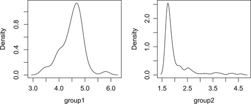It is not difficult to see the distribution of $y_i-{\mathbf{x}}_i^{\mathrm{\top }}{\hat{\mathit{\beta }}}^{\text{TS}}$ is multimodal. Consequently, it appears more appropriate to employ a model with heterogeneous intercepts to fit the dataset. Subsequently, in Figure 2, we present the density functions estimates of $y_i-{\mathbf{x}}_i^{\mathrm{\top }}{\hat{\mathit{\beta }}}^{\text{PS}}$ for two subgroups characterized by different intercepts, where ${\hat{\mathit{\beta }}}^{\text{PS}}$ is the coefficient vector estimate for proposed SCAD model. The density function estimates of the proposed MCP method exhibit similar characteristics and are therefore omitted here. When compared with the density functions shown in Figure 1, it is evident that each subgroup in Figure 2 displays an unimodal distribution with greater homogeneity.

Figure 1. Density plot of the response variable after adjusting for the effects of the covariates in the empirical example.

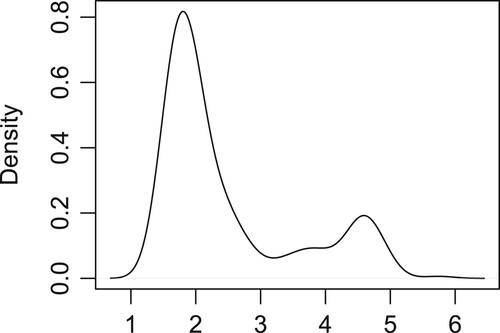
Figure 2. Density plots of response variable after adjusting for the effects of the covariates under two different intercept groups for proposed SCAD method.

The application of the proposed SCAD method leads to the detection of two subgroups with sample sizes of $n_1=47$ and $n_2=360$, respectively. It is worth noting that the patients in the OPTION design were originally categorized into two groups: a randomized group consisting of 356 patients, and a highly resistant group, comprising 51 patients. Consequently, we can consider this historical grouping as a control group structure. We calculate the rand index (RI) for the proposed SCAD method based on the control group structure. The rand index (RI) is 0.757, which indicates a substantial degree of agreement between the detected subgroup structure and the historical one. This suggests that the subgroup composition may undergo changes as a result of antiretroviral therapy, a phenomenon that is quite reasonable in the context of HIV patient management.

In addition, we compare the in-sample error and out-of-sample error for the aforementioned methods and the Tobit SCAD method with known subgroup structures. These errors are defined as the mean square error of $(i)\text{err}(y_i,\widehat{y_i})=(y_i-\widehat{y_i}{)}^2,(\mathrm{ii})\text{err}(y_i,{\widehat{y_i}}^{-})=(y_i-{\widehat{y_i}}^{-}{)}^2,i=1,\dots ,n$across all samples, where ${\hat{y}}_i$ is the fitted response, and ${\hat{y}}_i^{-}$ is the predicted response using a 5-fold cross-validation approach. To ensure comparability, we employ stratified sampling to maintain a consistent left-censored ratio across each test set. Table 6 presents the two types of criteria. For both two types of error, the Tobit SCAD method, when applied with known subgroup structures, exhibits smaller errors compared to the homogeneous model. This result underscores the significance of capturing the inherent heterogeneity within the dataset, as it enables more effective modelling of the influential variables affecting the response. While the errors in the control group are slightly larger compared to the proposed methods, it is essential to consider that these discrepancies may stem from changes in drug resistance among patients during treatment. Moreover, the disparities with the control group could serve as a basis for further examination of specific patient cases. It is conceivable that the existence of distinct groups may be attributed to disparities in the treatment trajectories of patients or inherent physiological differences among individuals. In clinical terms, these findings suggest the potential for devising more precise and tailored management protocols for specific patient subgroups, improving the overall treatment efficacy.

Table 6. The in-sample error and out-of-sample error

Method	In-sample error	Out-of-sample error
Tobit SCAD	0.91	1.08
proposed(SCAD)	$\mathbf{0.18}$	$\mathbf{0.17}$
proposed(MCP)	0.21	0.23
control(SCAD)	0.34	0.38

7. Conclusion

This paper introduces a novel approach to analysing censored data with potential heterogeneity in intercept effects by combining the penalty Tobit likelihood function with a concave fusion penalty. The proposed method can automatically identify heterogeneous structures in intercept effects and conduct variable selection.

To address the optimization problem associated with the method, we propose an algorithm based on the generalized coordinate descent method and alternating direction method of multipliers. This algorithm simplifies the optimization problem and reduces computational costs by employing a quadratic optimization function instead of a complex nonlinear optimization problem. This choice ensures efficient computation, particularly in scenarios with high complexity, while still maintaining good properties for the estimator. Furthermore, we establish the oracle property of parameter estimators. It is shown that within the domain of the oracle solution, a local minimum point of the objective function can be consistent with the oracle solution, providing theoretical support for the correctness of the method. Our ADMM-GCD algorithm with SCAD or MCP performs well in both extensive simulation case studies and the application of real data.

The proposed method can also be extended to incorporate the fusion of coefficient terms. However, there are still challenges in applying this method to generalized linear models or survival models, and further research is needed to develop algorithms and establish theoretical properties in these models.

Acknowledgements

We are very grateful to the editor, managing editor and the referee for their comments that improved this article.

Disclosure statement

No potential conflict of interest was reported by the author(s).

Additional information

Funding

This work was supported by the National Natural Science Foundation of China (NSF) of China [grant numbers 12171450 and 71921001.

Appendix

A.1. Proof of Proposition 3.1

First, according to the definition of ${\mathit{\eta }}^{(t+1)}$, we have $L({\mathit{\alpha }}^{(t+1)},{\mathit{\delta }}^{(t+1)},{\gamma }^{(t+1)},{\mathit{\eta }}^{(t+1)},{\mathit{\phi }}^{(t)})\le L({\mathit{\alpha }}^{(t+1)},{\mathit{\delta }}^{(t+1)},{\gamma }^{(t+1)},\mathit{\eta },{\mathit{\phi }}^{(t)})$for any $\mathit{\eta }$. Define $f^{(t+1)}=\underset{{\mathbf{\Delta }\mathit{\alpha }}^{(t+1)}-\mathit{\eta }=0}{inf}\{L({\mathit{\alpha }}^{(t+1)},{\mathit{\delta }}^{(t+1)},{\gamma }^{(t+1)},\mathit{\eta },{\mathit{\phi }}^{(t)})\},$and then we have $L({\mathit{\alpha }}^{(t+1)},{\mathit{\delta }}^{(t+1)},{\gamma }^{(t+1)},{\mathit{\eta }}^{(t+1)},{\mathit{\phi }}^{(t)})\le f^{(t+1)}.$Let k be a non-negative integer, since ${\mathit{\phi }}^{(t+k-1)}={\mathit{\phi }}^{(t)}+\rho \sum _{i=1}^{k-1}({\mathbf{\Delta }\mathit{\alpha }}^{(t+i)}-{\mathit{\eta }}^{(t+i)})$, so we can obtain that $\begin{array}{rl}& L({\mathit{\alpha }}^{(t+k)},{\mathit{\delta }}^{(t+k)},{\gamma }^{(t+k)},{\mathit{\eta }}^{(t+k)},{\mathit{\phi }}^{(t+k-1)})\\ & ={\ell }_n({\mathit{\alpha }}^{(t+k)},{\mathit{\delta }}^{(t+k)},{\gamma }^{(t+k)})+\sum _{j=1}^p{P}_{{\lambda }_1}(|{\delta }_j^{(t+k)}|)+\sum _{i<j}{P}_{{\lambda }_2}(|{\eta }_{\mathrm{ij}}^{(t+k)}|)\\ & +{\mathit{\phi }}^{(t+k-1)T}({\mathbf{\Delta }\mathit{\alpha }}^{(t+k)}-{\mathit{\eta }}^{(t+k)})+\frac{\rho }{2}\Vert {\mathbf{\Delta }\mathit{\alpha }}^{(t+k)}-{\mathit{\eta }}^{(t+k)}{\Vert }_2^2\\ & =S({\mathit{\alpha }}^{(t+k)},{\mathit{\delta }}^{(t+k)},{\gamma }^{(t+k)},{\mathit{\eta }}^{(t+k)})+\frac{\rho }{2}\Vert {\mathbf{\Delta }\mathit{\alpha }}^{(t+k)}-{\mathit{\eta }}^{(t+k)}{\Vert }_2^2\\ & +[{\mathit{\phi }}^{(t)}+\rho \sum _{i=1}^{k-1}({\mathbf{\Delta }\mathit{\alpha }}^{(t+i)}-{\mathit{\eta }}^{(t+i)})]\times ({\mathbf{\Delta }\mathit{\alpha }}^{(t+k)}-{\mathit{\eta }}^{(t+k)})\\ & \le f^{(t+k)}.\end{array}$According to Yang and Zou (2013), we can infer that the GCD limit point $({\mathit{\alpha }}^{(t+1)},{\mathit{\delta }}^{(t+1)},{\gamma }^{(t+1)})$ is the coordinatewise minimum of $L(\mathit{\alpha },\mathit{\delta },\gamma ,{\mathit{\eta }}^{(t)},{\mathit{\phi }}^{(t)})$. Additionally, the objective function is convex with respect to $\mathit{\eta }$. Then according to Theorem 4.1 in Tseng (2001), the sequence $({\mathit{\alpha }}^{(t)},{\mathit{\delta }}^{(t)},{\gamma }^{(t)},{\mathit{\eta }}^{(t)})$ converges to a coordinatewise minimum point $({\mathit{\alpha }}^{\ast },{\mathit{\delta }}^{\ast },{\gamma }^{\ast },{\mathit{\eta }}^{\ast })$. Thus we have $\begin{array}{rl}{f}^{\ast }& =\underset{t\to \mathrm{\infty }}{lim}{f}^{(t+1)}=\underset{t\to \mathrm{\infty }}{lim}{f}^{(t+k)}\\ & =\underset{{\mathbf{\Delta }\mathit{\alpha }}^{\ast }-\mathit{\eta }=0}{inf}\{{\ell }_n({\mathit{\alpha }}^{\ast },{\mathit{\delta }}^{\ast },{\gamma }^{\ast })+\sum _{j=1}^p{P}_{{\lambda }_1}(|{\delta }_j^{\ast }|)+\sum _{i<j}{P}_{{\lambda }_2}(|{\eta }_{\mathrm{ij}}|)\},\end{array}$and for all $k\ge 0$ $\begin{array}{rl}{f}^{\ast }\ge & \underset{t\to \mathrm{\infty }}{lim}L({\mathit{\alpha }}^{(t+k)},{\mathit{\delta }}^{(t+k)},{\gamma }^{(t+k)},{\mathit{\eta }}^{(t+k)},{\mathit{\phi }}^{(t+k-1)})\\ & ={\ell }_n({\mathit{\alpha }}^{\ast },{\mathit{\delta }}^{\ast },{\gamma }^{\ast })+\sum _{j=1}^p{P}_{{\lambda }_1}(|{\delta }_j^{\ast }|)+\sum _{i<j}{P}_{{\lambda }_2}(|{\eta }_{\mathrm{ij}}^{\ast }|)+\underset{t\to \mathrm{\infty }}{lim}{\mathit{\phi }}^{(t)\mathrm{\top }}(\mathbf{\Delta }{\mathit{\alpha }}^{\mathbf{\ast }}-{\mathit{\eta }}^{\ast })\\ & +(k-\frac{1}{2})\rho \Vert \mathbf{\Delta }{\mathit{\alpha }}^{\mathbf{\ast }}-{\mathit{\eta }}^{\ast }{\Vert }_2^2.\end{array}$Therefore, $(k-\frac{1}{2})\rho \Vert \mathbf{\Delta }{\mathit{\alpha }}^{\mathbf{\ast }}-{\mathit{\eta }}^{\ast }{\Vert }_2^2\le \underset{{\mathbf{\Delta }\mathit{\alpha }}^{\ast }-\mathit{\eta }=0}{inf}\{\sum _{i<j}{P}_{{\lambda }_2}(|{\eta }_{\mathrm{ij}}|)\}-\sum _{i<j}{P}_{{\lambda }_2}(|{\eta }_{\mathrm{ij}}^{\ast }|)-\underset{t\to \mathrm{\infty }}{lim}{\mathit{\phi }}^{(t)\mathrm{\top }}(\mathbf{\Delta }{\mathit{\alpha }}^{\mathbf{\ast }}-{\mathit{\eta }}^{\ast }).$Since the above inequality holds for all $k\ge 0$, then $\underset{t\to \mathrm{\infty }}{lim}\Vert {\mathbf{r}}^{(t)}{\Vert }_2^2=\Vert \mathbf{\Delta }{\mathit{\alpha }}^{\mathbf{\ast }}-{\mathit{\eta }}^{\ast }{\Vert }_2^2=0$.

Moreover, since $({\mathit{\alpha }}^{(t+1)},{\mathit{\delta }}^{(t+1)},{\gamma }^{(t+1)})$ minimize $L(\mathit{\alpha }\mathbf{,}\mathit{\delta },\gamma ,{\mathit{\eta }}^{(t)},{\mathit{\phi }}^{(t)})$, by definition, we have that $\begin{array}{rl}& \mathrm{\partial }L({\mathit{\alpha }}^{(t+1)},{\mathit{\delta }}^{(t+1)},{\gamma }^{(t+1)},{\mathit{\eta }}^{(t)},{\mathit{\phi }}^{(t)})/\mathrm{\partial }\mathit{\alpha }\\ & =\mathrm{\partial S}({\mathit{\alpha }}^{(t+1)},{\mathit{\delta }}^{(t+1)},{\gamma }^{(t+1)},{\mathit{\eta }}^{(t)})/\mathrm{\partial }\mathit{\alpha }+{\mathbf{\Delta }}^{\mathrm{\top }}{\mathit{\phi }}^{(t)}+\rho {\mathbf{\Delta }}^{\mathrm{\top }}({\mathbf{\Delta }\mathit{\alpha }}^{(t+1)}-{\mathit{\eta }}^{(t)})\\ & =\mathrm{\partial S}({\mathit{\alpha }}^{(t+1)},{\mathit{\delta }}^{(t+1)},{\gamma }^{(t+1)},{\mathit{\eta }}^{(t)})/\mathrm{\partial }\mathit{\alpha }+{\mathbf{\Delta }}^{\mathrm{\top }}({\mathit{\phi }}^{(t)}+\rho ({\mathbf{\Delta }\mathit{\alpha }}^{(t+1)}-{\mathit{\eta }}^{(t)}))\\ & =\mathrm{\partial S}({\mathit{\alpha }}^{(t+1)},{\mathit{\delta }}^{(t+1)},{\gamma }^{(t+1)},{\mathit{\eta }}^{(t)})/\mathrm{\partial }\mathit{\alpha }+{\mathbf{\Delta }}^{\mathrm{\top }}{\mathit{\phi }}^{(t+1)}+\rho {\mathbf{\Delta }}^{\mathrm{\top }}({\mathit{\eta }}^{(t+1)}-{\mathit{\eta }}^{(t)})=0.\end{array}$Thus, $\Vert {\mathbf{s}}^{(t+1)}{\Vert }_2^2=\rho {\mathbf{\Delta }}^{\mathrm{\top }}({\mathit{\eta }}^{(t+1)}-{\mathit{\eta }}^{(t)})=-(\mathrm{\partial S}({\mathit{\alpha }}^{(t+1)},{\mathit{\delta }}^{(t+1)},{\gamma }^{(t+1)},{\mathit{\eta }}^{(t)})/\mathrm{\partial }\mathit{\alpha }+{\mathbf{\Delta }}^{\mathrm{\top }}{\mathit{\phi }}^{(t+1)})$ Since $\underset{t\to \mathrm{\infty }}{lim}\Vert {\mathbf{r}}^{(t)}{\Vert }_2^2=\Vert \mathbf{\Delta }{\mathit{\alpha }}^{\mathbf{\ast }}-{\mathit{\eta }}^{\ast }{\Vert }_2^2=0$, $\begin{array}{rl}& \underset{t\to \mathrm{\infty }}{lim}\mathrm{\partial L}({\mathit{\alpha }}^{(t+1)},{\mathit{\delta }}^{(t+1)},{\gamma }^{(t+1)},{\mathit{\eta }}^{(t)},{\mathit{\phi }}^{(t)})/\mathrm{\partial }\mathit{\alpha }\\ & =\underset{t\to \mathrm{\infty }}{lim}\mathrm{\partial S}({\mathit{\alpha }}^{(t+1)},{\mathit{\delta }}^{(t+1)},{\gamma }^{(t+1)},{\mathit{\eta }}^{(t)})/\mathrm{\partial }\mathit{\alpha }+{\mathbf{\Delta }}^{\mathrm{\top }}{\mathit{\phi }}^{(t)}=0.\end{array}$Therefore, $\underset{t\to \mathrm{\infty }}{lim}\Vert {\mathbf{s}}^{(t+1)}{\Vert }_2^2=0$.

A.2. Proof of Theorem 4.1

Let $\mathit{\theta }=({\hat{\mathrm{\Xi }}}^{(\mathrm{or})}-{\hat{\mathrm{\Xi }}}^{\ast })$, q = K + s + 1. We can see that $\sqrt{n}\mathit{\theta }\sim N(0,\mathbf{\Sigma })$ according to (20(20) $\begin{array}{r}\sqrt{n}({\hat{\mathrm{\Xi }}}^{\text{or}}-{\mathrm{\Xi }}^{\ast })\to N(\mathbf{0},\mathbf{\Sigma }),\end{array}$(20) ) where $\mathbf{\Sigma }=[-\frac{1}{n}{\mathrm{\nabla }}^2\log L_n(\mathrm{\Xi }){|}_{\mathrm{\Xi }={\mathrm{\Xi }}^{\ast }}{]}^{-1}$.

In order to get the tail probability of the event in (21(21) $\begin{array}{r}{\Vert {\hat{\mathrm{\Theta }}}^{\mathrm{or}}-{\mathrm{\Theta }}^{\ast }\Vert }_{\mathrm{\infty }}\le {\varphi }_n,\end{array}$(21) ), we introduce a q-dimension vector $\mathbf{a}=(a_1,\dots ,a_q{)}^{\mathrm{\top }}$ satisfying $\Vert \mathbf{a}{\Vert }_2=1$, that is $a_1^2+\dots +a_q^2=1$. It is obvious that ${\mathbf{a}}^{\mathrm{\top }}\mathit{\theta }\sim N(0,\frac{1}{n}{\mathbf{a}}^{\mathrm{\top }}\mathbf{\Sigma }\mathbf{a})$. Since $|{\mathbf{a}}^{\mathrm{\top }}\mathit{\theta }|=|a_1{\theta }_1+\dots +a_q{\theta }_q|\le |a_1{\theta }_1|+\dots +|a_q{\theta }_q|,$$|{\mathbf{a}}^{\mathrm{\top }}\mathit{\theta }|\le 1\cdot |{\theta }_j{|}_{max}$. Then it is easy to get $\underset{\Vert \mathbf{a}{\Vert }_2=1}{max}|{\mathbf{a}}^{\mathrm{\top }}\mathit{\theta }|=\underset{j}{max}|{\theta }_j|$. Since $\mathbf{\Sigma }$ is a symmetric positive definite matrix, the maximum value of the quadratic $f={\mathbf{a}}^{\mathrm{\top }}\mathbf{\Sigma }\mathbf{a}$ at $\Vert \mathbf{a}\Vert =1$ is the largest eigenvalue ${\lambda }_{max}$ of the matrix $\mathbf{\Sigma }$.

For a normal distribution $X\sim N(0,{\sigma }^2)$, the two-tailed probability inequality is (A1) $\begin{array}{r}P(|X|<c)\ge 1-\sqrt{\frac{2}{\pi }}\cdot \frac{\sigma }{c}\cdot \exp \{-\frac{c^2}{2{\sigma }^2}\}.\end{array}$(A1) So $P(|{\mathbf{a}}^{\mathrm{\top }}\mathit{\theta }|<{\varphi }_n)\ge 1-\sqrt{\frac{2}{\pi }}\cdot \frac{\sqrt{f/n}}{{\varphi }_n}\cdot \exp \{-\frac{{\varphi }_n^2}{2(f/n)}\}.$Since the right-side of the above inequality with respect to f is a decreasing function, then $P(\underset{\Vert \mathbf{a}{\Vert }_2=1}{max}|{\mathbf{a}}^{\mathrm{\top }}\mathit{\theta }|<{\varphi }_n)\ge 1-\sqrt{\frac{2}{\pi }}\cdot \frac{\sqrt{{\lambda }_{max}/n}}{{\varphi }_n}\cdot \exp \{-\frac{{\varphi }_n^2}{2({\lambda }_{max}/n)}\}.$Therefore, (A2) $\begin{array}{rl}& P({\Vert {\hat{\mathrm{\Theta }}}^{\text{or}}-{\mathrm{\Theta }}^{\ast }\Vert }_{\mathrm{\infty }}<{\varphi }_n)=P({\Vert {\hat{\mathrm{\Xi }}}^{\text{or}}-{\mathrm{\Xi }}^{\ast }\Vert }_{\mathrm{\infty }}<{\varphi }_n)\\ & =P(\underset{j}{max}|{\theta }_j|<{\varphi }_n)=P(\underset{\Vert \mathbf{a}{\Vert }_2=1}{max}|{\mathbf{a}}^{\mathrm{\top }}\mathit{\theta }|<{\varphi }_n)\\ & \ge 1-\sqrt{\frac{2}{\pi }}\cdot \frac{\sqrt{{\lambda }_{max}/n}}{{\varphi }_n}\cdot \exp \{-\frac{{\varphi }_n^2}{2({\lambda }_{max}/n)}\}.\end{array}$(A2) Since ${\lambda }_{max}=O(1)$, we set ${\varphi }_n=1/\sqrt{\log n}$ and $t=\sqrt{\log n/n}$. Then $P(\Vert {\hat{\mathrm{\Theta }}}^{\text{or}}-{\mathrm{\Theta }}^{\ast }{\Vert }_{\mathrm{\infty }}<{\varphi }_n)\ge 1-C\sqrt{\frac{\log n}{n}}\cdot \exp \{-\frac{n}{2\log n}\}=1-C\cdot \mathrm{texp}\{-\frac{1}{2t^2}\}$, where C is a constant. Obviously we have $t\to 0$ and then $P(\Vert {\hat{\mathrm{\Theta }}}^{\text{or}}-{\mathrm{\Theta }}^{\ast }{\Vert }_{\mathrm{\infty }}<{\varphi }_n)\to 1$ when $n\to \mathrm{\infty }$.

A.3. Proof of Theorem 4.2

First, with the underlying group division ${\mathcal{G}}_1,\dots ,{\mathcal{G}}_K$ and true support set $\mathcal{A}$ we define $\begin{array}{rl}{L}_n(\mathit{\alpha },\mathit{\delta },\gamma )& ={\ell }_n(\mathit{\alpha },\mathit{\delta },\gamma ),P_{{\lambda }_1}(\mathit{\delta })={\lambda }_1\sum _{j=1}^p\rho (|{\delta }_j|),P_{{\lambda }_2}(\mathit{\alpha })={\lambda }_2\sum _{i<j}\rho (|{\alpha }_i-{\alpha }_j|),\\ L_n^{\mathcal{O}}(\mathit{\tau },{\mathit{\delta }}_{\mathbf{1}},\gamma )& ={\ell }_n^{\mathcal{O}}(\mathit{\tau },{\mathit{\delta }}_{\mathbf{1}},\gamma ),P_{{\lambda }_1}^{\mathcal{O}}({\mathit{\delta }}_{\mathbf{1}})={\lambda }_1\sum _{j\in \mathcal{A}}\rho (|{\delta }_j|),P_{{\lambda }_2}^{\mathcal{O}}(\mathit{\tau })={\lambda }_2\sum _{k<k^{\prime }}|{\mathcal{G}}_k||{\mathcal{G}}_{k^{\prime }}|\rho (|{\tau }_i-{\tau }_j|),\end{array}$and denote $\begin{array}{rl}& Q_n(\mathit{\alpha },\mathit{\delta },\gamma )=L_n(\mathit{\alpha }\mathbf{,}\mathit{\delta },\gamma )+P_{{\lambda }_1}(\mathit{\delta })+P_{{\lambda }_2}(\mathit{\alpha }),\\ & Q_n^{\mathcal{O}}(\mathit{\tau },{\mathit{\delta }}_{\mathbf{1}},\gamma )=L_n^{\mathcal{O}}(\mathit{\tau },{\mathit{\delta }}_{\mathbf{1}},\gamma )+P_{{\lambda }_1}^{\mathcal{O}}({\mathit{\delta }}_{\mathbf{1}})+P_{{\lambda }_2}^{\mathcal{O}}(\mathit{\tau }).\end{array}$Let $T:{\mathcal{M}}_{\mathcal{G}}\to R^K$ be the mapping such as that $T(\mathit{\alpha })$ is the $K\times 1$ vector whose kth coordinate equals to the common value of ${\alpha }_i$ for $i\in {\mathcal{G}}_k$. And let $T_0:R^n\to R^K$ be the mapping such that $T_0(\mathit{\alpha })=\{|{\mathcal{G}}_k{|}^{-1}\sum _{i\in {\mathcal{G}}_k}{\alpha }_i{\}}_{k=1}^K$. Let $S:R^p\to R^s$ be the mapping such that $S(\mathit{\delta })$ retains only the part of $\mathit{\delta }$ whose corner is labelled $\mathcal{A}$, that is $S(\mathit{\delta })={\mathit{\delta }}_{\mathcal{A}}$. And let $S^{-1}:R^s\to {\mathcal{M}}_{\mathcal{B}}$ be the mapping such that $S^{-1}({\mathit{\delta }}_{\mathbf{1}})=({\mathit{\delta }}_{\mathbf{1}}^{\mathrm{\top }},{\mathbf{0}}_{{\mathcal{A}}^c}^{\mathrm{\top }}{)}^{\mathrm{\top }}$. Obviously, when $\mathit{\alpha }\in {\mathcal{M}}_{\mathcal{G}}$ and $\mathit{\delta }\in {\mathcal{M}}_{\mathcal{B}}$, $T(\mathit{\alpha })=T_0(\mathit{\alpha })$ and ${\mathit{\delta }}_{\mathcal{A}}=S(\mathit{\delta })$. Moreover, for every $\mathit{\delta }\in {\mathcal{M}}_{\mathcal{B}}$ and $\mathit{\alpha }\in {\mathcal{M}}_{\mathcal{G}}$, we have $P_{{\lambda }_1}(\mathit{\delta })=P_{{\lambda }_1}^{\mathcal{O}}({\mathit{\delta }}_{\mathcal{A}})$ and $P_{{\lambda }_2}(\mathit{\alpha })=P_{{\lambda }_2}^{\mathcal{O}}(T(\mathit{\alpha }))$. For every ${\mathit{\delta }}_{\mathbf{1}}\in R^s$ and $\mathit{\tau }\in R^K$, we have $P_{{\lambda }_1}(S^{-1}({\mathit{\delta }}_{\mathbf{1}}))=P_{{\lambda }_1}^{\mathcal{O}}({\mathit{\delta }}_{\mathbf{1}})$ and $P_{{\lambda }_2}(T^{-1}(\mathit{\tau }))=P_{{\lambda }_2}^{\mathcal{O}}(\mathit{\tau })$. Hence (A3) $\begin{array}{r}{Q}_n(\mathit{\alpha },\mathit{\delta },\gamma )=Q_n^{\mathcal{O}}(T(\mathit{\alpha }),{\mathit{\delta }}_{\mathcal{A}},\gamma ),Q_n^{\mathcal{O}}(\mathit{\tau },{\mathit{\delta }}_{\mathbf{1}},\gamma )=Q_n(T^{-1}(\mathit{\tau }),S^{-1}({\mathit{\delta }}_{\mathbf{1}}),\gamma ).\end{array}$(A3) Consider the neighbourhood of $({\mathit{\alpha }}^{\mathbf{\ast }},{\mathit{\delta }}^{\mathbf{\ast }},{\gamma }^{\ast })$ $\mathrm{\Psi }=\{\mathit{\alpha }\in R^n,\mathit{\delta }\in R^p,\gamma \in R:{\Vert ((\mathit{\alpha }\mathbf{-}{\mathit{\alpha }}^{\mathbf{\ast }}{)}^{\mathrm{\top }},(\mathit{\delta }\mathbf{-}{\mathit{\delta }}^{\mathbf{\ast }}{)}^{\mathrm{\top }},\gamma -{\gamma }^{\ast }{)}^{\mathrm{\top }}\Vert }_{\mathrm{\infty }}\le {\varphi }_n\}.$Define the event $E_1=\{\hat{\mathrm{\Theta }}\in \mathrm{\Psi }\}$. By Theorem 1 we have $P(E_1^c)\le p_1$. For any $\mathit{\alpha }\in R^n$ and $\mathit{\delta }\in R^p$ let ${\mathit{\alpha }}^{\mathbf{0}}=T^{-1}(T_0(\mathit{\alpha }))$ and ${\mathit{\delta }}^{\mathbf{0}}=S^{-1}({\mathit{\delta }}_{\mathcal{A}})$. We will prove that $({\hat{\mathit{\alpha }}}^{\text{or}},{\hat{\mathit{\delta }}}^{\text{or}},{\hat{\gamma }}^{\text{or}})$ is a local minimizer of the objective function $Q_n(\mathit{\alpha },\mathit{\delta },\gamma )$ with probability approaching 1 through the following two steps.

1. On the event $E_1$, $Q_n({\mathit{\alpha }}^{\mathbf{0}},{\mathit{\delta }}^{\mathbf{0}},\gamma )\ge Q_n({\hat{\mathit{\alpha }}}^{\text{or}},{\hat{\mathit{\delta }}}^{\text{or}},{\hat{\gamma }}^{\text{or}})$ for any $({\mathit{\alpha }}^{\mathrm{\top }},{\mathit{\delta }}^{\mathrm{\top }},\gamma {)}^{\mathrm{\top }}\in \mathrm{\Psi }$.

2. There is an event $E_2$ such that $P(E_2^c)\le p_2=\frac{n_1}{n\sqrt{\log n}}$. On $E_1\cap E_2$, there is a neighbourhood of $(({\hat{\mathit{\alpha }}}^{\text{or}}{)}^{\mathrm{\top }},({\hat{\mathit{\delta }}}^{\text{or}}{)}^{\mathrm{\top }},{\hat{\gamma }}^{\text{or}}{)}^{\mathrm{\top }}$, denoted by ${\mathrm{\Psi }}_n=\{\mathit{\alpha },\mathit{\delta }:\Vert ((\mathit{\alpha }-{\hat{\mathit{\alpha }}}^{\text{or}}{)}^{\mathrm{\top }},(\mathit{\delta }-{\hat{\mathit{\delta }}}^{\text{or}}{)}^{\mathrm{\top }}{)}^{\mathrm{\top }}{\Vert }_{\mathrm{\infty }}\le t_n\}$ such that $Q_n(\mathit{\alpha },\mathit{\delta },\gamma )\ge Q_n({\mathit{\alpha }}^{\mathbf{0}},{\mathit{\delta }}^{\mathbf{0}},\gamma )$ for any $({\mathit{\alpha }}^{\mathrm{\top }},{\mathit{\delta }}^{\mathrm{\top }},\gamma {)}^{\mathrm{\top }}\in \mathrm{\Psi }\cap {\mathrm{\Psi }}_n$ for sufficiently large n.

Therefore, by the result of (i) and (ii), we have $Q_n(\mathit{\alpha },\mathit{\delta },\gamma )\ge Q_n({\hat{\mathit{\alpha }}}^{\text{or}},{\hat{\mathit{\delta }}}^{\text{or}},{\hat{\gamma }}^{\text{or}})$ for any $({\mathit{\alpha }}^{\mathrm{\top }},{\mathit{\delta }}^{\mathrm{\top }},\gamma {)}^{\mathrm{\top }}\in \mathrm{\Psi }\cap {\mathrm{\Psi }}_n$, so that $(({\hat{\mathit{\alpha }}}^{\text{or}}{)}^{\mathrm{\top }},({\hat{\mathit{\delta }}}^{\text{or}}{)}^{\mathrm{\top }},{\hat{\gamma }}^{\text{or}}{)}^{\mathrm{\top }}$ is a strict local minimizer of $Q_n(\mathit{\alpha },\mathit{\delta },\gamma )$ on the event $E_1\cap E_2$ with $P(E_1\cap E_2)\ge 1-p_1-p_2$ for sufficiently large n.

Step (i): Since $({\hat{\mathit{\tau }}}^{\text{or}},{\hat{\mathit{\delta }}}_1^{\text{or}},{\hat{\gamma }}^{\text{or}})$ is a global minimizer of $L_n^{\mathcal{O}}(\mathit{\tau },{\mathit{\delta }}_{\mathbf{1}},\gamma )$, $L_n^{\mathcal{O}}(T_0(\mathit{\alpha }),S(\mathit{\delta }),\gamma )\ge L_n^{\mathcal{O}}({\hat{\mathit{\tau }}}^{\mathrm{or}},{\hat{\mathit{\delta }}}_1^{\mathrm{or}},{\hat{\gamma }}^{\mathrm{or}})$ for all $({\mathit{\alpha }}^{\mathrm{\top }},{\mathit{\delta }}^{\mathrm{\top }},\gamma )\in \mathrm{\Psi }$. Then we derive that $P_{{\lambda }_1}^{\mathcal{O}}(S(\mathit{\delta }))$ is a constant which does not depend on $\mathit{\delta }$ for $\mathit{\delta }\in \mathrm{\Psi }$ and $P_{{\lambda }_2}^{\mathcal{O}}(T_0(\mathit{\alpha }))$ is also a constant which does not depend on $\mathit{\alpha }$ for $\mathit{\alpha }\in \mathrm{\Psi }$. Let $T_0(\mathit{\alpha })=\mathit{\tau }=({\tau }_1,\dots ,{\tau }_K{)}^{\mathrm{\top }}$. For any $k\ne k^{\prime }$, since $\begin{array}{rl}|{\tau }_k^{\ast }-{\tau }_{k^{\prime }}^{\ast }|& =|{\tau }_k^{\ast }-{\tau }_{k^{\prime }}^{\ast }+{\tau }_k-{\tau }_k+{\tau }_{k^{\prime }}-{\tau }_{k^{\prime }}|\\ & \le |{\tau }_k-{\tau }_{k^{\prime }}|+|{\tau }_k^{\ast }-{\tau }_k|+|{\tau }_{k^{\prime }}-{\tau }_{k^{\prime }}^{\ast }|,\end{array}$so $|{\tau }_k-{\tau }_{k^{\prime }}|\ge |{\tau }_k^{\ast }-{\tau }_{k^{\prime }}^{\ast }|-2\underset{k}{sup}|{\tau }_k-{\tau }_k^{\ast }|,$and (A4) $\begin{array}{rl}\underset{k}{sup}|{\tau }_k-{\tau }_k^{\ast }|& =\underset{k}{sup}|\sum _{i\in {\mathcal{G}}_k}{\alpha }_i/|{\mathcal{G}}_k|-{\tau }_k^{\ast }|=\underset{k}{sup}|\sum _{i\in {\mathcal{G}}_k}({\alpha }_i-{\alpha }_k^{\ast })/|{\mathcal{G}}_k||\\ & \le \underset{k}{sup}\underset{i\in {\mathcal{G}}_k}{sup}|{\alpha }_i-{\alpha }_i^{\ast }|=\Vert \mathit{\alpha }\mathbf{-}{\mathit{\alpha }}^{\mathbf{\ast }}{\Vert }_{\mathrm{\infty }}.\end{array}$(A4) Therefore, for all k and $k^{\prime }$, $|{\tau }_k-{\tau }_{k^{\prime }}|\ge |{\tau }_k^{\ast }-{\tau }_{k^{\prime }}^{\ast }|-2\Vert {\alpha }_k-{\alpha }_k^{\ast }{\Vert }_{\mathrm{\infty }}\ge b_n-2{\varphi }_n>a{\lambda }_2,$which indicates $\rho (|{\tau }_k-{\tau }_{k^{\prime }}|)$ is a constant by Condition (C2), and as a result $P_{{\lambda }_2}^{\mathcal{G}}(T_0(\mathit{\alpha }))$ is also a constant. Similarly, for any $j\in \mathcal{A}$, let $S(\mathit{\alpha })={\mathit{\delta }}_{\mathbf{1}}=({\delta }_1,\dots ,{\delta }_{p_1})$, since $|{\delta }_j^{\ast }|=|{\delta }_j^{\ast }-{\delta }_j+{\delta }_j|\le |{\delta }_j^{\ast }-{\delta }_j|+|{\delta }_j|$By the condition $|{\mathit{\delta }}_{\mathcal{A}}{|}_{min}>(a+1){\lambda }_1$, we have $|{\delta }_j|\ge \Vert {\mathit{\delta }}^{\ast }{\Vert }_{min}-\Vert {\mathit{\delta }}^{\ast }-\mathit{\delta }{\Vert }_{\mathrm{\infty }}\ge \Vert {\mathit{\delta }}^{\ast }{\Vert }_{min}-\Vert {\mathrm{\Theta }}^{\ast }-\mathrm{\Theta }{\Vert }_{\mathrm{\infty }}\ge (a+1){\lambda }_1-{\varphi }_n\ge a{\lambda }_1.$As a result, both $\rho (|{\delta }_j|)$ and $P_{{\lambda }_1}^{\mathcal{O}}(S(\mathit{\delta }))$ are constants.

On conclusion, we have $Q_n^{\mathcal{O}}(T_0(\mathit{\alpha }),S(\mathit{\delta }),\gamma )\ge Q_n^{\mathcal{O}}({\hat{\mathit{\tau }}}^{\text{or}},{\hat{\mathit{\delta }}}_1^{\text{or}},{\hat{\gamma }}^{\text{or}})$ for all $({\mathit{\alpha }}^{\mathrm{\top }},{\mathit{\delta }}^{\mathrm{\top }},\gamma )\in \mathrm{\Psi }$. In addition, $Q_n^{\mathcal{O}}({\hat{\mathit{\tau }}}^{\text{or}},{\hat{\mathit{\delta }}}_1^{\text{or}},{\hat{\gamma }}^{\mathrm{or}})=Q_n({\hat{\mathit{\alpha }}}^{\text{or}},{\hat{\mathit{\delta }}}^{\text{or}},{\hat{\gamma }}^{\text{or}})$ and $Q_n^{\mathcal{O}}(T_0(\mathit{\alpha }),S(\mathit{\delta }),\gamma )=Q_n(T^{-1}(T_0(\mathit{\alpha })),S^{-1}({\mathit{\delta }}_{\mathcal{A}}),\gamma )=Q_n({\mathit{\alpha }}^{\mathbf{0}},{\mathit{\delta }}^{\mathbf{0}},\gamma )$. Hence, we get $Q_n({\mathit{\alpha }}^{\mathbf{0}},{\mathit{\delta }}^{\mathbf{0}},\gamma )\ge Q_n({\hat{\mathit{\alpha }}}^{\text{or}},{\hat{\mathit{\delta }}}^{\text{or}},{\hat{\gamma }}^{\text{or}})$, and the result in (i) is proved.

Step (ii): First, we introduce a neighbourhood ${\mathrm{\Psi }}_n=\{\mathit{\alpha },\mathit{\delta }:\Vert ((\mathit{\alpha }-{\hat{\mathit{\alpha }}}^{\text{or}}{)}^{\mathrm{\top }},(\mathit{\delta }-{\hat{\mathit{\delta }}}^{\text{or}}{)}^{\mathrm{\top }}{)}^{\mathrm{\top }}{\Vert }_{\mathrm{\infty }}\le t_n\}$ for a positive sequence $t_n$. For $({\mathit{\alpha }}^{\mathrm{\top }},{\mathit{\delta }}^{\mathrm{\top }},\gamma )\in \mathrm{\Psi }\cap {\mathrm{\Psi }}_n$, by Taylor's expansion at $({\mathit{\alpha }}^0,{\mathit{\delta }}^{\mathbf{0}})$, we have $\begin{array}{rl}& Q_n(\mathit{\alpha },\mathit{\delta },\gamma )-Q_n({\mathit{\alpha }}^{\mathbf{0}},{\mathit{\delta }}^{\mathbf{0}},\gamma )\\ & =-\mathbf{w}(\mathit{\alpha }\mathbf{-}{\mathit{\alpha }}^{\mathbf{0}})+\sum _{i=1}^n\frac{\mathrm{\partial }{P}_{{\lambda }_2}({\mathit{\alpha }}^m)}{\mathrm{\partial }{\alpha }_i}({\alpha }_i-{\alpha }_i^0)-\mathbf{v}(\mathit{\delta }-{\mathit{\delta }}^{\mathbf{0}})+\sum _{j=1}^p\frac{\mathrm{\partial }{P}_{{\lambda }_1}({\mathit{\delta }}^m)}{\mathrm{\partial }{\delta }_j}({\delta }_j-{\delta }_j^0)\\ & ={\mathrm{\Gamma }}_1+{\mathrm{\Gamma }}_2+{\mathrm{\Gamma }}_3+{\mathrm{\Gamma }}_4,\end{array}$where $\mathbf{w}=[\frac{1}{n_1}(\gamma {\mathbf{y}}_1-{\mathit{\alpha }}_1^m-{\mathbf{X}}_1\mathit{\delta }{)}^{\mathrm{\top }},-\frac{1}{n_0}g(-{\mathit{\alpha }}_0^m-{\mathbf{X}}_0\mathit{\delta }{)}^{\mathrm{\top }}{]}^{\mathrm{\top }}=(\frac{1}{n_1}{\mathrm{\Lambda }}_1^{\mathrm{\top }},-\frac{1}{n_0}{\mathrm{\Lambda }}_2^{\mathrm{\top }}{)}^{\mathrm{\top }}$ and $\mathbf{v}=\frac{1}{n_1}{\mathbf{X}}_1^{\mathrm{\top }}(\gamma {\mathbf{y}}_1-{\mathit{\alpha }}_1^m-{\mathbf{X}}_1{\mathit{\delta }}^m)-\frac{1}{n_0}{\mathbf{X}}_0^{\mathrm{\top }}g(-{\mathit{\alpha }}_0^m-{\mathbf{X}}_0^{\mathrm{\top }}{\mathit{\delta }}^m)=\frac{1}{n_1}{\mathbf{X}}_1^{\mathrm{\top }}{\mathrm{\Lambda }}_1+\frac{1}{n_0}{\mathbf{X}}_0^{\mathrm{\top }}{\mathrm{\Lambda }}_2$ in which ${\mathit{\alpha }}^m={\zeta }_1\mathit{\alpha }+(1-{\zeta }_1){\mathit{\alpha }}^{\mathbf{0}}$ and ${\mathit{\delta }}^m={\zeta }_2\mathit{\delta }+(1-{\zeta }_2){\mathit{\delta }}^{\mathbf{0}}$ for some ${\zeta }_1,{\zeta }_2\in (0,1)$. Firstly, (A5) $\begin{array}{rl}{\mathrm{\Gamma }}_1& =-{\mathbf{w}}^{\mathrm{\top }}(\mathit{\alpha }\mathbf{-}{\mathit{\alpha }}^{\mathbf{0}})=-\sum _{k=1}^K\sum _{\{i,j\in {\mathcal{G}}_k\}}\frac{w_i({\alpha }_i-{\alpha }_j)}{|{\mathcal{G}}_k|}\\ & =-\sum _{k=1}^K\sum _{\{i,j\in {\mathcal{G}}_k\}}\frac{w_i({\alpha }_i-{\alpha }_j)}{2|{\mathcal{G}}_k|}-\sum _{k=1}^K\sum _{i,j\in {\mathcal{G}}_k}\frac{w_i({\alpha }_i-{\alpha }_j)}{2|{\mathcal{G}}_k|}\\ & =-\sum _{k=1}^K\sum _{\{i,j\in {\mathcal{G}}_k\}}\frac{(w_j-w_i)({\alpha }_j-{\alpha }_i)}{2|{\mathcal{G}}_k|}\\ & =-\sum _{k=1}^K\sum _{\{i,j\in {\mathcal{G}}_k,i<j\}}\frac{(w_j-w_i)({\alpha }_j-{\alpha }_i)}{|{\mathcal{G}}_k|}.\end{array}$(A5) As shown in (A4(A4) $\begin{array}{rl}\underset{k}{sup}|{\tau }_k-{\tau }_k^{\ast }|& =\underset{k}{sup}|\sum _{i\in {\mathcal{G}}_k}{\alpha }_i/|{\mathcal{G}}_k|-{\tau }_k^{\ast }|=\underset{k}{sup}|\sum _{i\in {\mathcal{G}}_k}({\alpha }_i-{\alpha }_k^{\ast })/|{\mathcal{G}}_k||\\ & \le \underset{k}{sup}\underset{i\in {\mathcal{G}}_k}{sup}|{\alpha }_i-{\alpha }_i^{\ast }|=\Vert \mathit{\alpha }\mathbf{-}{\mathit{\alpha }}^{\mathbf{\ast }}{\Vert }_{\mathrm{\infty }}.\end{array}$(A4) ), (A6) $\begin{array}{r}\Vert {\mathit{\alpha }}^0-{\mathit{\alpha }}^{\ast }{\Vert }_{\mathrm{\infty }}=\Vert \mathit{\tau }\mathbf{-}{\mathit{\tau }}^{\mathbf{\ast }}{\Vert }_{\mathrm{\infty }}\le \Vert \mathit{\alpha }\mathbf{-}{\mathit{\alpha }}^{\mathbf{\ast }}{\Vert }_{\mathrm{\infty }}.\end{array}$(A6) Since ${\mathit{\alpha }}^m={\zeta }_1\mathit{\alpha }+(1-{\zeta }_1){\mathit{\alpha }}^0$, (A7) $\begin{array}{r}\Vert {\mathit{\alpha }}^m-{\mathit{\alpha }}^{\ast }{\Vert }_{\mathrm{\infty }}\le \Vert \mathit{\alpha }\mathbf{-}{\mathit{\alpha }}^{\mathbf{\ast }}{\Vert }_{\mathrm{\infty }}\le {\varphi }_n.\end{array}$(A7) As the same steps in (A4(A4) $\begin{array}{rl}\underset{k}{sup}|{\tau }_k-{\tau }_k^{\ast }|& =\underset{k}{sup}|\sum _{i\in {\mathcal{G}}_k}{\alpha }_i/|{\mathcal{G}}_k|-{\tau }_k^{\ast }|=\underset{k}{sup}|\sum _{i\in {\mathcal{G}}_k}({\alpha }_i-{\alpha }_k^{\ast })/|{\mathcal{G}}_k||\\ & \le \underset{k}{sup}\underset{i\in {\mathcal{G}}_k}{sup}|{\alpha }_i-{\alpha }_i^{\ast }|=\Vert \mathit{\alpha }\mathbf{-}{\mathit{\alpha }}^{\mathbf{\ast }}{\Vert }_{\mathrm{\infty }}.\end{array}$(A4) ) and (A6(A6) $\begin{array}{r}\Vert {\mathit{\alpha }}^0-{\mathit{\alpha }}^{\ast }{\Vert }_{\mathrm{\infty }}=\Vert \mathit{\tau }\mathbf{-}{\mathit{\tau }}^{\mathbf{\ast }}{\Vert }_{\mathrm{\infty }}\le \Vert \mathit{\alpha }\mathbf{-}{\mathit{\alpha }}^{\mathbf{\ast }}{\Vert }_{\mathrm{\infty }}.\end{array}$(A6) ), (A8) $\begin{array}{r}\Vert {\mathit{\delta }}^{\mathbf{0}}-{\mathit{\delta }}^{\ast }{\Vert }_{\mathrm{\infty }}=\Vert {\mathit{\delta }}_{\mathbf{1}}-{\mathit{\delta }}_{\mathbf{1}}^{\ast }{\Vert }_{\mathrm{\infty }}\le \Vert \mathit{\delta }-{\mathit{\delta }}^{\ast }{\Vert }_{\mathrm{\infty }}.\end{array}$(A8) Since ${\mathit{\delta }}^m={\zeta }_2\mathit{\delta }+(1-{\zeta }_2){\mathit{\delta }}^{\mathbf{0}}$, (A9) $\begin{array}{r}\Vert {\mathit{\delta }}^m-{\mathit{\delta }}^{\ast }{\Vert }_{\mathrm{\infty }}\le \Vert \mathit{\delta }-{\mathit{\delta }}^{\ast }{\Vert }_{\mathrm{\infty }}\le {\varphi }_n.\end{array}$(A9) Then by Condition (C1), $\begin{array}{rl}{\mathrm{\Lambda }}_1& =\frac{\gamma }{{\gamma }^{\ast }}({\mathit{\alpha }}_1^{\ast }+{\mathbf{X}}_1{\mathit{\delta }}^{\ast }+{\mathit{\epsilon }}_1{\gamma }^{\ast })-{\mathbf{X}}_1{\mathit{\delta }}^m-{\mathit{\alpha }}_1^m\\ & =\frac{\gamma -{\gamma }^{\ast }}{{\gamma }^{\ast }}({\mathit{\alpha }}_1^{\ast }+{\mathbf{X}}_1{\mathit{\delta }}^{\ast })+{\mathit{\alpha }}_1^{\ast }-{\mathit{\alpha }}_1^m+{\mathbf{X}}_1({\mathit{\delta }}^{\ast }-{\mathit{\delta }}^m)+(\gamma -{\gamma }^{\ast }+{\gamma }^{\ast }){\mathit{\epsilon }}_1,\\ \Vert {\mathrm{\Lambda }}_1{\Vert }_{\mathrm{\infty }}& \le \frac{\Vert \gamma -{\gamma }^{\ast }{\Vert }_{\mathrm{\infty }}}{\Vert {\gamma }^{\ast }{\Vert }_{\mathrm{\infty }}}(\Vert {\mathit{\alpha }}_1^{\ast }{\Vert }_{\mathrm{\infty }}+\Vert {\mathbf{X}}_1{\mathit{\delta }}^{\ast }{\Vert }_{\mathrm{\infty }})+\Vert {\mathit{\alpha }}_1^{\ast }-{\mathit{\alpha }}_1^m{\Vert }_{\mathrm{\infty }}\\ & +\Vert {\mathbf{X}}_1({\mathit{\delta }}^{\ast }-{\mathit{\delta }}^m){\Vert }_{\mathrm{\infty }}+(\Vert \gamma -{\gamma }^{\ast }{\Vert }_{\mathrm{\infty }}+\Vert {\gamma }^{\ast }{\Vert }_{\mathrm{\infty }})\Vert {\mathit{\epsilon }}_1{\Vert }_{\mathrm{\infty }}\\ & \le \frac{{\varphi }_n}{C_0}(C_3\sqrt{n_1}+C_{1}s\cdot C_2\sqrt{s})+{\varphi }_n+C_{1}s\cdot {\varphi }_n+({\varphi }_n+C_0)\Vert {\mathit{\epsilon }}_1{\Vert }_{\mathrm{\infty }}.\end{array}$Consider the ith element of the vector in ${\mathrm{\Lambda }}_2$, define a positive constant ${\xi }_i$ satisfying $\begin{array}{rl}{g}_i(-{\mathbf{X}}_0{\mathit{\delta }}^m-{\mathit{\alpha }}_0^m)& \le |-{\mathbf{x}}_i^{\mathrm{\top }}{\mathit{\delta }}^m-{\alpha }_i^m|+{\xi }_i\\ & \le |-{\mathbf{x}}_i^{\mathrm{\top }}({\mathit{\delta }}^m-{\mathit{\delta }}^{\ast })|+|{\alpha }_i^m-{\alpha }_i^{\ast }|+|-{\mathbf{x}}_i^{\mathrm{\top }}{\mathit{\delta }}^{\ast }-{\alpha }_i^{\ast }|+{\xi }_i.\end{array}$Define $\xi =max\{{\xi }_1,\dots m{\xi }_n\}$, so we have $\begin{array}{rl}\Vert {\mathrm{\Lambda }}_2{\Vert }_{\mathrm{\infty }}& \le \Vert -{\mathbf{X}}_0({\mathit{\delta }}^m-{\mathit{\delta }}^{\ast }){\Vert }_{\mathrm{\infty }}+\Vert {\mathit{\alpha }}_0^m-{\mathit{\alpha }}_0^{\ast }{\Vert }_{\mathrm{\infty }}+\Vert {\mathbf{X}}_0{\mathit{\delta }}^{\ast }+{\mathit{\alpha }}_0^{\ast }{\Vert }_{\mathrm{\infty }}+\xi \\ & \le \Vert {\mathbf{X}}_0{\Vert }_{\mathrm{\infty }}\Vert {\mathit{\delta }}^m-{\mathit{\delta }}^{\ast }{\Vert }_{\mathrm{\infty }}+\Vert {\mathit{\alpha }}_0^m-{\mathit{\alpha }}_0^{\ast }{\Vert }_{\mathrm{\infty }}+\Vert {\mathbf{X}}_0{\Vert }_{\mathrm{\infty }}\Vert {\mathit{\delta }}^{\ast }{\Vert }_{\mathrm{\infty }}+\Vert {\mathit{\alpha }}_0^{\ast }{\Vert }_{\mathrm{\infty }}+\xi \\ & \le C_{1}s\cdot {\varphi }_n+{\varphi }_n+C_{1}s\cdot C_2\sqrt{s}+C_3\sqrt{n_0}+\xi .\end{array}$Therefore, $\underset{i,j}{max}|{\mathbf{w}}_j-{\mathbf{w}}_i|\le 2\Vert \mathbf{w}{\Vert }_{\mathrm{\infty }}\le 2max\{\frac{\Vert {\mathrm{\Lambda }}_1{\Vert }_{\mathrm{\infty }}}{n_1},\frac{\Vert {\mathrm{\Lambda }}_2{\Vert }_{\mathrm{\infty }}}{n_0}\}.$By Condition (C3), set a constant $c_1$ $P(\Vert {\mathit{\epsilon }}_1{\Vert }_{\mathrm{\infty }}>\sqrt{\frac{\log n}{c_1}})\le \sum _{i=1}^{n_1}P(|{\epsilon }_i|>\sqrt{\frac{\log n}{c_1}})\le \frac{n_1}{n\sqrt{\log n}}.$Thus there is an event $E_2$ such that $P(E_2^c)\le \frac{n_1}{n\sqrt{\log n}}$, and on the event $E_2$, $\begin{array}{rl}& |{\mathcal{G}}_{min}{|}^{-1}\underset{i,j}{max}|w_j-w_i|\\ & \le 2|{\mathcal{G}}_{min}{|}^{-1}max\{\frac{{\varphi }_n}{n_1}(C_1^{\prime }\sqrt{n_1}+C_2^{\prime }{s}^{\frac{3}{2}}+C_3^{\prime }s+C_4^{\prime }\sqrt{\log n})+C_5^{\prime }\frac{\sqrt{\log n}}{n_1},\\ & \frac{1}{n_0}(C_6^{\prime }\sqrt{n_0}+C_7^{\prime }{s}^{\frac{3}{2}}+C_8^{\prime }{\varphi }_{n}s+C_9^{\prime }\varphi +\xi )\}.\end{array}$Under the conditon (C4), it is easy to get ${\lambda }_2\gg |{\mathcal{G}}_{min}{|}^{-1}max(\frac{s^{\frac{3}{2}}}{n_0},\frac{1}{\sqrt{n_0}},\sqrt{\frac{\log n}{n_1}})$, and hence (A10) $\begin{array}{r}{\lambda }_2\gg |{\mathcal{G}}_{min}{|}^{-1}\underset{i,j}{max}|w_j-w_i|.\end{array}$(A10) Then, denote $\overline{\rho }(t)={\rho }^{\prime }(|t|)\text{sgn}(t)$, $\begin{array}{rl}{\mathrm{\Gamma }}_2& ={\lambda }_2\sum _{i=1}^n\sum _{j\ne i}\overline{\rho }({\alpha }_i^m-{\alpha }_j^m)({\alpha }_i-{\alpha }_i^0)\\ & ={\lambda }_2\sum _{i<j}\overline{\rho }({\alpha }_i^m-{\alpha }_j^m)({\alpha }_i-{\alpha }_i^0)+{\lambda }_2\sum _{i>j}\overline{\rho }({\alpha }_i^m-{\alpha }_j^m)({\alpha }_i-{\alpha }_i^0).\end{array}$Swap i and j in the second term of the second equation, (A11) $\begin{array}{rl}{\mathrm{\Gamma }}_2& ={\lambda }_2\sum _{i<j}\overline{\rho }({\alpha }_i^m-{\alpha }_j^m)({\alpha }_i-{\alpha }_i^0)+{\lambda }_2\sum _{j>i}\overline{\rho }({\alpha }_j^m-{\alpha }_i^m)({\alpha }_j-{\alpha }_j^0)\\ & ={\lambda }_2\sum _{i<j}\overline{\rho }({\alpha }_i^m-{\alpha }_j^m)({\alpha }_i-{\alpha }_i^0)-{\lambda }_2\sum _{i<j}\overline{\rho }({\alpha }_i^m-{\alpha }_j^m)({\alpha }_j-{\alpha }_j^0)\\ & ={\lambda }_2\sum _{i<j}\overline{\rho }({\alpha }_i^m-{\alpha }_j^m)\{({\alpha }_i-{\alpha }_i^0)-({\alpha }_j-{\alpha }_j^0)\}.\end{array}$(A11) When $i,j\in {\mathcal{G}}_k,{\alpha }_i^0={\alpha }_j^0$, and ${\alpha }_i^m-{\alpha }_j^m$ has the same sign as ${\alpha }_i-{\alpha }_j$, and hence $\begin{array}{rl}{\mathrm{\Gamma }}_2& ={\lambda }_2\sum _{i=1}^K\sum _{i,j\in {\mathcal{G}}_k,i<j}{\rho }^{\prime }(|{\alpha }_i^m-{\alpha }_j^m|)|{\alpha }_i-{\alpha }_j|\\ & +{\lambda }_2\sum _{k<k^{\prime }}\sum _{i\in {\mathcal{G}}_k,j\in {\mathcal{G}}_{k^{\prime }}}\overline{\rho }({\alpha }_i^m-{\alpha }_j^m)\{({\alpha }_i-{\alpha }_i^0)-({\alpha }_j-{\alpha }_j^0)\}.\end{array}$Then, for $k\ne k^{\prime },i\in {\mathcal{G}}_k,j\in {\mathcal{G}}_{k^{\prime }}$, since $|{\alpha }_i^{\ast }-{\alpha }_j^{\ast }|\le |{\alpha }_i^m-{\alpha }_j^m|+|{\alpha }_i^{\ast }-{\alpha }_i^m|+|{\alpha }_j^m-{\alpha }_j^{\ast }|,$we have $\begin{array}{rl}|{\alpha }_i^m-{\alpha }_j^m|& \ge \underset{i\in {\mathcal{G}}_k,j\in {\mathcal{G}}_{k^{\prime }}}{min}|{\alpha }_i^{\ast }-{\alpha }_j^{\ast }|-2\Vert {\mathit{\alpha }}^m-{\mathit{\alpha }}^{\ast }{\Vert }_{\mathrm{\infty }}\\ & \ge b_n-2\Vert \mathit{\alpha }-{\mathit{\alpha }}^{\ast }{\Vert }_{\mathrm{\infty }}\ge b_n-2{\varphi }_n\ge a{\lambda }_2,\end{array}$and thus $\overline{\rho }({\alpha }_i^m-{\alpha }_j^m)=0$. Therefore, (A12) $\begin{array}{r}{\mathrm{\Gamma }}_2={\lambda }_2\sum _{i=1}^K\sum _{i,j\in {\mathcal{G}}_k,i<j}{\rho }^{\prime }(|{\alpha }_i^m-{\alpha }_j^m|)|{\alpha }_i-{\alpha }_j|.\end{array}$(A12) Moreover, by the same reasoning as (A4(A4) $\begin{array}{rl}\underset{k}{sup}|{\tau }_k-{\tau }_k^{\ast }|& =\underset{k}{sup}|\sum _{i\in {\mathcal{G}}_k}{\alpha }_i/|{\mathcal{G}}_k|-{\tau }_k^{\ast }|=\underset{k}{sup}|\sum _{i\in {\mathcal{G}}_k}({\alpha }_i-{\alpha }_k^{\ast })/|{\mathcal{G}}_k||\\ & \le \underset{k}{sup}\underset{i\in {\mathcal{G}}_k}{sup}|{\alpha }_i-{\alpha }_i^{\ast }|=\Vert \mathit{\alpha }\mathbf{-}{\mathit{\alpha }}^{\mathbf{\ast }}{\Vert }_{\mathrm{\infty }}.\end{array}$(A4) ), for $i,j\in \mathcal{G}$ we have $\Vert {\mathit{\alpha }}^{\mathbf{0}}-{\hat{\mathit{\alpha }}}^{\text{or}}{\Vert }_{\mathrm{\infty }}\le \Vert \mathit{\alpha }-{\hat{\mathit{\alpha }}}^{\text{or}}{\Vert }_{\mathrm{\infty }}.$Then (A13) $\begin{array}{rl}|{\alpha }_i^m-{\alpha }_j^m|& \le |{\alpha }_i^m-{\alpha }_i^0|+|{\alpha }_j^m-{\alpha }_j^0|\\ & \le 2\Vert {\mathit{\alpha }}^m-{\mathit{\alpha }}^0{\Vert }_{\mathrm{\infty }}\le 2\Vert \mathit{\alpha }\mathbf{-}{\mathit{\alpha }}^{\mathbf{0}}{\Vert }_{\mathrm{\infty }}\\ & \le 2(\Vert \mathit{\alpha }-{\hat{\mathit{\alpha }}}^{\text{or}}{\Vert }_{\mathrm{\infty }}+\Vert {\mathit{\alpha }}^0-{\hat{\mathit{\alpha }}}^{\text{or}}{\Vert }_{\mathrm{\infty }})\\ & \le 4\Vert \mathit{\alpha }-{\hat{\mathit{\alpha }}}^{\text{or}}{\Vert }_{\mathrm{\infty }}\le 4t_n.\end{array}$(A13) Since $\rho (\cdot )$ is concave, ${\rho }^{\prime }(|{\alpha }_i^m-{\alpha }_j^m|)\ge {\rho }^{\prime }(4t_n)$. As a result, (A14) $\begin{array}{r}{\mathrm{\Gamma }}_2\ge {\lambda }_2\sum _{k=1}^K\sum _{i,j\in {\mathcal{G}}_k,i<j}{\rho }^{\prime }(4t_n)|{\alpha }_i-{\alpha }_j|.\end{array}$(A14) On the other hand, we have (A15) $\begin{array}{rl}{\mathrm{\Gamma }}_3& =-\mathbf{v}(\mathit{\delta }-{\mathit{\delta }}^{\mathbf{0}})\\ & =-(\sum _{j\in \mathcal{A}}{v}_j({\delta }_j-{\delta }_j^0)+\sum _{j\in {\mathcal{A}}^c}{v}_j({\delta }_j-{\delta }_j^0))=\sum _{j\in {\mathcal{A}}^c}{v}_j{\delta }_j.\end{array}$(A15) Since ${\mathrm{\Lambda }}_3={\mathbf{X}}_1^{\mathrm{\top }}{\mathrm{\Lambda }}_1$ and ${\mathrm{\Lambda }}_4={\mathbf{X}}_0^{\mathrm{\top }}{\mathrm{\Lambda }}_2$, on the event $E_2$, (A16) $\begin{array}{rl}max|v_j|& \le (\frac{\Vert {\mathbf{X}}_1{\Vert }_{\mathrm{\infty }}}{n_1}\Vert {\mathrm{\Lambda }}_1{\Vert }_{\mathrm{\infty }}+\frac{\Vert {\mathbf{X}}_0{\Vert }_{\mathrm{\infty }}}{n_0}\Vert {\mathrm{\Lambda }}_2{\Vert }_{\mathrm{\infty }})\\ & \le C_{1}s(\frac{1}{n_1}\Vert {\mathrm{\Lambda }}_1{\Vert }_{\mathrm{\infty }}+\frac{1}{n_0}\Vert {\mathrm{\Lambda }}_2{\Vert }_{\mathrm{\infty }})\\ & \le C_{1}s\{\frac{{\varphi }_n}{n_1}(C_1^{\prime }\sqrt{n_1}+C_2^{\prime }{s}^{\frac{3}{2}}+C_3^{\prime }s+C_4^{\prime }\sqrt{\log n})+C_5^{\prime }\frac{\sqrt{\log n}}{n_1}\\ & +\frac{1}{n_0}(C_6^{\prime }\sqrt{n_0}+C_7^{\prime }{s}^{\frac{3}{2}}+C_8^{\prime }{\varphi }_{n}s+C_9^{\prime }\varphi +\xi )\}.\end{array}$(A16) Under the condition (C4), we can get (A17) $\begin{array}{r}{\lambda }_1\gg \underset{j}{max}|{\delta }_j|.\end{array}$(A17) Then, (A18) $\begin{array}{rl}{\mathrm{\Gamma }}_4& ={\lambda }_1\sum _{j=1}^p\overline{\rho }({\delta }_j^m)({\delta }_j-{\delta }_j^0)\\ & ={\lambda }_1(\sum _{j\in \mathcal{A}}\overline{\rho }({\delta }_j^m)({\delta }_j-{\delta }_j^0)+\sum _{j\in {\mathcal{A}}^c}\overline{\rho }({\delta }_j^m)({\delta }_j-{\delta }_j^0)).\end{array}$(A18) When $j\in {\mathcal{A}}^c$, ${\delta }_j^0=0$, and ${\delta }_j^m$ has the same sign as ${\delta }_j$. Hence (A19) $\begin{array}{r}{\mathrm{\Gamma }}_4={\lambda }_1(\sum _{j\in {\mathcal{A}}^{\prime c}}{\rho }^{\prime }(|{\delta }_j^m|)|{\delta }_j|+\sum _{j\in \mathcal{A}}\overline{\rho }({\delta }_j^m)({\delta }_j-{\delta }_j^0)).\end{array}$(A19) For $j\in \mathcal{A}$, by (A9(A9) $\begin{array}{r}\Vert {\mathit{\delta }}^m-{\mathit{\delta }}^{\ast }{\Vert }_{\mathrm{\infty }}\le \Vert \mathit{\delta }-{\mathit{\delta }}^{\ast }{\Vert }_{\mathrm{\infty }}\le {\varphi }_n.\end{array}$(A9) ), (A20) $\begin{array}{r}|{\delta }_j^m|\ge \underset{j\in \mathcal{A}}{min}|{\delta }_j^{\ast }|-\Vert {\mathit{\delta }}^{\ast }-{\mathit{\delta }}^m{\Vert }_{\mathrm{\infty }}\ge (a+1){\lambda }_1-{\varphi }_n\ge a{\lambda }_1.\end{array}$(A20) Thus $\overline{\rho }({\delta }_j^m)=0$. Therefore, (A21) $\begin{array}{r}{\mathrm{\Gamma }}_4={\lambda }_1\sum _{j\in {\mathcal{A}}^c}{\rho }^{\prime }(|{\delta }_j^m|)|{\delta }_j|.\end{array}$(A21) Furthermore, by the same process as (A13(A13) $\begin{array}{rl}|{\alpha }_i^m-{\alpha }_j^m|& \le |{\alpha }_i^m-{\alpha }_i^0|+|{\alpha }_j^m-{\alpha }_j^0|\\ & \le 2\Vert {\mathit{\alpha }}^m-{\mathit{\alpha }}^0{\Vert }_{\mathrm{\infty }}\le 2\Vert \mathit{\alpha }\mathbf{-}{\mathit{\alpha }}^{\mathbf{0}}{\Vert }_{\mathrm{\infty }}\\ & \le 2(\Vert \mathit{\alpha }-{\hat{\mathit{\alpha }}}^{\text{or}}{\Vert }_{\mathrm{\infty }}+\Vert {\mathit{\alpha }}^0-{\hat{\mathit{\alpha }}}^{\text{or}}{\Vert }_{\mathrm{\infty }})\\ & \le 4\Vert \mathit{\alpha }-{\hat{\mathit{\alpha }}}^{\text{or}}{\Vert }_{\mathrm{\infty }}\le 4t_n.\end{array}$(A13) ), for $j\in {\mathcal{A}}^c$ (A22) $\begin{array}{rl}|{\delta }_j^m|& \le \Vert {\mathit{\delta }}^m-{\mathit{\delta }}^{\mathbf{0}}{\Vert }_{\mathrm{\infty }}\le \Vert \mathit{\delta }-{\mathit{\delta }}^{\mathbf{0}}{\Vert }_{\mathrm{\infty }}\\ & \le \Vert \mathit{\delta }-{\hat{\mathit{\delta }}}^{\text{or}}{\Vert }_{\mathrm{\infty }}+\Vert {\mathit{\delta }}^{\mathbf{0}}-{\hat{\mathit{\delta }}}^{\text{or}}{\Vert }_{\mathrm{\infty }}\\ & \le 2\Vert \mathit{\delta }-{\hat{\mathit{\delta }}}^{\text{or}}{\Vert }_{\mathrm{\infty }}\le 2t_n.\end{array}$(A22) Let $t_n=o(1)$. Then ${\rho }^{\prime }(4t_n)\to 1$, ${\rho }^{\prime }(2t_n)\to 1$. Therefore, by (A5(A5) $\begin{array}{rl}{\mathrm{\Gamma }}_1& =-{\mathbf{w}}^{\mathrm{\top }}(\mathit{\alpha }\mathbf{-}{\mathit{\alpha }}^{\mathbf{0}})=-\sum _{k=1}^K\sum _{\{i,j\in {\mathcal{G}}_k\}}\frac{w_i({\alpha }_i-{\alpha }_j)}{|{\mathcal{G}}_k|}\\ & =-\sum _{k=1}^K\sum _{\{i,j\in {\mathcal{G}}_k\}}\frac{w_i({\alpha }_i-{\alpha }_j)}{2|{\mathcal{G}}_k|}-\sum _{k=1}^K\sum _{i,j\in {\mathcal{G}}_k}\frac{w_i({\alpha }_i-{\alpha }_j)}{2|{\mathcal{G}}_k|}\\ & =-\sum _{k=1}^K\sum _{\{i,j\in {\mathcal{G}}_k\}}\frac{(w_j-w_i)({\alpha }_j-{\alpha }_i)}{2|{\mathcal{G}}_k|}\\ & =-\sum _{k=1}^K\sum _{\{i,j\in {\mathcal{G}}_k,i<j\}}\frac{(w_j-w_i)({\alpha }_j-{\alpha }_i)}{|{\mathcal{G}}_k|}.\end{array}$(A5) ), (A10(A10) $\begin{array}{r}{\lambda }_2\gg |{\mathcal{G}}_{min}{|}^{-1}\underset{i,j}{max}|w_j-w_i|.\end{array}$(A10) ) and (A14(A14) $\begin{array}{r}{\mathrm{\Gamma }}_2\ge {\lambda }_2\sum _{k=1}^K\sum _{i,j\in {\mathcal{G}}_k,i<j}{\rho }^{\prime }(4t_n)|{\alpha }_i-{\alpha }_j|.\end{array}$(A14) ), (A23) $\begin{array}{r}{\mathrm{\Gamma }}_1+{\mathrm{\Gamma }}_2\ge \sum _{k=1}^K\sum _{i,j\in {\mathcal{G}}_k,i<j}[{\lambda }_2{\rho }^{\prime }(4t_n)-|{\mathcal{G}}_{min}{|}^{-1}\underset{i,j}{max}|w_j-w_i|]|{\alpha }_i-{\alpha }_j|\ge 0.\end{array}$(A23) And by (A15(A15) $\begin{array}{rl}{\mathrm{\Gamma }}_3& =-\mathbf{v}(\mathit{\delta }-{\mathit{\delta }}^{\mathbf{0}})\\ & =-(\sum _{j\in \mathcal{A}}{v}_j({\delta }_j-{\delta }_j^0)+\sum _{j\in {\mathcal{A}}^c}{v}_j({\delta }_j-{\delta }_j^0))=\sum _{j\in {\mathcal{A}}^c}{v}_j{\delta }_j.\end{array}$(A15) ), (A17(A17) $\begin{array}{r}{\lambda }_1\gg \underset{j}{max}|{\delta }_j|.\end{array}$(A17) ) and (A21(A21) $\begin{array}{r}{\mathrm{\Gamma }}_4={\lambda }_1\sum _{j\in {\mathcal{A}}^c}{\rho }^{\prime }(|{\delta }_j^m|)|{\delta }_j|.\end{array}$(A21) ), (A24) $\begin{array}{r}{\mathrm{\Gamma }}_3+{\mathrm{\Gamma }}_4\ge \sum _{j\in {\mathcal{A}}^c}[{\lambda }_1{\rho }^{\prime }(2t_n)-\underset{j}{max}|v_j|]|{\delta }_j|\ge 0.\end{array}$(A24) Therefore, for sufficiently large n, $Q_n(\mathit{\alpha },\mathit{\delta },\gamma )-Q_n({\mathit{\alpha }}^{\mathbf{0}},{\mathit{\delta }}^{\mathbf{0}},\gamma )={\mathrm{\Gamma }}_1+{\mathrm{\Gamma }}_2+{\mathrm{\Gamma }}_3+{\mathrm{\Gamma }}_4\ge 0,$so that the result (ii) is proved.

References

- Alhamzawi, A. (2020). A new Bayesian elastic net for Tobit regression. Journal of Physics: Conference Series, 1664(1), 012047.
- Alhamzawi, R. (2016). Bayesian elastic net Tobit quantile regression. Communications in Statistics-Simulation and Computation, 45(7), 2409–2427. https://doi.org/10.1080/03610918.2014.904341
- Amemiya, T. (1973). Regression analysis when the dependent variable is truncated normal. Econometrica: Journal of the Econometric Society, 41(6), 997–1016. https://doi.org/10.2307/1914031
- Amemiya, T. (1984). Tobit models: A survey. Journal of Econometrics, 24(1–2), 3–61. https://doi.org/10.1016/0304-4076(84)90074-5
- Bondell, H. D., & Reich, B. J. (2008). Simultaneous regression shrinkage, variable selection, and supervised clustering of predictors with OSCAR. Biometrics, 64(1), 115–123. https://doi.org/10.1111/biom.2008.64.issue-1
- Boyd, S., Parikh, N., Chu, E., Peleato, B., & Eckstein, J. (2011). Distributed optimization and statistical learning via the alternating direction method of multipliers. Foundations and Trends in Machine Learning, 3(1), 1–122. https://doi.org/10.1561/2200000016
- Bradic, J., Fan, J., & Jiang, J. (2011). Regularization for Cox's proportional hazards model with NP-dimensionality. Annals of Statistics, 39(6), 3092. https://doi.org/10.1214/11-AOS911
- Dagne, G. A. (2016). A growth mixture Tobit model: Application to AIDS studies. Journal of Applied Statistics, 43(7), 1174–1185. https://doi.org/10.1080/02664763.2015.1092114
- Everitt, B. (2013). Finite mixture distributions. Springer Science & Business Media.
- Fan, J., & Li, R. (2001). Variable selection via nonconcave penalized likelihood and its oracle properties. Journal of the American Statistical Association, 96(456), 1348–1360. https://doi.org/10.1198/016214501753382273
- Fan, J., & Lv, J. (2010). A selective overview of variable selection in high dimensional feature space. Statistica Sinica, 20(1), 101–148.
- Fan, Y., & Tang, C. (2013). Tuning parameter selection in high dimensional penalized likelihood. Journal of the Royal Statistical Society: Series B (Statistical Methodology), 75(3), 531–552. https://doi.org/10.1111/rssb.12001
- Gandhi, R. T., Tashima, K. T., Smeaton, L. M., Vu, V., Ritz, J., Andrade, A., Eron, J. J., Hogg, E., & Fichtenbaum, C. J. (2020). Long-term outcomes in a large randomized trial of HIV-1 salvage therapy: 96-week results of AIDS Clinical Trials Group A5241 (OPTIONS). The Journal of Infectious Diseases, 221(9), 1407–1415. https://doi.org/10.1093/infdis/jiz281
- Jacobson, T., & Zou, H. (2023). High-dimensional censored regression via the penalized Tobit likelihood. Journal of Business & Economic Statistics, 42(1), 286–297. https://doi.org/10.1080/07350015.2023.2182309
- Johnson, B. A. (2009). On lasso for censored data. Electronic Journal of Statistics, 3, 485–506. https://doi.org/10.1214/08-EJS322
- Ma, S., & Huang, J. (2017). A concave pairwise fusion approach to subgroup analysis. Journal of the American Statistical Association, 112(517), 410–423. https://doi.org/10.1080/01621459.2016.1148039
- Ma, S., Huang, J., Zhang, Z., & Liu, M. (2019). Exploration of heterogeneous treatment effects via concave fusion. The International Journal of Biostatistics, 16(1), 20180026. https://doi.org/10.1515/ijb-2018-0026
- Müller, P., & van de Geer, S. (2016). Censored linear model in high dimensions: Penalised linear regression on high-dimensional data with left-censored response variable. Test, 25(1), 75–92. https://doi.org/10.1007/s11749-015-0441-7
- Olsen, R. J. (1978). Note on the uniqueness of the maximum likelihood estimator for the Tobit model. Econometrica: Journal of the Econometric Society, 46(5), 1211–1215. https://doi.org/10.2307/1911445
- Powell, J. L. (1984). Least absolute deviations estimation for the censored regression model. Journal of Econometrics, 25(3), 303–325. https://doi.org/10.1016/0304-4076(84)90004-6
- Rand, W. M. (1971). Objective criteria for the evaluation of clustering methods. Journal of the American Statistical Association, 66(336), 846–850. https://doi.org/10.1080/01621459.1971.10482356
- Shafer, R. W. (2006). Rationale and uses of a public HIV drug-resistance database. The Journal of Infectious Diseases, 194(s1), S51–S58. https://doi.org/10.1086/jid.2006.194.issue-s1
- Shen, J., & He, X. (2015). Inference for subgroup analysis with a structured logistic-normal mixture model. Journal of the American Statistical Association, 110(509), 303–312. https://doi.org/10.1080/01621459.2014.894763
- Soret, P., Avalos, M., Wittkop, L., Commenges, D., & Thiébaut, R. (2018). Lasso regularization for left-censored Gaussian outcome and high-dimensional predictors. BMC Medical Research Methodology, 18(1), 1–13. https://doi.org/10.1186/s12874-018-0609-4
- Tobin, J. (1958). Estimation of relationships for limited dependent variables. Econometrica: Journal of the Econometric Society, 26(1), 24–36. https://doi.org/10.2307/1907382
- Tseng, P. (2001). Convergence of a block coordinate descent method for nondifferentiable minimization. Journal of Optimization Theory and Applications, 109(3), 475–494. https://doi.org/10.1023/A:1017501703105
- Wang, H., Li, B., & Leng, C. (2009). Shrinkage tuning parameter selection with a diverging number of parameters. Journal of the Royal Statistical Society: Series B (Statistical Methodology), 71(3), 671–683. https://doi.org/10.1111/j.1467-9868.2008.00693.x
- Wang, H., Li, R., & Tsai, C. L. (2007). Tuning parameter selectors for the smoothly clipped absolute deviation method. Biometrika, 94(3), 553–568. https://doi.org/10.1093/biomet/asm053
- Wang, X., Zhu, Z., & Zhang, H. H. (2019). Spatial automatic subgroup analysis for areal data with repeated measures. arXiv:1906.01853.
- Yan, X., Yin, G., & Zhao, X. (2021). Subgroup analysis in censored linear regression. Statistica Sinica, 31(2), 1027–1054.
- Yang, Y., & Zou, H. (2013). An efficient algorithm for computing the HHSVM and its generalizations. Journal of Computational and Graphical Statistics, 22(2), 396–415. https://doi.org/10.1080/10618600.2012.680324
- Zhang, C. H. (2010). Nearly unbiased variable selection under minimax concave penalty. The Annals of Statistics, 32(2), 894–942.
- Zhao, P., & Yu, B. (2006). On model selection consistency of Lasso. The Journal of Machine Learning Research, 7(90), 2541–2563.
- Zhou, X., & Liu, G. (2016). LAD-lasso variable selection for doubly censored median regression models. Communications in Statistics-Theory and Methods, 45(12), 3658–3667. https://doi.org/10.1080/03610926.2014.904357
- Zou, H. (2006). The adaptive lasso and its oracle properties. Journal of the American Statistical Association, 101(476), 1418–1429. https://doi.org/10.1198/016214506000000735