Partially fixed bayesian additive regression trees

Abstract

Bayesian Additive Regression Trees (BART) is a widely popular nonparametric regression model known for its accurate prediction capabilities. In certain situations, there is knowledge suggesting the existence of certain dominant variables. However, the BART model fails to fully utilize the knowledge. To tackle this problem, the paper introduces a modification to BART known as the Partially Fixed BART model. By fixing a portion of the trees' structure, this model enables more efficient utilization of prior knowledge, resulting in enhanced estimation accuracy. Moreover, the Partially Fixed BART model can offer more precise estimates and valuable insights for future analysis even when such prior knowledge is absent. Empirical results substantiate the enhancement of the proposed model in comparison to the original BART.

Keywords:

• Bayesian additive regression trees
• nonparametric model
• machine learning
• variable importance

1. Introduction

Bayesian Additive Regression Trees (BART) (Chipman et al., 2010) is a nonparametric regression model known for its superior accuracy compared to other tree-based methods like random forest (Breiman, 2001) and Xgboost (Chen & Guestrin, 2016). Furthermore, the BART model deviates from the strict parametric assumptions of classical models and combines the flexibility of machine learning algorithms with the rigidity of likelihood-based inference, making it a potent inferential tool. Another advantage of the BART model is its robustness to hyper-parameter selection.

When setting up a data analysis model, we often possess prior knowledge indicating the significant relationships between certain explanatory variables (predictors) and the predicted variable through logical deduction or background research. Particularly in spatial-temporal models, time or spatial variables are presumed to play crucial roles. If we have knowledge of a portion of the model structure, we can construct a parametric or semi-parametric model (Tan & Roy, 2019), with the parametric component representing the known structure. However, in most situations, the model structure is not known with certainty. How can we fully utilize this type of prior knowledge?

In the BART model, a uniform distribution prior is commonly used to select active predictors for splitting, resulting in equal selection probabilities for each variable. This contradicts our understanding that certain variables are more important than others. One approach to incorporate prior knowledge is to assign higher prior probabilities to important variables, although determining the prior is challenging. In this paper, we propose fixing the important variables at the root of trees, introducing a new model called Partially Fixed BART (PFBART). The PFBART model improves estimation accuracy compared to the original BART model when appropriate prior knowledge is incorporated.

The paper is structured as follows: Section 2 provides a review of BART, including the MCMC algorithm elements used for posterior inference. In Section 3, we present a detailed introduction to PFBART. Section 4 describes the conducted experiments, comparing and examining PFBART alongside the original BART. Finally, Section 5 presents the paper's conclusions and suggests future research directions.

2. Bayesian additive regression trees (BART)

2.1. Model

This section motivates and describes the BART framework. We begin our discussion from a basic BART with independent continuous outcomes, because this is the most natural way to explain BART.

For data with n samples, the $i^{\mathrm{th}}$ sample is consist of a p-dimensional vector of predictors $X_i$ and a response $Y_i(1\le i\le n)$, and the BART model posits (1) $Y_i=f(X_i)+{\epsilon }_i,{\epsilon }_i\sim N(0,{\sigma }^2),i=1,\dots ,n.$(1) To estimate $f(X)$, a sum of regression trees is specified as (2) $f(X_i)=\sum _{j=1}^{m}g(X_i;T_j,M_j),$(2) where $T_j$ is the $j^{\mathrm{th}}$ binary tree structure and $M_j=\{{\mu }_{1j},\dots ,{\mu }_{b_{j}j}\}$ is the parameters associated with $b_j$ terminal nodes of $T_j$. $T_j$ contains information of which bivariate to split on, the cutoff value, as well as the internal nodes' location. The hyperparameter number of trees m is usually set as 200.

2.2. Prior

BART is designed based on Bayes model. So we denote the prior distribution for BART model as $P(T_1,M_1,\dots ,T_m,M_m,\sigma )$. $\{(T_1,M_1),\dots ,(T_m,M_m)\}$ are assumed independent with σ, and $(T_1,M_1),\dots ,(T_m,M_m)$ are also independent with each other, so we have (3) $\begin{array}{rl}P(T_1,M_1,\dots ,T_m,M_m,\sigma )& =P(T_1,M_1,\dots ,T_m,M_m)P(\sigma )\\ & =\left[\prod _{j=1}^{m}P(T_j,M_j)\right]P(\sigma )\\ & =\left[\prod _{j=1}^{m}P(M_j\mid T_j)P\left(T_j\right)\right]P(\sigma )\\ & =\left[\prod _{j=1}^m\left\{\prod _{k=1}^{b_j}P({\mu }_{\mathrm{kj}}\mid T_j)\right\}P\left(T_j\right)\right]P(\sigma ).\end{array}$(3) From (3(3) $\begin{array}{rl}P(T_1,M_1,\dots ,T_m,M_m,\sigma )& =P(T_1,M_1,\dots ,T_m,M_m)P(\sigma )\\ & =\left[\prod _{j=1}^{m}P(T_j,M_j)\right]P(\sigma )\\ & =\left[\prod _{j=1}^{m}P(M_j\mid T_j)P\left(T_j\right)\right]P(\sigma )\\ & =\left[\prod _{j=1}^m\left\{\prod _{k=1}^{b_j}P({\mu }_{\mathrm{kj}}\mid T_j)\right\}P\left(T_j\right)\right]P(\sigma ).\end{array}$(3) ), we need to specify the priors of $P({\mu }_{\mathrm{kj}}\mid T_j)$, $P(\sigma )$, and $P(T_j)$ respectively. For the convenience of computation, we use the conjugate normal distribution $N({\mu }_{\mu },{\sigma }_{\mu }^2)$ as the prior for ${\mu }_{\mathrm{ij}}\mid T_j$. The initial prior parameter $({\mu }_{\mu }$, and ${\sigma }_{\mu })$ can be set through roughly computation. We also use a conjugate prior, here the inverse chi-square distribution for σ, ${\sigma }^2\sim \mathrm{v\lambda }/{\chi }_v^2$, where the two hype-parameters λ, v can be roughly derived by calculation. The prior for $T_j$ is specified and made up of three aspects.

1. The probability for a node at depth d to split: given by $\frac{\alpha }{(1+d{)}^{\beta }}$. We can confine the depth of each tree by controlling the splitting probability so that we can avoid overfitting. Usually α is set to 0.95 and β is set to 2.

2. The probability on splitting variable assignments at each interior node: default as uniform distribution. Dirichlet distribution is introduced for high dimension variable selection scenario (Linero, 2018; Linero & Yang, 2018).

3. The probability for cutoff value assignment: default as uniform distribution.

2.3. Posterior distribution

With the settings of priors (3(3) $\begin{array}{rl}P(T_1,M_1,\dots ,T_m,M_m,\sigma )& =P(T_1,M_1,\dots ,T_m,M_m)P(\sigma )\\ & =\left[\prod _{j=1}^{m}P(T_j,M_j)\right]P(\sigma )\\ & =\left[\prod _{j=1}^{m}P(M_j\mid T_j)P\left(T_j\right)\right]P(\sigma )\\ & =\left[\prod _{j=1}^m\left\{\prod _{k=1}^{b_j}P({\mu }_{\mathrm{kj}}\mid T_j)\right\}P\left(T_j\right)\right]P(\sigma ).\end{array}$(3) ), the posterior distribution can be obtained by (4) $\begin{array}{rl}& P[(T_1,M_1),\dots ,(T_m,M_m),\sigma \mid Y]\\ & \propto P(Y\mid (T_1,M_1),\dots ,(T_m,M_m),\sigma )\times P((T_1,M_1),\dots ,(T_m,M_m),\sigma ),\end{array}$(4) where (4(4) $\begin{array}{rl}& P[(T_1,M_1),\dots ,(T_m,M_m),\sigma \mid Y]\\ & \propto P(Y\mid (T_1,M_1),\dots ,(T_m,M_m),\sigma )\times P((T_1,M_1),\dots ,(T_m,M_m),\sigma ),\end{array}$(4) ) can be obtained by Gibbs sampling. First m successive (5) $P[(T_j,M_j)\mid T_{(j)},M_{(j)},Y,\sigma ]$(5) can be drawn where $T_{(j)}$ and $M_{(j)}$ consist of all the trees information except the $j^{\mathrm{th}}$ tree. Then $P[\sigma \mid (T_1,M_1),\dots ,(T_m,M_m),Y]$ can be obtained from explicit inverse gamma distribution.

How to draw from (5(5) $P[(T_j,M_j)\mid T_{(j)},M_{(j)},Y,\sigma ]$(5) ) ? Note that $T_j$, $M_j$ depend on $T_{(j)}$, $M_{(j)}$ and Y through $R_j=Y-\sum _{w\ne j}g(X,T_w,M_w)$, and it is equivalent to draw posterior from a single tree of (6) $P[(T_j,M_j)\mid R_j,\sigma ].$(6) We can proceed (6(6) $P[(T_j,M_j)\mid R_j,\sigma ].$(6) ) in two steps. First we obtain a draw from $P(T_j\mid R_j,\sigma )$, then draw posterior from $P(M_j\mid T_j,R_j,\sigma )$. In the first step, we have (7) $P(T_j\mid R_j,\sigma )\propto P\left(T_j\right)P(R_j\mid T_j,\sigma ),$(7) $P(R_j\mid T_j,\sigma )=\int P(R_j\mid M_j,T_j,\sigma )P(M_j\mid T_j,\sigma )\mathrm{d}{M}_j$ as marginal likelihood. Because conjugate Normal prior is employed on $M_j$, we can get an explicit expression of the marginal likelihood.

We proceed (7(7) $P(T_j\mid R_j,\sigma )\propto P\left(T_j\right)P(R_j\mid T_j,\sigma ),$(7) ) by generating a candidate tree $T_j^{\ast }$ from the previous tree structure with MH algorithm. we accept the new tree structure with probability (8) $min\{1,\frac{q(T_j^{\ast },T_j)}{q(T_j,T_j^{\ast })}\frac{P(R_j\mid X,T_j^{\ast })}{P(R_j\mid X,T_j)}\frac{P\left(T_j^{\ast }\right)}{P\left(T_j\right)}\},$(8) where $q(T_j,T_j^{\ast })$ is the probability for the previous tree $T_j$ moving to the new tree $T_j^{\ast }$.

The candidate tree is proposed using four type of moves.

1. Grow: splitting a current leaf into two new leaves, the probability as 0.25.

2. Prune: collapsing adjacent leaves back into a single leaf, the probability as 0.25.

3. Swap: swapping the decision rules assigned to two connected interior nodes, the probability as 0.1.

4. Change: reassigning a decision rule attached to an interior node, the probability as 0.4.

Once we have finished sample from $P(T_j\mid R_j,\sigma )$, we can sample the $j^{\mathrm{th}}$ leaf parameter ${\mu }_{\mathrm{kj}}$ of the $k^{\mathrm{th}}$ tree from $N(\frac{{\sigma }_{\mu }^2\sum _{k=1}^{n_k}{R}_{\mathrm{kj}}}{n_k{\sigma }_{\mu }^2+{\sigma }^2},\frac{{\sigma }^2{\sigma }_{\mu }^2}{n_k{\sigma }_{\mu }^2+{\sigma }^2})$, where $R_{\mathrm{kj}}$ is the subset of $R_j$ allocated to the leaf node with parameter ${\mu }_{\mathrm{kj}}$ and $n_k$ is the number of $R_{\mathrm{kj}}$ allocated to that node. With all the m updates $(T_j,M_j)$ and one update of σ, we finish one iteration of the MCMC process. We repeat this process for many iterations and drop numbers of first unstable iterations and finally keep the stable iterations as the non-parameter estimator.

3. Partially fixed BART

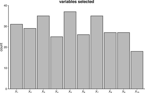
As mentioned earlier, a uniform distribution is typically employed as the prior for selecting splitting variables, resulting in an equal probability for each variable to be chosen. Through logical inference or background analysis, we may identify certain variables as more important than others in specific models. In such cases, it is necessary to assign higher probabilities to these variables, such as the time variable in a time-related model or location variables in a spatial-related model. In these situations, simply applying the BART model fails to fully utilize this prior knowledge. We applied the BART model to the data generated from scenario $F_1(x)$ in Section 4.1 in which we can find that $x_1$ is related to each part of the function, so it is a natural idea to force $x_1$ to be in every regression tree. Figure 1 illustrates the frequency of each variable in the model during the final iteration. It reveals that the important variable $x_1$ is not the most frequently selected; on the contrary, certain irrelevant variables like $x_7$ exhibit higher frequencies than $x_1$.

Figure 1. The frequency of each variable used in the BART model. $X_1$ is an important variable. $X_6,\dots ,X_{10}$ are irrelevant variables.

When we possess such prior knowledge, we can anchor these variables at the topmost levels of the trees. Note that in the case of ordinal splitting variables, samples with $x\le c$ (where c represents the cut point for the splitting variable) are directed to the left child node, while samples with x>c are assigned to the right child node. When there is a need to fix multiple layers of variables, it is common to assign the same splitting variable to the left and right child nodes, thus establishing variable fixing across layers. For instance, if we identify two variables as crucial in the model, we can fix these two variables at the topmost two levels of the trees, effectively preventing other variables from appearing at these levels.

The four moves for generating a new tree structure are modified.

1. Grow: If a node in the fixed layers needs to be grown, only the assigned important variables are allowed to be chosen as splitting variables.

2. Prune: No changes are made unless a logical hyperparameter is in effect. Detailed information will be provided later.

3. Swap: The tree structure will not be changed if swapping two nodes violates the rule.

4. Change: If a node in the fixed layer needs to be changed, the variable to be split is confined to the fixed variable scope.

The details of PFBART can be referred to in Algorithm 1.

Three logical hyperparameters are introduced in PFBART to enhance control over the fixing activity.

The first logical hyperparameter, $\mathtt{\text{Prune}}$, controls the prune process. If Prune is False and the node to be pruned is in the fixed layers, the prune process will not alter the tree structure.

When dealing with multiple important variables, fixing each layer with each variable may be too demanding. If Swap is True, these variables can appear at any fixed layer. Otherwise, the variables to be fixed must follow a specific order. Specifically, the first important variable can only be selected in the first layer of the trees, and so on.

Given the BART model's restriction on tree depth, fixing multiple variables at the tree's upper levels may hinder the inclusion of other variables in lower level. Therefore, we introduce a logical parameter called ChangePrior. When ChangePrior is False, we maintain the splitting probability unchanged. If ChangePrior is True, nodes in the fixed layers adopt the same splitting probability as the root node of the trees. Nodes outside the fixed layers undergo a probability adjustment to $\alpha (1+d-h{)}^{-\beta }$, where h denotes the height of the fixed layers.

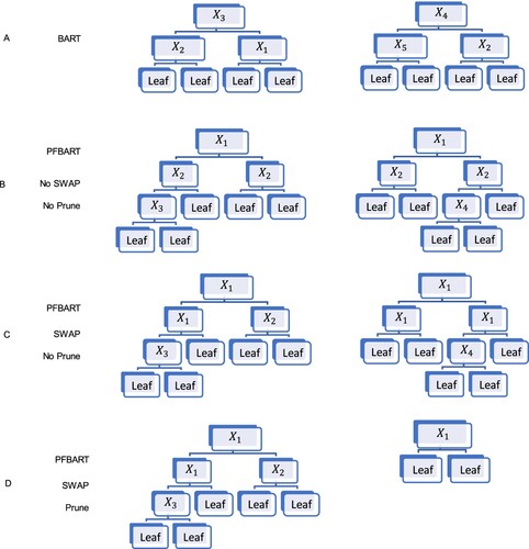
A toy example is used to demonstrate PFBART and the effect of the logical hyper parameter. We used data generated from scenario $F_1(x)$. We take two trees from the two hundred trees as a brief example. If we use BART model to fit the data, $X_1$ may not be in every regression tree which we can see from the second tree of part A of Figure 2. $X_1$ and $X_2$ are two variables we fix in PFBART($X_2$ is fixed just to demonstrate the effect of hyper parameter). In part B of Figure 2, we set Swap as false, which means the order is fixed. In our example we fix $X_1$ at the first layer and $X_2$ at the second layer of the regression tree. In part C, Swap is true, so the variable in the first two layers must be $X_1$ or $X_2$ and they don't have to be in special order. By setting Prune to true in part D, the second tree exhibits a single-layer tree structure. In contrast, in parts B and C, the tree structure always consists of more than one layer.

Figure 2. Toy example for PFBART.

4. Illustrations

4.1. Simulation experiment

Initially, we illustrate the advantages of PFBART over BART in various scenarios. The data is generated based on function $F_1(X)=10\sin (\pi X_1{X}_2)+5X_1^2(X_3-0.5)+10X_1^3{X}_3{X}_4+5X_1^4{X}_5.$To make comparation, considering another two scenarios which data is generated from functions $F_2(X)=10\sin (\pi X_1{X}_2)+5X_2^2(X_3-0.5)+10X_1^3{X}_3{X}_4+5X_1^4{X}_5$and $F_3(X)=10\sin (\pi X_6{X}_2)+5X_6^2(X_3-0.5)+10X_6^3{X}_3{X}_4+5X_6^4{X}_5.$In scenario $F_1(x)$, $X_1$ is associated with every part of the function, indicating its crucial role. In scenario $F_2(x)$, the second part is unrelated to $X_1$, enabling us to evaluate PFBART's performance when the fixed variable is less significant. In scenario $F_3(x)$, $X_1$ is an irrelevant variable in the model. To demonstrate that PFBART's effectiveness is independent of the variable selection process, we run the model exclusively with $X_1,\dots ,X_5$ using data from $F_1(x)$. This scenario is labelled as $F_4(x)$.

We generate 100 datasets for each function, with a sample size of 4000 in each dataset. Each dataset comprises 10 variables, $X_1,\dots ,X_{10}$, randomly sampled from a uniform distribution $U(0,1)$. The datasets are split equally into training and testing subsets. In both BART and PFBART, the initial 500 unstable iterations are excluded, and the following 1000 iterations are considered as the model result. The remaining parameters utilize the default settings.

Each function was employed to predict the corresponding test set based on its respective training set. The predictions were evaluated using the root mean squared error (RMSE), $\mathrm{RMSE}=\sqrt{\frac{1}{2000}\sum _{i=1}^{2000}{(\hat{f}\left(x_i\right)-f\left(x_i\right))}^2}.$In this experiment, two competitors of eXtreme Gradient Boosting (XGB) and random forests (RF) with the default settings are introduced. We can see that BART outperforms XGB and RF in the four scenarios which means the two competitors can not recognize this special structure, so we mainly focus on the comparison of BART and PFBART in this section.

Table 1 lists the four combinations of logical hyper parameter with which we conduct PFBART. Figure 3 shows the boxplots of the 100 RMSE values for each scenario.

Figure 3. Boxplots of the RMSE values for each method across the 100 data sets.

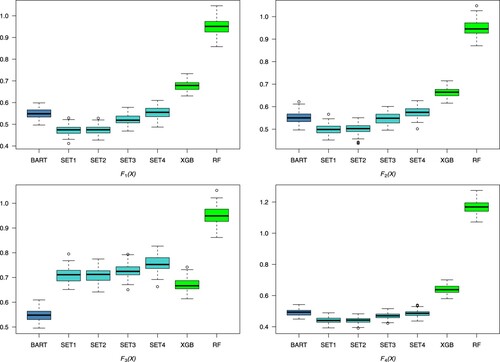
Table 1. Settings for hyperparameter.

	ChangePrior	Prune
SET1	False	True
SET2	False	False
SET3	True	True
SET4	True	False

Some finding can be derived from Figure 3.

1. The performance of different logical parameters follows a specific order in the four scenarios: SET1 ≈ SET2 > SET3 > SET4. Setting the logical parameter ChangePrior to True is a trade-off for easier growth of deeper trees at the cost of overfitting. When there is only one layer to fix, changing the splitting priority is unnecessary and leads to overfitting. When ChangePrior is True, setting the logical parameter Prune to False increases the probability of overfitting. However, when the splitting priority remains unchanged, allowing or disallowing pruning in the fixed layer has little effect on the model. There is almost no difference between SET1 and SET2. Therefore, the following discussion primarily focuses on comparing PFBART SET1 and BART.

2. In scenario $F_1(X)$, PFBART reduces the median RMSE by approximately $15\mathrm{\%}$ compared to BART. This indicates that if we possess right prior information that the fixed variable is related to every part of the model, PFBART can archive more accurate estimations.

3. In scenario $F_2(X)$, where a portion of the model is unrelated to the assigned fixed variable $X_1$, PFBART reduces the median RMSE by approximately $9\mathrm{\%}$. This suggests that PFBART can perform effectively in a wider range of scenarios as long as the fixed variable is correlated with large part of the model.

4. In scenario $F_3(X)$, where the fixed variable $X_1$ is irrelevant to the model, PFBART performs poorly due to fixing an irrelevant variable, which introduces additional error to the model.

5. In scenario $F_4(X)$, where only $X_1,\dots ,X_5$ are used in the model, PFBART still outperforms BART by approximately $10\mathrm{\%}$. This indicates that the effectiveness of PFBART is not solely attributed to the variable selection process.

4.2. UCI data sets

In the previous simulation, we demonstrated how prior knowledge can be utilized to achieve better estimations. In this section, we illustrate the use of PFBART on data without prior knowledge.

From the UCI dataset (Dua & Graff, 2017), we selected 14 datasets based on the following criteria. (1) Sample size ranging from 240 to 5500. (2) Attributes ranging from 5 to 13. (3) Regression datasets, excluding time series datasets. The details of the datasets can be referred to in Table 2.

Table 2. UCI data sets information.

Data set name	Size	Covariate
Abalone	4170	8
Airfoil Self Noise	1500	5
Auto MPG	390	8
Bike Rental	730	10
Concrete Compressive Strength	1030	8
Energy Efficiency	760	8
Forest Fire	510	12
QSAR Aquatic Toxicity	540	8
QSAR Fish Toxicity	900	6
Real Estate Valuation	410	7
Strike	620	6
Tecator	240	13
Wine Quality	4890	11
Yacht Hydrodynamics	300	6

For simplification purposes, we randomly removed samples from the dataset to ensure that the total sample size is divisible by 10. Each dataset was evaluated using 10-fold cross-validation. We performed 10 randomizations for each dataset. Each variable is fixed at the top of the trees. We used the relative RMSE, defined as the ratio of PFBART RMSE to BART RMSE for the same dataset, as a measure of variable importance. Thus we obtained 10 such statistics for each covariate, presented in Figure 4.

Figure 4. Relative RMSE for every covariate in UCI data sets.

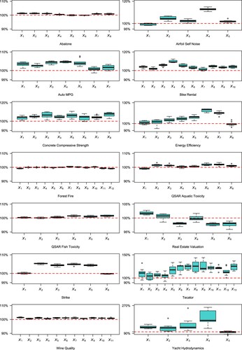
For the datasets Abalone, Forest Fire, Wine Quality, QSAR Aquatic Toxicity, and QSAR Fish Toxicity, fixing every variable had a similar effect on the BART model. This suggests that these variables all contribute to the model, and no single variable plays a dominant role.

For the Airfoil Self Noise dataset, the variable $X_1$, frequency, is highly correlated with the dependent variable sound pressure level, as observed in Brooks et al. (1989).

In the Auto MPG dataset, the variable $X_6$ (model year) is an important variable in the model, as it reflects changes in the MPG model due to scientific and technological advancements over different model years.

In the Bike Rental dataset, two variables, $X_2$ (month) and $X_7$ (feeling temperature), interact with other independent variables to influence bike rental behaviour.

For the Concrete Compressive Strength dataset, fixing each variable results in slightly worse estimation. However, these variables are not irrelevant variables, so we can incorporate this information along with background knowledge for future use.

In the Energy Efficiency dataset, $X_8$ (Glazing Area Distribution) is an important variable as different types of area distributions lead to different energy efficiency models.

In the Real Estate Valuation dataset, fixing $X_5$ (latitude) and $X_6$ (longitude) improves estimation accuracy. Considering the common knowledge that these variables interact with other variables such as $X_1$ (transaction date) and $X_2$ (house age) to predict house prices, the results seem reasonable. In the next section, we will examine the performance of PFBART on a larger real estate dataset.

In the Strike dataset, the two important variables, $X_1$ (country) and $X_6$ (union centralization), interact with other independent variables to influence the strike volume.

The Tecator dataset is used to predict the fat content of a meat sample based on its near-infrared absorbance spectrum. The dependent variables are principal components derived from the spectrum. No dominant variable can be identified among the principal components, although the first four components appear to be more important than others.

In the Yacht Hydrodynamics dataset, fixing $X_5$ (Froude number) improves the estimation. Based on background information in hydrodynamics, $X_5$ plays a significant role in predicting residuary resistance. Fixing other covariates except $X_5$ leads to worse estimation, especially for $X_4$. However, removing $X_4$ from the model also results in worse estimation, suggesting that $X_4$ should be included in the model. It is not a variable with global influence, similar to $X_4$ in the Airfoil Self Noise and Bike Rental datasets. This indicates that variables with high relative RMSE are not necessarily useless in the model.

4.3. Beijing housing price

The Beijing house price data (Lin et al., 2023) is used to demonstrate the process of fixing multiple variables in a spatial-temporal model. The response variable is the unit house price, and the covariates include location, floor, number of living rooms and bathrooms, presence of an elevator, and other variables. Based on prior knowledge, we assume that location and year of trading have a significant influence on the model. In this study, the longitude, latitude, and year of trading are fixed at the top three layers of the regression trees.

After preprocessing, the dataset consists of 296255 valid samples. Due to the large sample size and the time-consuming nature of MCMC iterations, a random selection of $30\mathrm{\%}$ of the total samples is used for training, while the remaining $70\mathrm{\%}$ is used for testing. This process generates 10 datasets, and for each dataset, PFBART is run with eight combinations of logical hyperparameters, as listed in Table 3. The relative RMSE is used as the evaluation metric.

Table 3. Hyper parameter combinations.

	ChangePrior	Prune	Swap
SET1	True	True	False
SET2	True	True	True
SET3	False	False	False
SET4	False	False	True
SET5	True	False	False
SET6	True	False	True
SET7	False	True	False
SET8	False	True	True

Figure 5 presents the results of eight different PFBART models with varying hyperparameter settings. All eight models outperform BART, with SET6 yielding the best performance.

Figure 5. Relative RMSE for PFBART with Beijing house price data.

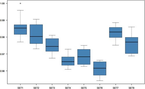
The results confirm our hypothesis that spatial-temporal variables play a crucial role in the model. In other words, a significant portion of the variance in house prices is related to these three variables.

The good performance of SET6 can be explained as follows.

1. Fixing multiple layers in the tree has the side effect of making it difficult for other covariates to be included in the model. To address this, we can adjust the splitting probability in a way that allows non-fixed layers to grow as if without the fixed layers, thus facilitating deeper growth.

2. Preventing nodes from being pruned results in regression trees with more than two layers. Conversely, including pruning may lead to unexpected shallow trees that do not align with our expectations.

3. When fixing more than one layer, should the order of fixing be considered? By setting Swap to True, we can relax this restriction and make the model more flexible to approximate the true model effectively. This change allows the three variables (longitude, latitude, and year of trading) to grow at the fixed layers without considering their order.

5. Conclusion and looking forward

When constructing statistical models, particularly those related to spatial-temporal analysis, it is known that certain variables have a strong correlation with the majority of the model either through logical deduction or background knowledge. This paper presents a method, referred to as Partially Fixed BART, that leverages this prior knowledge by fixing these important variables at the top of the regression trees. Through data experiments and real-world examples, it is demonstrated that this approach leads to improved performance compared to the original BART model. Additionally, even in the absence of prior information, the proposed model can still be employed to achieve more accurate estimations or serve as a measure of variable importance.

The primary contribution of this paper is the development of PFBART, an extension of the BART model. In a previous work by Linero and Yang (2018), a soft BART model was introduced, which is better suited for approximating continuous or differentiable functions. Building upon this, we plan to incorporate the fixing of important variables based on the soft BART model and investigate whether this modification yields further improvement.

PFBART demonstrates superior performance in datasets where certain dominant variables exert significant influence. However, in most scenarios, each variable is only correlated with a portion of the overall variation, and there is no dominant variable. Currently, we are focussed on analysing the model structure and leveraging this information to enhance its performance.

Acknowledgements

The authors are grateful to the Editor, an Associate Editor and two anonymous referee for their insightful comments and suggestions on this article, which have led to significant improvements.

Disclosure statement

No potential conflict of interest was reported by the author(s).

References

- Breiman, L. (2001). Random forests. Machine Learning, 45(1), 5–32. https://doi.org/10.1023/A:1010933404324
- Brooks, T. F., Pope, D. S., & Marcolini, M. A. (1989). Airfoil self-noise and prediction [Tech. Rep]. NASA.
- Chen, T., & Guestrin, C. (2016). Xgboost: A scalable tree boosting system. In Proceedings of the 22nd ACM SIGKDD International Conference on Knowledge Discovery and Data Mining (pp. 785–794). Association for Computing Machinery.
- Chipman, H. A., George, E. I., & McCulloch, R. E. (2010). BART: Bayesian additive regression trees. The Annals of Applied Statistics, 4(1), 266–298. https://doi.org/10.1214/09-AOAS285
- Dua, D., & Graff, C. (2017). UCI machine learning repository. https://archive.ics.uci.edu/ml
- Lin, W., Shi, Z., Wang, Y., & Yan, T. H. (2023). Unfolding Beijing in a hedonic way. Computational Economics, 61(1), 1–24. https://doi.org/10.1007/s10614-021-10209-3
- Linero, A. R. (2018). Bayesian regression trees for high-dimensional prediction and variable selection. Journal of the American Statistical Association, 113(522), 626–636. https://doi.org/10.1080/01621459.2016.1264957
- Linero, A. R., & Yang, Y. (2018). Bayesian regression tree ensembles that adapt to smoothness and sparsity. Journal of the Royal Statistical Society Series B: Statistical Methodology, 80(5), 1087–1110. https://doi.org/10.1111/rssb.12293
- Tan, Y. V., & Roy, J. (2019). Bayesian additive regression trees and the general BART model. Statistics in Medicine, 38(25), 5048–5069. https://doi.org/10.1002/sim.v38.25