Statistical inference of reliability for a K-out-of-N: G system with switching failure under Poisson shocks

Abstract

Based on the stochastic uncertainty of the system's operating environment, this research presents statistical inferences on the mean time to failure (MTTF) of a K-out-of-N: G non-repairable system model with switching failure under Poisson shocks. The standby component is switched to the operating component when an operating component fails, with a switching failure probability of p. The MTTF of the system is derived by using the Markov process theory and the Laplace transform for two cases where the shock threshold is a constant value or a random variable. The maximum likelihood estimator (MLE) of the MTTF is obtained, and based on this estimator, asymptotic confidence interval estimation and hypothesis testing are performed. Based on the setting of the basic parameter values, the MTTF under two different cases of the shock threshold is compared. The effect of each parameter on the MTTF is analyzed in numerical simulation. The effectiveness of the above statistical inference methods is also verified by numerical simulation.

Keywords:

• Poisson shock
• switching failure
• mean time to failure
• hypothesis testing
• asymptotic confidence interval

1. Introduction

The redundancy technology of standby components can improve system reliability. In reliability research and engineering, the k-out-of-n: G system with standby components is a general redundant system, where n denotes the number of components in the system, and the system can operate normally when the number of operating components in the system is not less than k. Generally speaking, the kinds of standby can be divided into cold standby, warm standby and hot standby. The k-out-of-n: G system with mixed cold and warm standby components is considered in this paper. Based on the different standby types of standby components, some scholars have used diverse methods to model and analyze the reliability of k-out-of-n: G non-repairable systems. By using the Markov model, Pham and Pham (1991) deduced a closed-form solution of the instantaneous probability for a k-out-of-n: G non-repairable system with two failure modes. For a k-out-of-n: G non-repairable warm standby system with completely reliable switching, She and Pecht (1992) developed a general closed-form equation of the system reliability. Amari and Dill (2009) proposed an approach of k logical locations, which can effectively analyze the reliability of non-repairable systems with cold or warm standby and general failure time distributions. Boddu and Xing (2012) proposed a system model composed of s-independent k-out-of-n: G mixed standby subsystems connected in series. Baek and Jeon (2013) considered the optimization problem for a k-out-of-n: G system with mixed redundancy.

For redundant standby systems, the standby component may fail during the switchover process. For example, a standby generator in a plant power supply system may fail during switching from the standby to the operating one due to some complex physical reasons. Lewis (1996) introduced standby switching failure into the study of system reliability for the first time. Ke et al. (2008) focused on reliability and sensitivity for a repairable system with switching failure. Wang and Chen (2009) studied a repairable system with general repair time, reboot delay and switching failure. Hsu et al. (2014) investigated the maintenance of a warm standby machine and considered the switching failure of standby components and maintenance stress coefficient. Ke et al. (2016) analyzed the performance metrics and optimization of a machine maintenance system with standby switching failure. Shekhar et al. (2020) performed the reliability analysis for warm standby nodes provisioning computing network system with switching failure, vacation interruption and common cause failure. Yang and Wu (2021) performed some reliability research for a standby repairable system with working breakdown and switching failure. In Liu et al. (2022), a cost-benefit analysis of standby retrial systems with unreliable servers and switching failure was carried out. Given that the study for k-out-of-n: G non-repairable systems with mixed standby components rarely involves standby switching failure, and this failure situation does exist in engineering, the possibility of switching failure is considered in this paper.

In practical engineering, system components fail not only due to their lifetime, but also due to the impact of external random environment which is usually regarded as a shock. With the increasing requirements for evaluating the operation of system equipment in a stochastic environment, shock models are becoming more widely studied in the field of reliability. Barlow and Proschan (1975) elaborated on the problem of the lifetime distribution of single-component systems under Poisson shocks. Shanthikumar and Sumita (1983, 1984) proposed a class of shock model which is usually used to study seismic and inventory problems, and considered two cases where the system fails when the cumulative shock magnitude or a single shock magnitude exceeds the threshold, respectively. Wu and Wu (2011) studied a two-unit cold standby repairable system under Poisson shocks. The external shocks only affect the operating unit and the failure of the unit is only caused by external shocks. In addition to the failure of the unit caused by external shocks, Wu (2012) also considered the failure of the unit caused by the unit's lifetime, and then obtained optimal replacement strategies for a two-unit cold standby system. Wu et al. (2015) conducted the reliability analysis of a multi-unit cold standby system in which both the operating unit and the transfer switch are affected by external shocks. El-Sherbeny and Elshoubary (2020) investigated the reliability of a parallel system which consists of two different components and a repairer, in which the failure of the system is caused by external shocks. Ge et al. (2021) considered a cold standby repairable system model under a stepped Poisson shock whose strength varies with the number of failures of operating components. El-Sherbeny and Hussien (2022) studied the reliability of a parallel system under Poisson shocks where the repairer has an optional vacation. Based on the failure mechanism of components in a stochastic environment, in this paper, the failure of the operating component is caused by its lifetime or Poisson shocks.

In the evaluation of system reliability, the parameters in some distribution functions involved and various system reliability indices are generally not directly available. Therefore, many scholars have used statistical methods to infer the system reliability such as Kızılaslan (2018), Wang et al. (2020) and Rasekhi et al. (2020). Statistical inference is always used to estimate the parameters/characteristics of a system by using experimental data or simulated data. Patawa et al. (2022) analyzed the reliability of cold standby systems whose repair time follows the Lindley distribution, and estimated unknown parameters by using two methods of maximum likelihood and Bayesian. Kang et al. (2023) studied the availability of a repairable retrial system with warm standby and priority, and estimated the system parameters using the Bayesian method. In previous studies on the statistical inference of the reliability of standby systems, most scholars considered the standby systems whose switching is completely reliable. For the statistical inference for the system availability/reliability with switching failure mechanism, Hsu et al. (2011) derived the expression for the steady-state availability of three-component systems with unreliable repairer and switching failure, and carried out maximum likelihood estimation and hypothesis testing. However, Hsu et al. (2011) did not consider using the Bayesian method to infer the reliability of this system. After that, Ke et al. (2018) carried out Bayesian inference on the system model studied in the literature (Hsu et al., 2011) based on two different types of repair time distributions respectively. For the problem of statistical inference for k-out-of-n systems, based on Weibull and Burr-III distributions, Ali et al. (2018) performed reliability inference for a s-out-of-k: G system stress-strength model using two methods, namely, maximum likelihood and Bayesian. Jana and Bera (2022) carried out a study for constructing various estimation intervals of the stress-strength reliability of k-out-of-n: G systems. Chien et al. (2006) estimated the asymptotic confidence interval of the steady-state availability and the MTTF of a k-out-of-m + s: G repairable system with an imperfectly reliable server. However, no literature has investigated the problem of statistical inference on the reliability of k-out-of-n systems with switching failure and mixed standby components.

The influence of the external environment on the operating components and the switching failure of standby components in actual engineering are considered in this paper. Hence, Poisson shock and switching failure are introduced into k-out-of-n: G non-repairable systems, and then a new reliability model of the k-out-of-n: G system with mixed standby components is constructed. In practical engineering, system reliability index is always a function containing component parameters. The analysis of system reliability is essentially an inference of the system reliability index by using statistical methods. No statistical inference has been made about the reliability characteristics of k-out-of-n: G systems with switching failure, which motivates us to explore the problem of statistical inference for the reliability of k-out-of-n: G systems with switching failure. Therefore, this work intends to investigate the statistical inference of the reliability of a k-out-of-n: G system with switching failure under Poisson shocks. The used methods are classical statistics and Monte Carlo simulation. This work can provide a scientific theory and a method for reliability assessment and quality management of k-out-of-n: G systems.

The rest of this paper is structured as follows. The considered system model is described in detail and some assumptions are given in Section 2. Furthermore, the model is analyzed and the recursive expression of the MTTF is obtained. Section 3 is devoted to the statistical inference of the MTTF. Numerical simulation studies are presented to verify the performance of the statistical inference method in Section 4. In addition, the influence of system parameters on the MTTF is analyzed, and the MTTF under two different threshold conditions is compared. The conclusions and some suggestions for future research are given in Section 5.

2. System modeling and analysis

2.1. Model description

The considered system operates in an environment with Poisson shocks. The system is composed of N components, including M identical operating components, W identical warm standby components, and C identical cold standby components. The failed components cannot be repaired. Once the number of operating components in the system is less than K, the system fails. The system is noted as a K-out-of-N: G non-repairable system. After the system fails, the components in the system will not continue to fail. The specific assumptions of this system model are given as follows.

1. All components fail independently.

2. At time t = 0, M components are operating and all components are new.

3. The operating component in the system is affected by the lifetime of the component itself or external shocks. The lifetime X of each operating component and the standby lifetime Y of each warm standby component are assumed to be exponentially distributed with parameters ${\lambda }_a$ and $\beta (0<\beta <{\lambda }_a)$, respectively. The system is subjected to the shock from a homogeneous Poisson flow with the shock intensity of ${\lambda }_b$. In other words, the arrival interval U of the shocks follows the exponential distribution with parameter ${\lambda }_b$.

4. Each shock affects the components independently of each other, only the operating components are affected by the shock, and the shock does not affect the standby components. The magnitude $\hat{Z}$ of each shock follows a distribution with the cumulative distribution function F. The threshold is the same for each operating component. If the magnitude $\hat{Z}$ of each shock exceeds the threshold, the component will fail.

5. If an operating component fails, a standby component is switched to an operating component instantly, and the warm standby component is switched preferentially. The switching time is negligible.

6. In the process of component switching, the standby components may fail with a failure probability of $p(0\le p\le 1)$. As long as there are standby components when the switching fails, the switching will continue until it is successful.

7. All the random variables in this model are independent of each other.

For different working environments of the system, the following two cases are considered, where the threshold is a constant value or a random variable.

Case 1: The threshold is a constant value υ.

From assumptions (3) and (4), the failure probability of a single component due to a shock is (1) $P_{\hat{Z}}=\mathrm{P}(\hat{Z}>\upsilon )=1-\mathrm{P}(\hat{Z}\le \upsilon )=1-F(\upsilon )=\overline{F}(\upsilon ).$(1) The event $A_{\mathrm{rs}}$ represents that a shock causes the specified s−r components among the M−r operating components in the system to fail, and the remaining M−s operating components are normal. We note that r and s ($s\ge r$) represent the numbers of failed operating components before and after shock, respectively. The $a_{\mathrm{rs}}$ represents the probability of occurrence of $A_{\mathrm{rs}}$, and then (2) $a_{\mathrm{rs}}=\mathrm{P}(A_{\mathrm{rs}})=F(\upsilon {)}^{M-s}\overline{F}(\upsilon {)}^{s-r}.$(2) Assuming that the distribution of the shock magnitude $\hat{Z}$ is an exponential one with the parameter u, then Equation (2(2) $a_{\mathrm{rs}}=\mathrm{P}(A_{\mathrm{rs}})=F(\upsilon {)}^{M-s}\overline{F}(\upsilon {)}^{s-r}.$(2) ) can be expressed as (3) $a_{\mathrm{rs}}=(1-{\mathrm{e}}^{-\mathrm{u\upsilon }}{)}^{M-s}({\mathrm{e}}^{-\mathrm{u\upsilon }}{)}^{s-r}.$(3)

Case 2: The threshold is a random variable V, which follows a distribution with the cumulative distribution function φ.

From assumptions (3) and (4), the failure probability of a single component is $P_{\hat{z}}=\mathrm{P}(V\le \hat{z})=\phi (\hat{z})$ when the value of the shock magnitude is $\hat{z}$. Let $H=\phi (\hat{Z})$, and then (4) $\mathrm{P}(H\le h)=\mathrm{P}(\phi (\hat{Z})\le h)=\mathrm{P}(\hat{Z}\le {\phi }^{-1}(h))=F({\phi }^{-1}(h))=F{\phi }^{-1}(h).$(4) Let $D(h)=F{\phi }^{-1}(h)$ be the distribution function of H, and then we have (5) $a_{\mathrm{rs}}={\int }_0^1\mathrm{P}(A_{\mathrm{rs}}|H=h)\mathrm{d}D(h)={\int }_0^1(1-h{)}^{M-s}{h}^{s-r}\mathrm{d}D(h).$(5) Assuming that the distribution function F is the same as the distribution function φ, then the distribution of H is a uniform distribution on the interval (0, 1). Then, Equation (5(5) $a_{\mathrm{rs}}={\int }_0^1\mathrm{P}(A_{\mathrm{rs}}|H=h)\mathrm{d}D(h)={\int }_0^1(1-h{)}^{M-s}{h}^{s-r}\mathrm{d}D(h).$(5) ) can be expressed as (6) $a_{\mathrm{rs}}={\int }_0^1(1-h{)}^{M-s}{h}^{s-r}\mathrm{d}h=\mathrm{Beta}(M-s+1,s-r+1).$(6)

2.2. System state analysis

At time t, let $N(t)=i(i=0,1,\dots ,N)$ represent the number of failed components in the system. According to the model description, the state of the system at time t is denoted by $\{N(t),t\ge 0\}$, which constitutes a continuous-time homogeneous Markov process with the state space $\mathrm{\Omega }=T\cup \mathit{\Psi }$, where $T=\{0,1,\dots ,N-K\}$ and $\mathit{\Psi }=\{N-K+1,N-K+2,\dots ,N\}$ are the set of working states and the set of failure states, respectively.

The state probability of the system at time t is defined as follows. $P_i(t)=\mathrm{P}\{N(t)=i\},i=0,1,\dots ,N.$Therefore, the vector of the state probability of the system is $\mathit{P}(t)=(P_0(t),P_1(t),\dots ,P_N(t)).$Let ${\lambda }_{i,j}$, ${\varphi }_{i,j}$, ${\theta }_{i,j}$, ${\delta }_{i,j}$ and ${\gamma }_{i,j}$ represent the transition rates of the number of failed components in the system from i to j under different conditions, respectively. The transition rates between the states of the system are given as follows.

1. When the number of failed components in the system is i, one component fails due to shock or its lifetime. Then the transition rate is given by ${\lambda }_{i,i+1}=\{\begin{array}{ll}M{\lambda }_a(1-p)+(W-i)\beta +M{a}_{01}{\lambda }_b(1-p),& 0\le i\le W-1,\\ M{\lambda }_a(1-p)+M{a}_{01}{\lambda }_b(1-p),& W\le i\le W+C-1,\\ (N-i){\lambda }_a+(N-i)a_{i-(W+C),i-(W+C)+1}{\lambda }_b,& W+C\le i\le N-K,\\ 0,& \mathrm{otherwise}.\end{array}$

2. When the number of failed components in the system is i and there are standby components, that is $0\le i\le W+C-1$, multiple components fail due to shock and switching failure. Then the transition rate is given as follows.

   • When $2+i\le j\le W+C$, ${\varphi }_{i,j}=\{\begin{array}{ll}{\displaystyle M{\lambda }_a{p}^{j-i-1}(1-p)+\sum _{d=1}^{j-i}(\genfrac{}{}{0ex}{}{M}{d})a_{0d}{\lambda }_b{p}^{j-i-d}(1-p{)}^d,}& j-i\le M,\\ {\displaystyle M{\lambda }_a{p}^{j-i-1}(1-p)+\sum _{d=1}^M(\genfrac{}{}{0ex}{}{M}{d})a_{0d}{\lambda }_b{p}^{j-i-d}(1-p{)}^d,}& j-i>M.\end{array}$

   • When j = W + C + 1, ${\theta }_{i,j}=\{\begin{array}{ll}{\displaystyle M{\lambda }_a{p}^{j-i-1}+\sum _{d=1}^{j-i}(\genfrac{}{}{0ex}{}{M}{d})a_{0d}{\lambda }_b{p}^{j-i-d}(1-p{)}^{d-1},}& j-i\le M,\\ {\displaystyle M{\lambda }_a{p}^{j-i-1}+\sum _{d=1}^M(\genfrac{}{}{0ex}{}{M}{d})a_{0d}{\lambda }_b{p}^{j-i-d}(1-p{)}^{d-1},}& j-i>M.\end{array}$

   • When $W+C+1<j\le N$, ${\delta }_{i,j}=\{\begin{array}{ll}{\displaystyle \sum _{d=j-(W+C)}^{j-i}(\genfrac{}{}{0ex}{}{M}{d})a_{0d}{\lambda }_b{p}^{j-i-d}(1-p{)}^{W+C-j+d},}& j-i\le M,\\ {\displaystyle \sum _{d=j-(W+C)}^M(\genfrac{}{}{0ex}{}{M}{d})a_{0d}{\lambda }_b{p}^{j-i-d}(1-p{)}^{W+C-j+d},}& j-i>M.\end{array}$

3. When the number of failed components in the system is i and there are no standby components, that is $W+C\le i\le N-K$, multiple components fail due to shock. Then the transition rate is given by ${\gamma }_{i,j}=(\genfrac{}{}{0ex}{}{N-i}{j-i})a_{i-(W+C),j-(W+C)}{\lambda }_b,2+i\le j\le N.$

2.3. State transition rate matrix of the system

The state transition rate matrix $\mathit{Q}$ of the system can be divided into block matrices according to the existence situation of standby components, the situation of standby switching, and the system working state, so $\mathit{Q}$ is represented as follows: $\mathit{Q}=\left(\begin{array}{cccc}{\mathit{Q}}_{11}& {\mathit{Q}}_{12}& {\mathit{Q}}_{13}& {\mathit{Q}}_{14}\\ {\mathit{Q}}_{21}& {\mathit{Q}}_{22}& {\mathit{Q}}_{23}& {\mathit{Q}}_{24}\\ {\mathit{Q}}_{31}& {\mathit{Q}}_{32}& {\mathit{Q}}_{33}& {\mathit{Q}}_{34}\\ {\mathit{Q}}_{41}& {\mathit{Q}}_{42}& {\mathit{Q}}_{43}& {\mathit{Q}}_{44}\end{array}\right),$where $\mathit{Q}$ is a square matrix of order N + 1.

The subblocks in the matrix $\mathit{Q}$ are as follows: $\begin{array}{rl}{\mathit{Q}}_{11}& ={\left(\begin{array}{ccccccc}{\lambda }_{0,0}& {\lambda }_{0,1}& {\varphi }_{0,2}& {\varphi }_{0,3}& \cdots & {\varphi }_{0,W+C-1}& {\varphi }_{0,W+C}\\ 0& {\lambda }_{1,1}& {\lambda }_{1,2}& {\varphi }_{1,3}& \cdots & {\varphi }_{1,W+C-1}& {\varphi }_{1,W+C}\\ 0& 0& {\lambda }_{2,2}& {\lambda }_{2,3}& \cdots & {\varphi }_{2,W+C-1}& {\varphi }_{2,W+C}\\ 0& 0& 0& {\lambda }_{3,3}& \cdots & {\varphi }_{3,W+C-1}& {\varphi }_{3,W+C}\\ ⋮& ⋮& ⋮& ⋮& \ddots & ⋮& ⋮\\ 0& 0& 0& 0& \cdots & {\lambda }_{W+C-1,W+C-1}& {\lambda }_{W+C-1,W+C}\\ 0& 0& 0& 0& \cdots & 0& {\lambda }_{W+C,W+C}\end{array}\right)}_{(W+C+1)\times (W+C+1)},\\ {\mathit{Q}}_{12}& ={\left(\begin{array}{c}{\theta }_{0,W+C+1},\dots ,{\theta }_{W+C-1,W+C+1},{\lambda }_{W+C,W+C+1}\end{array}\right)}_{(W+C+1)\times 1}^{\mathrm{\top }},\\ {\mathit{Q}}_{13}& ={\left(\begin{array}{cccc}{\delta }_{0,W+C+2}& {\delta }_{0,W+C+3}& \cdots & {\delta }_{0,N-K}\\ {\delta }_{1,W+C+2}& {\delta }_{1,W+C+3}& \cdots & {\delta }_{1,N-K}\\ ⋮& ⋮& \ddots & ⋮\\ {\delta }_{W+C-1,W+C+2}& {\delta }_{W+C-1,W+C+3}& \cdots & {\delta }_{W+C-1,N-K}\\ {\gamma }_{W+C,W+C+2}& {\gamma }_{W+C,W+C+3}& \cdots & {\gamma }_{W+C,N-K}\end{array}\right)}_{(W+C+1)\times (M-K-1)},\\ {\mathit{Q}}_{14}& ={\left(\begin{array}{cccc}{\delta }_{0,N-K+1}& {\delta }_{0,N-K+2}& \cdots & {\delta }_{0,N}\\ {\delta }_{1,N-K+1}& {\delta }_{1,N-K+2}& \cdots & {\delta }_{1,N}\\ ⋮& ⋮& \ddots & ⋮\\ {\delta }_{W+C-1,N-K+1}& {\delta }_{W+C-1,N-K+2}& \cdots & {\delta }_{W+C-1,N}\\ {\gamma }_{W+C,N-K+1}& {\gamma }_{W+C,N-K+2}& \cdots & {\gamma }_{W+C,N}\end{array}\right)}_{(W+C+1)\times K},\\ {\mathit{Q}}_{21}& ={\mathbf{0}}_{1\times (W+C+1)},{\mathit{Q}}_{22}=\left(\begin{array}{c}{\lambda }_{W+C+1,W+C+1}\end{array}\right),\\ {\mathit{Q}}_{23}& ={\left(\begin{array}{c}{\lambda }_{W+C+1,W+C+2},{\gamma }_{W+C+1,W+C+3},\dots ,{\gamma }_{W+C+1,N-K}\end{array}\right)}_{1\times (M-K-1)},\\ {\mathit{Q}}_{24}& ={\left(\begin{array}{c}{\gamma }_{W+C+1,N-K+1},{\gamma }_{W+C+1,N-K+2},\dots ,{\gamma }_{W+C+1,N}\end{array}\right)}_{1\times K},\\ {\mathit{Q}}_{31}& ={\mathbf{0}}_{(M-K-1)\times (W+C+1)},{\mathit{Q}}_{32}={\mathbf{0}}_{(M-K-1)\times 1},\\ {\mathit{Q}}_{33}& ={\left(\begin{array}{cccc}{\lambda }_{W+C+2,W+C+2}& {\lambda }_{W+C+2,W+C+3}& \cdots & {\gamma }_{W+C+2,N-K}\\ 0& {\lambda }_{W+C+3,W+C+3}& \cdots & {\gamma }_{W+C+3,N-K}\\ ⋮& ⋮& \ddots & ⋮\\ 0& 0& \cdots & {\lambda }_{N-K-1,N-K}\\ 0& 0& \cdots & {\lambda }_{N-K,N-K}\end{array}\right)}_{(M-K-1)\times (M-K-1)},\\ {\mathit{Q}}_{34}& ={\left(\begin{array}{cccc}{\gamma }_{W+C+2,N-K+1}& {\gamma }_{W+C+2,N-K+2}& \cdots & {\gamma }_{W+C+2,N}\\ {\gamma }_{W+C+3,N-K+1}& {\gamma }_{W+C+3,N-K+2}& \cdots & {\gamma }_{W+C+3,N}\\ ⋮& ⋮& \ddots & ⋮\\ {\gamma }_{N-K-1,N-K+1}& {\gamma }_{N-K-1,N-K+2}& \cdots & {\gamma }_{N-K-1,N}\\ {\lambda }_{N-K,N-K+1}& {\gamma }_{N-K,N-K+2}& \cdots & {\gamma }_{N-K,N}\end{array}\right)}_{(M-K-1)\times K},\\ {\mathit{Q}}_{41}& ={\mathbf{0}}_{K\times (W+C+1)},{\mathit{Q}}_{42}={\mathbf{0}}_{K\times 1},{\mathit{Q}}_{43}={\mathbf{0}}_{K\times (M-K-1)},{\mathit{Q}}_{44}={\mathbf{0}}_{K\times K},\end{array}$where $\begin{array}{rl}& -{\lambda }_{i,i}={\lambda }_{i,i+1}+\sum _{j=i+2}^{W+C}{\varphi }_{i,j}+{\theta }_{i,W+C+1}+\sum _{j=W+C+2}^N{\delta }_{i,j},0\le i\le W+C-2,\\ & -{\lambda }_{W+C-1,W+C-1}={\lambda }_{W+C-1,W+C}+{\theta }_{W+C-1,W+C+1}+\sum _{j=W+C+2}^N{\delta }_{W+C-1,j},\\ & -{\lambda }_{i,i}=(N-i){\lambda }_a+\sum _{j=i+1}^N(\genfrac{}{}{0ex}{}{N-i}{j-i})a_{i-(W+C),j-(W+C)}{\lambda }_b,W+C\le i\le N-K.\end{array}$

2.4. The analysis of system reliability index

The MTTF of the system can be interpreted as the mean time required for the system from the initial startup to the failure states (i.e., absorbing states). If the matrix $\mathit{Q}$ is used directly to calculate the MTTF, it will be very complicated. Therefore, we can consider only the working states of the system and obtain a matrix $\tilde{\mathit{Q}}$ that removes the rows and columns of $\mathit{Q}$ corresponding to the absorbing states as follows: $\tilde{\mathit{Q}}=\left(\begin{array}{ccc}{\mathit{Q}}_{11}& {\mathit{Q}}_{12}& {\mathit{Q}}_{13}\\ {\mathit{Q}}_{21}& {\mathit{Q}}_{22}& {\mathit{Q}}_{23}\\ {\mathit{Q}}_{31}& {\mathit{Q}}_{32}& {\mathit{Q}}_{33}\end{array}\right).$The vector of the working state probability of the system at time t is $\tilde{\mathit{P}}(t)=({\tilde{\mathit{P}}}_1(t),{\tilde{\mathit{P}}}_2(t),{\tilde{\mathit{P}}}_3(t))$, where $\begin{array}{rl}& {\tilde{\mathit{P}}}_1(t)=(P_0(t),P_1(t),\dots ,P_{W+C}(t)),\\ & {\tilde{\mathit{P}}}_2(t)=(P_{W+C+1}(t)),\\ & {\tilde{\mathit{P}}}_3(t)=(P_{W+C+2}(t),P_{W+C+3}(t),\dots ,P_{N-K}(t)).\end{array}$According to the forward Kolmogorov's equations and the initial condition of state probability, we have (7) $\{\begin{array}{l}{\displaystyle \frac{\mathrm{d}}{\mathrm{d}t}}\tilde{\mathit{P}}(t)=\tilde{\mathit{P}}(t)\tilde{\mathit{Q}},\\ \tilde{\mathit{P}}(0)=(1,0,\dots ,0{)}_{1\times (N-K+1)}.\end{array}$(7) Using the partitioned state transition rate matrix $\tilde{\mathit{Q}}$ and the vector $\tilde{\mathit{P}}(t)$ of the working state probability, we have (8) $\begin{array}{rl}& \frac{\mathrm{d}}{\mathrm{d}t}{\tilde{\mathit{P}}}_1(t)={\tilde{\mathit{P}}}_1(t){\mathit{Q}}_{11},\end{array}$(8) (9) $\begin{array}{rl}& \frac{\mathrm{d}}{\mathrm{d}t}{\tilde{\mathit{P}}}_2(t)=({\tilde{\mathit{P}}}_1(t),{\tilde{\mathit{P}}}_2(t))\left(\begin{array}{c}{\mathit{Q}}_{12}\\ {\mathit{Q}}_{22}\end{array}\right),\end{array}$(9) (10) $\begin{array}{rl}& \frac{\mathrm{d}}{\mathrm{d}t}{\tilde{\mathit{P}}}_3(t)=({\tilde{\mathit{P}}}_1(t),{\tilde{\mathit{P}}}_2(t),{\tilde{\mathit{P}}}_3(t))\left(\begin{array}{c}{\mathit{Q}}_{13}\\ {\mathit{Q}}_{23}\\ {\mathit{Q}}_{33}\end{array}\right).\end{array}$(10) The differential Equations (8(8) $\begin{array}{rl}& \frac{\mathrm{d}}{\mathrm{d}t}{\tilde{\mathit{P}}}_1(t)={\tilde{\mathit{P}}}_1(t){\mathit{Q}}_{11},\end{array}$(8) )–(10(10) $\begin{array}{rl}& \frac{\mathrm{d}}{\mathrm{d}t}{\tilde{\mathit{P}}}_3(t)=({\tilde{\mathit{P}}}_1(t),{\tilde{\mathit{P}}}_2(t),{\tilde{\mathit{P}}}_3(t))\left(\begin{array}{c}{\mathit{Q}}_{13}\\ {\mathit{Q}}_{23}\\ {\mathit{Q}}_{33}\end{array}\right).\end{array}$(10) ) are expanded, then the Laplace transform is performed. Thus, one can get the algebraic equations are as follows: (11) $\begin{array}{rl}s{P}_0^{\ast }(s)& ={\lambda }_{0,0}{P}_0^{\ast }(s)+1,\end{array}$(11) (12) $\begin{array}{rl}s{P}_1^{\ast }(s)& ={\lambda }_{0,1}{P}_0^{\ast }(s)+{\lambda }_{1,1}{P}_1^{\ast }(s),\end{array}$(12) (13) $\begin{array}{rl}s{P}_i^{\ast }(s)& =\sum _{k=0}^{i-2}{\varphi }_{k,i}{P}_k^{\ast }(s)+{\lambda }_{i-1,i}{P}_{i-1}^{\ast }(s)+{\lambda }_{i,i}{P}_i^{\ast }(s),2\le i\le W+C,\end{array}$(13) (14) $\begin{array}{rl}s{P}_{W+C+1}^{\ast }(s)& =\sum _{k=0}^{W+C-1}{\theta }_{k,W+C+1}{P}_k^{\ast }(s)+{\lambda }_{W+C,W+C+1}{P}_{W+C}^{\ast }(s)\\ & +{\lambda }_{W+C+1,W+C+1}{P}_{W+C+1}^{\ast }(s),\end{array}$(14) (15) $\begin{array}{rl}s{P}_i^{\ast }(s)=& \sum _{k=0}^{W+C-1}{\delta }_{k,i}{P}_k^{\ast }(s)+\sum _{k=W+C}^{i-2}{\gamma }_{k,i}{P}_k^{\ast }(s)+{\lambda }_{i-1,i}{P}_{i-1}^{\ast }(s)\\ & +{\lambda }_{i,i}{P}_i^{\ast }(s),W+C+2\le i\le N-K,\end{array}$(15) where $P_i^{\ast }(s)={\int }_0^{\mathrm{\infty }}{\mathrm{e}}^{-\mathrm{st}}{P}_i(t)\mathrm{d}t,0\le i\le N-K$.

By solving the algebraic Equations (11(11) $\begin{array}{rl}s{P}_0^{\ast }(s)& ={\lambda }_{0,0}{P}_0^{\ast }(s)+1,\end{array}$(11) )–(15(15) $\begin{array}{rl}s{P}_i^{\ast }(s)=& \sum _{k=0}^{W+C-1}{\delta }_{k,i}{P}_k^{\ast }(s)+\sum _{k=W+C}^{i-2}{\gamma }_{k,i}{P}_k^{\ast }(s)+{\lambda }_{i-1,i}{P}_{i-1}^{\ast }(s)\\ & +{\lambda }_{i,i}{P}_i^{\ast }(s),W+C+2\le i\le N-K,\end{array}$(15) ) recursively, one can obtain (16) $\begin{array}{rl}{P}_0^{\ast }(s)& =\frac{1}{-{\lambda }_{0,0}+s},\end{array}$(16) (17) $\begin{array}{rl}{P}_i^{\ast }(s)& =\frac{f_i(s)P_0^{\ast }(s)}{-{\lambda }_{i,i}+s},1\le i\le N-K,\end{array}$(17) where $\begin{array}{rl}{f}_1(s)& ={\lambda }_{0,1},\\ f_2(s)& ={\varphi }_{0,2}+\frac{{\lambda }_{1,2}{f}_1(s)}{-{\lambda }_{1,1}+s},\\ f_i(s)& ={\varphi }_{0,i}+\sum _{k=1}^{i-2}\frac{{\varphi }_{k,i}{f}_k(s)}{-{\lambda }_{k,k}+s}+\frac{{\lambda }_{i-1,i}{f}_{i-1}(s)}{-{\lambda }_{i-1,i-1}+s},3\le i\le W+C,\\ f_{W+C+1}(s)& ={\theta }_{0,W+C+1}+\sum _{k=1}^{W+C-1}\frac{{\theta }_{k,W+C+1}{f}_k(s)}{-{\lambda }_{k,k}+s}+\frac{{\lambda }_{W+C,W+C+1}{f}_{W+C}(s)}{-{\lambda }_{W+C,W+C}+s},\\ f_i(s)& ={\delta }_{0,i}+\sum _{k=1}^{W+C-1}\frac{{\delta }_{k,i}{f}_k(s)}{-{\lambda }_{k,k}+s}+\sum _{k=W+C}^{i-2}\frac{{\gamma }_{k,i}{f}_k(s)}{-{\lambda }_{k,k}+s}+\frac{{\lambda }_{i-1,i}{f}_{i-1}(s)}{-{\lambda }_{i-1,i-1}+s},\\ & W+C+2\le i\le N-K.\end{array}$Based on the above calculation results and system reliability function $R(t)=\sum _{i=0}^{N-K}{P}_i(t)$, the Laplace transform of R(t) is obtained by (18) $R^{\ast }(s)=\sum _{i=0}^{N-K}{P}_i^{\ast }(s)=P_0^{\ast }(s)+\sum _{i=1}^{N-K}\frac{f_i(s)P_0^{\ast }(s)}{-{\lambda }_{i,i}+s}=\frac{1+\sum _{i=1}^{N-K}\frac{f_i(s)}{-{\lambda }_{i,i}+s}}{-{\lambda }_{0,0}+s}.$(18) The MTTF of the system can be obtained from the relationship between the MTTF and reliability function, and is expressed as (19) $\mathrm{MTTF}=\underset{s\to 0}{lim}{R}^{\ast }(s)=\frac{1+\sum _{i=1}^{N-K}\frac{f_i(0)}{-{\lambda }_{i,i}}}{-{\lambda }_{0,0}}.$(19)

3. Statistical inference of the MTTF

3.1. Maximum likelihood estimation

Let $\mathit{X}=(X_1,\dots ,X_n)$, $\mathit{Y}=(Y_1,\dots ,Y_n)$ and $\mathit{U}=(U_1,\dots ,U_n)$ be random samples with sample size n from the operating component's lifetime X, the standby lifetime Y of the warm standby component and the arrival interval U of the shocks, respectively. Given each sample, the likelihood functions concerning each parameter respectively are as follows: (20) $\begin{array}{rl}L({\lambda }_a|X_1,\dots ,X_n)& =\prod _{i=1}^{n}L({\lambda }_a|X_i)={{\lambda }_a}^n\exp \left(-{\lambda }_a\sum _{i=1}^n{X}_i\right),\end{array}$(20) (21) $\begin{array}{rl}L(\beta |Y_1,\dots ,Y_n)& =\prod _{i=1}^{n}L(\beta |Y_i)={\beta }^n\exp \left(-\beta \sum _{i=1}^n{Y}_i\right),\end{array}$(21) (22) $\begin{array}{rl}L({\lambda }_b|U_1,\dots ,U_n)& =\prod _{i=1}^{n}L({\lambda }_b|U_i)={{\lambda }_b}^n\exp \left(-{\lambda }_b\sum _{i=1}^n{U}_i\right).\end{array}$(22) Thus, given samples $\mathit{X}$, $\mathit{Y}$ and $\mathit{U}$, the likelihood function of parameters ${\lambda }_a$, β and ${\lambda }_b$ is (23) $\begin{array}{rl}L& =L({\lambda }_a,\beta ,{\lambda }_b|X_1,\dots ,X_n,Y_1,\dots ,Y_n,U_1,\dots ,U_n)\\ & ={\left({\lambda }_a\beta {\lambda }_b\right)}^n\exp \left(-{\lambda }_a\sum _{i=1}^n{X}_i-\beta \sum _{i=1}^n{Y}_i-{\lambda }_b\sum _{i=1}^n{U}_i\right),\end{array}$(23) and then, its log-likelihood function is (24) $l=\ln L=n\ln {\lambda }_a+n\ln \beta +n\ln {\lambda }_b-({\lambda }_a\sum _{i=1}^n{X}_i+\beta \sum _{i=1}^n{Y}_i+{\lambda }_b\sum _{i=1}^n{U}_i).$(24) Let ${\hat{\lambda }}_a$, $\hat{\beta }$ and ${\hat{\lambda }}_b$ be the MLEs of parameters ${\lambda }_a$, $\beta$ and ${\lambda }_b$, respectively. Then ${\hat{\lambda }}_a={\overline{X}}^{-1}$ is obtained by $\frac{\mathrm{\partial }l}{\mathrm{\partial }{\lambda }_a}=\frac{n}{{\lambda }_a}-\sum _{i=1}^n{X}_i=0$. Similarly, $\hat{\beta }={\overline{Y}}^{-1}$ and ${\hat{\lambda }}_b={\overline{U}}^{-1}$ can be obtained. Thereinto, $\overline{X}$, $\overline{Y}$ and $\overline{U}$ are the sample means of $\mathit{X}$, $\mathit{Y}$ and $\mathit{U}$, respectively.

Based on the invariance of MLE, the ${\hat{\lambda }}_a$, $\hat{\beta }$ and ${\hat{\lambda }}_b$ are brought into Equation (19(19) $\mathrm{MTTF}=\underset{s\to 0}{lim}{R}^{\ast }(s)=\frac{1+\sum _{i=1}^{N-K}\frac{f_i(0)}{-{\lambda }_{i,i}}}{-{\lambda }_{0,0}}.$(19) ) to obtain the MLE of the MTTF, which is noted as $\widehat{\mathrm{MTTF}}$.

3.2. Asymptotic confidence interval estimation

The distribution of $\widehat{\mathrm{MTTF}}$ is difficult to derive exactly. However, the asymptotic likelihood theory can be used to obtain the asymptotic distribution of $\widehat{\mathrm{MTTF}}$. So, the asymptotic confidence interval of the MTTF for the system can be constructed. The Fisher information matrix of $\mathit{\Theta }=({\lambda }_a,\beta ,{\lambda }_b)$ is given by (25) $\mathit{I}(\mathit{\Theta })=-\left[\begin{array}{ccc}\mathrm{E}\left(\frac{{\mathrm{\partial }}^{2}l}{\mathrm{\partial }{{\lambda }_a}^2}\right)& \mathrm{E}\left(\frac{{\mathrm{\partial }}^{2}l}{\mathrm{\partial }{\lambda }_a\mathrm{\partial }\beta }\right)& \mathrm{E}\left(\frac{{\mathrm{\partial }}^{2}l}{\mathrm{\partial }{\lambda }_a\mathrm{\partial }{\lambda }_b}\right)\\ \mathrm{E}\left(\frac{{\mathrm{\partial }}^{2}l}{\mathrm{\partial }\beta \mathrm{\partial }{\lambda }_a}\right)& \mathrm{E}\left(\frac{{\mathrm{\partial }}^{2}l}{\mathrm{\partial }{\beta }^2}\right)& \mathrm{E}\left(\frac{{\mathrm{\partial }}^{2}l}{\mathrm{\partial }\beta \mathrm{\partial }{\lambda }_b}\right)\\ \mathrm{E}\left(\frac{{\mathrm{\partial }}^{2}l}{\mathrm{\partial }{\lambda }_b\mathrm{\partial }{\lambda }_a}\right)& \mathrm{E}\left(\frac{{\mathrm{\partial }}^{2}l}{\mathrm{\partial }{\lambda }_b\mathrm{\partial }\beta }\right)& \mathrm{E}\left(\frac{{\mathrm{\partial }}^{2}l}{\mathrm{\partial }{{\lambda }_b}^2}\right)\end{array}\right],$(25) where $\begin{array}{rl}\mathrm{E}\left(\frac{{\mathrm{\partial }}^{2}l}{\mathrm{\partial }{{\lambda }_a}^2}\right)& =-\frac{n}{{{\lambda }_a}^2},\mathrm{E}\left(\frac{{\mathrm{\partial }}^{2}l}{\mathrm{\partial }{\beta }^2}\right)=-\frac{n}{{\beta }^2},\mathrm{E}\left(\frac{{\mathrm{\partial }}^{2}l}{\mathrm{\partial }{{\lambda }_b}^2}\right)=-\frac{n}{{{\lambda }_b}^2},\\ \mathrm{E}\left(\frac{{\mathrm{\partial }}^{2}l}{\mathrm{\partial }{\lambda }_a\mathrm{\partial }\beta }\right)& =\mathrm{E}\left(\frac{{\mathrm{\partial }}^{2}l}{\mathrm{\partial }{\lambda }_a\mathrm{\partial }{\lambda }_b}\right)=\mathrm{E}\left(\frac{{\mathrm{\partial }}^{2}l}{\mathrm{\partial }\beta \mathrm{\partial }{\lambda }_b}\right)=0.\end{array}$The inverse matrix of the Fisher information matrix is (26) ${\mathit{I}}^{-1}(\mathit{\Theta })=\mathrm{diag}(\frac{{{\lambda }_a}^2}{n},\frac{{\beta }^2}{n},\frac{{{\lambda }_b}^2}{n}),$(26) and thus $\hat{\mathit{\Theta }}-\mathit{\Theta }$ follows a 3-dimensional asymptotic normal distribution with mean value vector $\mathbf{0}$ and covariance matrix ${\mathit{I}}^{-1}(\mathit{\Theta })$, i.e., $(\hat{\mathit{\Theta }}-\mathit{\Theta })\stackrel{D}{⟶}N(\mathbf{0},{\mathit{I}}^{-1}(\mathit{\Theta }))$.

According to the multivariate Delta method, $\widehat{\mathrm{MTTF}}$ follows an asymptotic normal distribution with mean value MTTF (see Equation (19(19) $\mathrm{MTTF}=\underset{s\to 0}{lim}{R}^{\ast }(s)=\frac{1+\sum _{i=1}^{N-K}\frac{f_i(0)}{-{\lambda }_{i,i}}}{-{\lambda }_{0,0}}.$(19) )) and variance ${\sigma }^2=\mathit{G}{\mathit{I}}^{-1}(\mathit{\Theta }){\mathit{G}}^{\mathrm{\top }}$, i.e., (27) $\widehat{\mathrm{MTTF}}\stackrel{D}{⟶}N(\mathrm{MTTF},{\sigma }^2),$(27) where $\mathit{G}=(\frac{\mathrm{\partial }\mathrm{MTTF}}{\mathrm{\partial }{\lambda }_a},\frac{\mathrm{\partial }\mathrm{MTTF}}{\mathrm{\partial }\beta },\frac{\mathrm{\partial }\mathrm{MTTF}}{\mathrm{\partial }{\lambda }_b})$, and then (28) $\frac{\widehat{\mathrm{MTTF}}-\mathrm{MTTF}}{\sqrt{{\sigma }^2}}\stackrel{D}{⟶}N(0,1).$(28) From $\mathrm{P}(-z_{\alpha /2}\le \frac{\widehat{\mathrm{MTTF}}-\mathrm{MTTF}}{\sqrt{{\hat{\sigma }}^2}}\le z_{\alpha /2})\approx 1-\alpha$, the asymptotic confidence interval of a confidence level of 100(1-α)$\mathrm{\%}$ for the MTTF is obtained as (29) $(\widehat{\mathrm{MTTF}}-z_{\alpha /2}\sqrt{{\hat{\sigma }}^2},\widehat{\mathrm{MTTF}}+z_{\alpha /2}\sqrt{{\hat{\sigma }}^2}),$(29) where $z_{\alpha /2}$ is the $\alpha /2$th quantile of the standard normal distribution and ${\hat{\sigma }}^2$ can be computed at $\mathit{\Theta }=\hat{\mathit{\Theta }}$.

3.3. Hypothesis testing

Aside from the estimations mentioned above, hypothesis testing about the MTTF is also a statistical inference issue. The significance test, which first makes a hypothesis about the characteristics of the population, and then a sampling study is conducted to determine whether the hypothesis should be rejected. In Section 3.2, $\widehat{\mathrm{MTTF}}\stackrel{D}{⟶}N(\mathrm{MTTF},{\sigma }^2)$ can be known. Based on hypothesis testing of mean value, the null hypothesis and alternative hypothesis for the MTTF, using an upper-tail test in one-tail tests, are as follows: (30) $H_0:\mathrm{MTTF}\le {\mathrm{MTTF}}^{\ast }\mathrm{vs}{H}_1:\mathrm{MTTF}>{\mathrm{MTTF}}^{\ast },$(30) where ${\mathrm{MTTF}}^{\ast }$ is the MTTF at a constant level. Testing is implemented with the asymptotic distribution and the Z-test, and then the rejection region of the test at the significance level α is (31) $\{\widehat{\mathrm{MTTF}}:\frac{\widehat{\mathrm{MTTF}}-{\mathrm{MTTF}}^{\ast }}{\sqrt{{\hat{\sigma }}^2}}>z_{\alpha }\}.$(31) The power function of this test represents the probability of the sample observations falling within the rejection region and is expressed by: (32) $g(\mathrm{MTTF})=\mathrm{P}(Z>z_{\alpha }+\frac{{\mathrm{MTTF}}^{\ast }-\mathrm{MTTF}}{\sqrt{{\sigma }^2}}),$(32) where $Z=\frac{\widehat{\mathrm{MTTF}}-\mathrm{MTTF}}{\sqrt{{\sigma }^2}}$ is a standard normal random variable.

Hypothesis testing can make two types of errors: false positive and false negative. In significance testing, the focus is generally on controlling the probability of Type I error. That is also known as false positive, where sample observations fall within the rejection region when the null hypothesis is true. Type I error rate is denoted as $\alpha (\mathrm{MTTF})$. Let ${\mathrm{\Theta }}_0=\{\mathrm{MTTF}|\mathrm{MTTF}\le {\mathrm{MTTF}}^{\ast }\}$, and then $\alpha (\mathrm{MTTF})=g(\mathrm{MTTF})$, where $\mathrm{MTTF}\in {\mathrm{\Theta }}_0$.

4. Numerical simulation

Based on the system reliability model and evaluation method proposed in this paper, the 2-out-of-7: G system consisting of 3 operating components, 2 warm standby components and 2 cold standby components is taken as an example for numerical simulation and analysis. Assuming that in Case 1, u = 0.5 and $\upsilon =1$. Let ${\lambda }_a=0.04$, $\beta =0.002$, ${\lambda }_b=0.04$ and p = 0.005 be the basic parameter values. First, the estimated results of the MTTF are obtained under different parameters ${\lambda }_a$ and ${\lambda }_b$. Further, the parameter values are fixed, asymptotic confidence interval simulations are performed, and the simulation results are evaluated. To evaluate the performance of the asymptotic confidence interval of the MTTF, the coverage rate ($\overline{I}$), mean length (ML) and standard deviation (SD) of the confidence interval are considered. Finally, the power function and Type I error rate in hypothesis testing are simulated.

4.1. Basic steps of estimation

In this section, the basic steps for performing maximum likelihood estimation and asymptotic confidence interval estimation for the MTTF are given as follows.

• Step 1: Given specific parameter values, then determine the specific distributions of X, Y and U.

• Step 2: Generate random samples with sample size n based on Step 1, denoted as $\mathit{X}=(X_1,\dots ,X_n)$, $\mathit{Y}=(Y_1,\dots ,Y_n)$ and $\mathit{U}=(U_1,\dots ,U_n)$, respectively.

• Step 3: Calculate ${\hat{\lambda }}_a$, $\hat{\beta }$ and ${\hat{\lambda }}_b$ in accordance with Section 3.1, respectively.

• Step 4: Substitute ${\hat{\lambda }}_a$, $\hat{\beta }$ and ${\hat{\lambda }}_b$ into Equation (19(19) $\mathrm{MTTF}=\underset{s\to 0}{lim}{R}^{\ast }(s)=\frac{1+\sum _{i=1}^{N-K}\frac{f_i(0)}{-{\lambda }_{i,i}}}{-{\lambda }_{0,0}}.$(19) ) to obtain $\widehat{\mathrm{MTTF}}$.

• Step 5: Substitute ${\hat{\lambda }}_a$, $\hat{\beta }$ and ${\hat{\lambda }}_b$ into the expression of ${\sigma }^2$ to obtain ${\hat{\sigma }}^2$.

• Step 6: Calculate the asymptotic confidence interval according to Equation (29(29) $(\widehat{\mathrm{MTTF}}-z_{\alpha /2}\sqrt{{\hat{\sigma }}^2},\widehat{\mathrm{MTTF}}+z_{\alpha /2}\sqrt{{\hat{\sigma }}^2}),$(29) ) in Section 3.2.

4.2. Results of the maximum likelihood estimation

Let n = 20, 40, 60, 80, 100. Then $\mathit{X}$, $\mathit{Y}$ and $\mathit{U}$ are random samples with sample size n from the exponential distributions of the corresponding parameters, respectively. For Cases 1 and 2, the mean values of 1000 simulated estimation results for the MTTF with different parameters ${\lambda }_a$ and ${\lambda }_b$ are given in Tables 1 and 2, respectively.

Table 1. Case 1: MTTF with different parameters ${\lambda }_a$ and ${\lambda }_b$.

$n$	${\lambda }_a$	${\lambda }_b=0.02$	${\lambda }_b=0.04$	${\lambda }_b=0.06$	${\lambda }_b=0.08$	${\lambda }_b=0.10$
	0.02	66.3193	48.2686	38.2834	31.4065	27.0813
	0.04	40.5532	33.4304	27.9653	24.3838	21.3521
20	0.06	29.3949	25.6585	22.3474	19.8548	17.7616
	0.08	23.3466	20.5124	18.4310	16.4604	15.3443
	0.10	19.2287	17.3226	15.5825	14.5111	13.4224
	0.02	66.4891	49.1402	38.8552	31.9187	27.2536
	0.04	41.2020	33.7399	28.2266	24.6389	21.6927
40	0.06	29.8685	25.6951	22.5258	19.9999	18.0393
	0.08	23.4344	20.8934	18.5713	16.9197	15.4005
	0.10	19.2233	17.3667	15.8467	14.5965	13.5127
	0.02	66.7041	49.5959	38.8698	32.0381	27.3628
	0.04	41.5149	33.8023	28.5466	24.6800	21.7475
60	0.06	30.0807	25.7095	22.4824	19.9928	18.0856
	0.08	23.2127	20.7820	18.6734	16.9283	15.4993
	0.10	19.2724	17.3828	15.8293	14.6386	13.6491
	0.02	67.4707	49.2862	38.8542	32.1585	27.2466
	0.04	41.4846	33.8371	28.6121	24.8947	21.8146
80	0.06	29.9387	25.7964	22.5858	20.1215	18.1356
	0.08	23.3843	20.8197	18.6243	16.9655	15.5668
	0.10	19.3325	17.4879	15.9302	14.6666	13.5851
	0.02	67.6106	49.4471	38.9872	32.2813	27.4572
	0.04	41.4937	33.7832	28.6858	24.8080	21.8087
100	0.06	30.0497	25.8933	22.6619	20.1709	18.2224
	0.08	23.4872	20.8553	18.7317	16.9989	15.5638
	0.10	19.2998	17.4309	15.8992	14.6278	13.6277
	0.02	67.7838	49.6576	39.1625	32.3239	27.5165
	0.04	41.6785	34.0674	28.7946	24.9293	21.9758
True	0.06	30.0802	25.9123	22.7516	20.2740	18.2805
	0.08	23.5298	20.9037	18.8004	17.0789	15.6443
	0.10	19.3215	17.5164	16.0168	14.7517	13.6704

Table 2. Case 2: MTTF with different parameters ${\lambda }_a$ and ${\lambda }_b$.

$n$	${\lambda }_a$	${\lambda }_b=0.02$	${\lambda }_b=0.04$	${\lambda }_b=0.06$	${\lambda }_b=0.08$	${\lambda }_b=0.10$
	0.02	71.3434	53.5257	43.0248	36.1888	31.1768
	0.04	42.8080	35.6201	30.7101	26.8521	23.9329
20	0.06	30.5650	26.8527	23.6848	21.5014	19.4837
	0.08	23.6452	21.4061	19.5342	17.9598	16.6084
	0.10	19.6389	17.9654	16.4747	15.2320	14.3036
	0.02	72.1648	54.4767	43.9479	36.6323	31.4713
	0.04	43.1231	36.0099	31.0028	27.4702	24.3018
40	0.06	30.6741	27.1006	24.2454	21.8293	19.7547
	0.08	24.0802	21.5858	19.7146	18.0369	16.6627
	0.10	19.4457	18.0438	16.7400	15.4423	14.5115
	0.02	72.0168	54.8743	43.9760	36.9447	31.8516
	0.04	43.5128	36.2425	31.2593	27.3968	24.4605
60	0.06	31.0299	27.1933	24.2945	21.8526	19.9589
	0.08	24.0722	21.6064	19.7824	18.2767	16.9305
	0.10	19.7927	18.0215	16.7331	15.5846	14.5762
	0.02	72.6431	54.6920	44.0991	36.6622	31.7637
	0.04	43.1634	36.4578	31.3398	27.4294	24.6660
80	0.06	31.0303	27.2206	24.2918	21.9129	20.0724
	0.08	24.1279	21.6639	19.7943	18.2275	16.8500
	0.10	19.7152	18.1301	16.7525	15.6053	14.5848
	0.02	72.6174	54.8024	44.1801	36.9918	31.7781
	0.04	43.2944	36.3479	31.4296	27.5397	24.6135
100	0.06	30.9124	27.1658	24.2275	21.8587	20.0653
	0.08	24.0407	21.8375	19.8635	18.2533	16.8307
	0.10	19.6664	18.0385	16.7538	15.6131	14.6210
	0.02	72.7120	55.1405	44.3826	37.1256	31.9026
	0.04	43.4849	36.5550	31.5171	27.6923	24.6909
True	0.06	31.0083	27.3242	24.4155	22.0620	20.1195
	0.08	24.0934	21.8119	19.9209	18.3288	16.9704
	0.10	19.6997	18.1491	16.8221	15.6741	14.6714

Tables 1 and 2 show that the MTTF decreases with increasing ${\lambda }_a$ and ${\lambda }_b$. Also, it is observed that the component's failure rate ${\lambda }_a$ has a greater effect on the MTTF than the intensity of the shocks ${\lambda }_b$. The reason is that although the arrival of a shock flow can affect more than one operating component, the arrival of the shock does not necessarily cause the failure of the component. Based on the given distributions and parameters of the shock magnitude and threshold, the probability of the component failure caused by the shock is small. By comparing the numerical results in Tables 1 and 2, it can be found that the MTTF in Case 2 is larger than that in Case 1, under the same parameters. The reason is that the probability of the component failure caused by the shock in Case 2 is smaller than that in Case 1. In Tables 1 and 2, the estimated results under different sample sizes n are compared with the true values, respectively. It is discovered that simulation results fluctuate around the true values and these results become closer to the true values as n increases.

4.3. Simulation and evaluation of asymptotic confidence interval

Based on the basic parameter values, the asymptotic confidence interval of the MTTF is simulated when $n=1,2,\dots ,1000$. Taking the significance level $\alpha =0.05$, the 95$\mathrm{\%}$ confidence interval of the MTTF is indicated by the following formula: $(\widehat{\mathrm{MTTF}}-1.96\sqrt{{\hat{\sigma }}^2},\widehat{\mathrm{MTTF}}+1.96\sqrt{{\hat{\sigma }}^2}).$For a fixed sample size n, the number of simulations is 1000. Let $I_q$ be the indicator function that the true value of the MTTF falls within the confidence interval of the qth simulation, which follows a two-point distribution with a parameter of 0.95. Then the number of simulated confidence intervals covering the true value follows the binomial distribution B(1000, 0.95). According to the central limit theorem (CLT), one can get $\frac{\sum _{q=1}^{1000}{I}_q-1000\times 0.95}{\sqrt{1000\times 0.95\times 0.05}}=\frac{\overline{I}-0.95}{\sqrt{0.95\times 0.05/1000}}\sim N(0,1),$where $\overline{I}=\sum _{q=1}^{1000}{I}_q/1000$. Thus, the probability of the coverage rate $\overline{I}$ falling into the following interval is 99$\mathrm{\%}$. 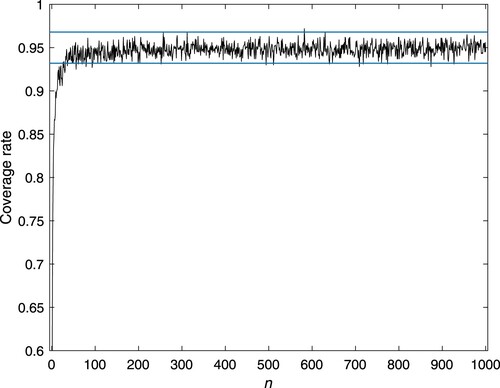$(0.95-2.576\sqrt{0.95\times 0.05/1000},0.95+2.576\sqrt{0.95\times 0.05/1000})=(0.932,0.968).$For different n, Figures 1 and 2 display the coverage rate of the 95$\mathrm{\%}$ confidence interval of the MTTF. It is observed that the coverage rate of the 95$\mathrm{\%}$ confidence interval of the MTTF basically fluctuates within the theoretical interval of (0.932, 0.968) when the sample size n is large enough.

Figure 1. Case 1: Coverage rate of the 95% confidence interval of the MTTF.

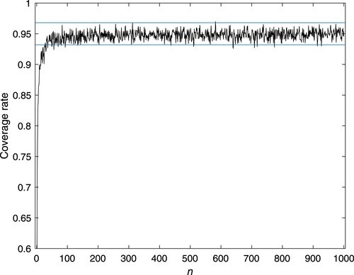
Figure 2. Case 2: Coverage rate of the 95$\mathrm{\%}$ confidence interval of the MTTF.

For different thresholds, the simulated ML and SD of the 95% confidence interval for the MTTF are given in Tables 3 and 4. In Tables 3 and 4, it is observed that the SD gradually decreases and approaches 0 as n increases. For the proposed confidence level, the interval estimation with the smallest mean length of the interval is the best. As n increases, the ML of the interval becomes progressively shorter, and the confidence interval performs better. Combining the coverage rate, ML and SD of the confidence interval, it is discovered that the simulation of the asymptotic confidence interval of the MTTF is optimistic, and the larger the sample size n, the better the result.

Table 3. Case 1: ML and SD.

n	20	30	50	100	300	500	700	1000
ML	21.1661	17.5473	13.6808	9.6781	5.6018	4.3411	3.6751	3.0714
SD	3.4699	2.1647	1.4283	0.6667	0.2193	0.1347	0.0970	0.0677

Table 4. Case 2: ML and SD.

n	20	30	50	100	300	500	700	1000
ML	23.3519	19.2591	15.0537	10.6336	6.1703	4.7861	4.0379	3.3802
SD	3.5426	2.4887	1.4983	0.7956	0.2484	0.1523	0.1102	0.0738

4.4. Power function and Type I error rate for hypothesis testing

For a given n, after constructing the asymptotic confidence interval of the MTTF, the power function is calculated by taking the significance level $\alpha =0.05$, considering ${\mathrm{MTTF}}^{\ast }=32$. In Section 4.3, and the simulations are run 1000 times, and the results are recorded as $({\widehat{\mathrm{MTTF}}}_{(1)},{\hat{\sigma }}_{(1)}^2)$, $({\widehat{\mathrm{MTTF}}}_{(2)},{\hat{\sigma }}_{(2)}^2)$, …, $({\widehat{\mathrm{MTTF}}}_{(1000)},{\hat{\sigma }}_{(1000)}^2)$. Let $I_c$ be the indicator function that the cth simulated estimation result of the MTTF falls within the rejection region, and the simulated value of the power function is $\hat{g}(\mathrm{MTTF})=\sum _{c=1}^{1000}{I}_c/1000$.

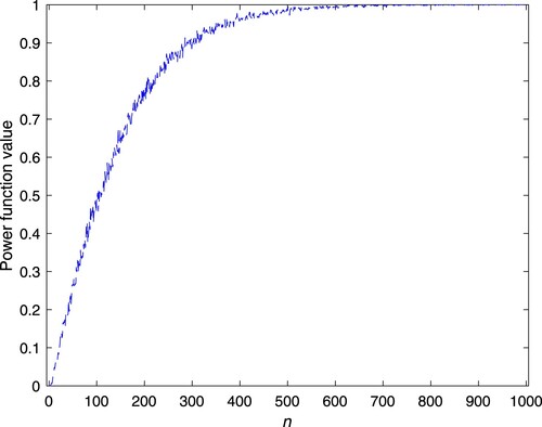
Figures 3 and 4 show the simulated power function values of the test for different sample sizes n. As can be seen, $\hat{g}(\mathrm{MTTF})$ increases as n increases for any given $\mathrm{MTTF}>{\mathrm{MTTF}}^{\ast }$ and converges to a maximum value of 1. The probability of $\widehat{\mathrm{MTTF}}$ falling within the rejection region approaches 1, which is clearly in line with the actual situation. Comparing Figures 3 and 4, it is observed that the speed of the power function value tending to 1 in Case 2 is faster than that in Case 1. In Section 4.2, the MTTF of Case 2 is larger than that of Case 1 under the same parameters. Therefore the distance between MTTF and ${\mathrm{MTTF}}^{\ast }$ is positively correlated with the speed of the power function value tending to 1.

Figure 3. Case 1: Power function value of the test.

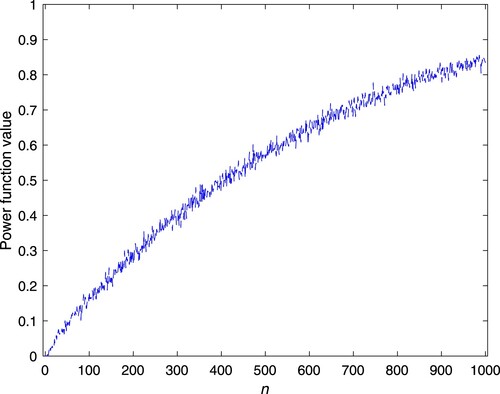
Figure 4. Case 2: Power function value of the test.

By considering the case of $\mathrm{MTTF}={\mathrm{MTTF}}^{\ast }$, Type I error rate is simulated to evaluate the performance of the rejection rule. In Cases 1 and 2, let ${\mathrm{MTTF}}^{\ast }=34.0674$ and ${\mathrm{MTTF}}^{\ast }=36.5550$, respectively. Type I error rate is the probability of $\widehat{\mathrm{MTTF}}$ falling within the rejection region when $\mathrm{MTTF}={\mathrm{MTTF}}^{\ast }$. So the simulated Type I error rate is $\hat{\alpha }(\mathrm{MTTF})=\sum _{c=1}^{1000}{I}_c/1000$. $\sum _{c=1}^{1000}{I}_c$ follows the binomial distribution B(1000, 0.05), $\frac{\sum _{c=1}^{1000}{I}_c-50}{\sqrt{1000\times 0.05\times 0.95}}=\frac{\hat{\alpha }(\mathrm{MTTF})-0.05}{\sqrt{0.05\times 0.95/1000}}\sim N(0,1),$which is obtained by the CLT. Thus, the probability of $\hat{\alpha }(\mathrm{MTTF})$ falling into the following interval is 99%. $(0.05-2.576\sqrt{0.05\times 0.95/1000},0.05+2.576\sqrt{0.05\times 0.95/1000})=(0.0322,0.0678).$

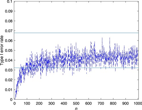
Figures 5 and 6 show the simulated Type I error rate of the test for Cases 1 and 2, respectively. It is observed that the Type I error rate basically fluctuates within the theoretical interval of (0.0322, 0.0678) when the sample size n is large enough.

Figure 5. Case 1: Type I error rate of the test.

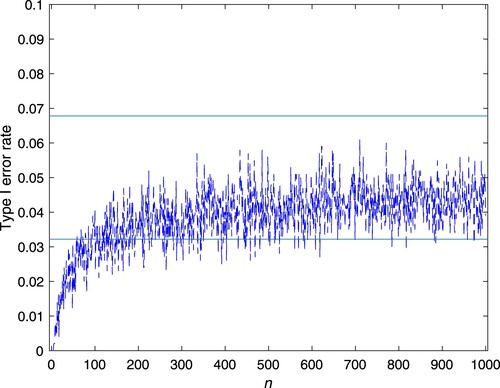
Figure 6. Case 2: Type I error rate of the test.

5. Conclusion

This work investigates a statistical inference problem about the MTTF of a K-out-of-N: G system in a shock environment, which is modeled by considering switching failure, mixed standby and Poisson shocks. Based on the Markov process theory, the state transition rate matrix of the system and state probability equations are constructed to deduce the analytical expression of the MTTF. The MLE and the asymptotic confidence interval of the MTTF are obtained by using sample data generated from random simulations. As the sample size increases, the simulation results demonstrate that the MLE of the MTTF is closer to the true value, the ML and SD of the asymptotic confidence interval gradually decrease, and the performance of the power function for the hypothesis testing becomes better. Based on the basic values of system parameters, the MTTF for two different cases of the shock threshold are compared. It is observed that the MTTF under Case 2 is larger than that under Case 1. The effect of each parameter on the MTTF is analyzed, which indicates that the component's failure rate ${\lambda }_a$ has a greater effect on the MTTF than the intensity of the shocks ${\lambda }_b$. In the system model of this paper, the lifetime of all components follows an exponential distribution. While it would be more general to study a situation where the lifetime of components follows a general distribution. Therefore, Poisson shocks and switching failure can be introduced into complex systems with general distribution in the future, which has important theoretical significance and reference value for the analysis and evaluation of system reliability index.

CRediT author statement

Fang Luo: Methodology, Software, Writing – original draft preparation, Visualization. Linmin Hu: Conceptualization, Writing – review and editing, Funding acquisition. Yuyu Wang: Writing – review and editing. Xiaoyun Yu: Validation.

Disclosure statement

No potential conflict of interest was reported by the author(s).

Additional information

Funding

This work was supported by the National Natural Science Foundation of China [grant number 72071175], the Project of Hebei Key Laboratory of Software Engineering [grant number 22567637H], and the Basic Innovative Research and Cultivation Project of Yanshan University [grant number 2023LGZD003].

References

- Ali, A., Khaliq, S., Ali, Z., & Dey, S. (2018). Reliability estimation of s-out-of-k system for non-identical stress-strength components. Life Cycle Reliability and Safety Engineering, 7(1), 33–41. https://doi.org/10.1007/s41872-018-0039-7
- Amari, S. V., & Dill, G. (2009). A new method for reliability analysis of standby systems. In 2009 Annual Reliability and Maintainability Symposium (pp. 417–422).
- Baek, S., & Jeon, G. (2013). A k-out-of-n system reliability optimization problem with mixed redundancy. Journal of the Korean Institute of Industrial Engineers, 39(2), 90–98. https://doi.org/10.7232/JKIIE.2013.39.2.090
- Barlow, R. E., & Proschan, F. (1975). Statistical theory of reliability and life testing: Probability models. Holt, Rinehart and Winston.
- Boddu, P., & Xing, L. (2012). Redundancy allocation for k-out-of-n: G systems with mixed spare types. In 2012 Proceedings Annual Reliability and Maintainability Symposium (pp. 1–6).
- Chien, Y. H., Ke, J. C., & Lee, S. L. (2006). Asymptotic confidence limits for performance measures of a repairable system with imperfect service station. Communication in Statistics-Simulation and Computation, 35(3), 813–830. https://doi.org/10.1080/03610910600716563
- El-Sherbeny, M. S., & Elshoubary, E. (2020). Stochastic analysis of reliability indices for a redundant system under Poisson shocks. International Journal of Computer Applications, 176(19), 21–30. https://doi.org/10.5120/ijca2020920143
- El-Sherbeny, M. S., & Hussien, Z. M. (2022). Reliability analysis of a two nonidentical unit parallel system with optional vacations under Poisson shocks. Mathematical Problems in Engineering, 2022, 2488182. https://doi.org/10.1155/2022/2488182
- Ge, X., Sun, J., & Wu, Q. (2021). Reliability analysis for a cold standby system under stepwise Poisson shocks. Journal of Control and Decision, 8(1), 27–40. https://doi.org/10.1080/23307706.2019.1633961
- Hsu, Y. L., Ke, J. C., & Liu, T. H. (2011). Standby system with general repair, reboot delay, switching failure and unreliable repair facility—A statistical standpoint. Mathematics and Computers in Simulation, 81(11), 2400–2413. https://doi.org/10.1016/j.matcom.2011.03.003
- Hsu, Y. L., Ke, J. C., Liu, T. H., & Wu, C. H. (2014). Modeling of multi-server repair problem with switching failure and reboot delay and related profit analysis. Computers and Industrial Engineering, 69, 21–28. https://doi.org/10.1016/j.cie.2013.12.003
- Jana, N., & Bera, S. (2022). Interval estimation of multicomponent stress-strength reliability based on inverse Weibull distribution. Mathematics and Computers in Simulation, 191, 95–119. https://doi.org/10.1016/j.matcom.2021.07.026
- Kang, J., Hu, L., Peng, R., Li, Y., & Tian, R. (2023). Availability and cost-benefit evaluation for a repairable retrial system with warm standbys and priority. Statistical Theory and Related Fields, 7(2), 164–175. https://doi.org/10.1080/24754269.2022.2152591
- Ke, J. B., Lee, W. C., & Ke, J. C. (2008). Reliability-based measure for a system with standbys subjected to switching failures. Engineering Computations, 25(7), 694–706. https://doi.org/10.1108/02644400810899979
- Ke, J. C., Chang, C. J., & Lee, W. C. (2018). An availability-based system with general repair via Bayesian aspect. Mathematics and Computers in Simulation, 144, 247–265. https://doi.org/10.1016/j.matcom.2017.09.001
- Ke, J. C., Liu, T. H., & Yang, D. Y. (2016). Machine repairing systems with standby switching failure. Computers and Industrial Engineering, 99, 223–228. https://doi.org/10.1016/j.cie.2016.07.016
- Kızılaslan, F. (2018). Classical and Bayesian estimation of reliability in a multicomponent stress–strength model based on a general class of inverse exponentiated distributions. Statistical Papers, 59(3), 1161–1192. https://doi.org/10.1007/s00362-016-0810-7
- Lewis, E. (1996). Introduction to reliability engineering (2nd ed.) John Wiley & Sons.
- Liu, T. H., Huang, Y. L., Lin, Y. B., & Chang, F. M. (2022). Cost-benefit analysis of a standby retrial system with an unreliable server and switching failure. Computation, 10(4), 48–64. https://doi.org/10.3390/computation10040048
- Patawa, R., Pundir, P. S., Sigh, A. K., & Singh, A. (2022). Some inferences on reliability measures of two-non-identical units cold standby system waiting for repair. International Journal of System Assurance Engineering Management, 13, 172–188.
- Pham, H., & Pham, M. (1991). Optimal designs of (k, n-k+1)-out-of-n: F system (subject to 2 failure modes) optimal designs of (k, n-k+1)-out-of-n: F system (subject to 2 failure modes). IEEE Transactions on Reliability, 40(5), 559–562. https://doi.org/10.1109/24.106777
- Rasekhi, M., Saber, M. M., & Yousof, H. M. (2020). Bayesian and classical inference of reliability in multicomponent stress-strength under the generalized logistic model. Communications in Statistics-Theory and Methods, 50(21), 5114–5125. https://doi.org/10.1080/03610926.2020.1726958
- Shanthikumar, J. G., & Sumita, U. (1983). General shock models associated with correlated renewal sequences. Journal of Applied Probability, 20(3), 600–614. https://doi.org/10.2307/3213896
- Shanthikumar, J. G., & Sumita, U. (1984). Distribution properties of the system failure time in a general shock model. Advances in Applied Probability, 16(2), 363–377. https://doi.org/10.2307/1427074
- She, J., & Pecht, M. G. (1992). Reliability of a k-out-of-n warm-standby system. IEEE Transactions on Reliability, 41(1), 72–75. https://doi.org/10.1109/24.126674
- Shekhar, C., Kumar, N., Gupta, A., Kumar, A., & Varshney, S. (2020). Warm-spare provisioning computing network with switching failure, common cause failure, vacation interruption, and synchronized reneging. Reliability Engineering and System Safety, 199, 106910. https://doi.org/10.1016/j.ress.2020.106910
- Wang, K. H., & Chen, Y. J. (2009). Comparative analysis of availability between three systems with general repair times, reboot delay and switching failures. Applied Mathematics and Computation, 215(1), 384–394. https://doi.org/10.1016/j.amc.2009.05.023
- Wang, L., Wu, K., Tripathi, Y. M., & Lodhi, C. (2020). Reliability analysis of multicomponent stress–strength reliability from a bathtub-shaped distribution. Journal of Applied Statistics, 49(1), 122–142. https://doi.org/10.1080/02664763.2020.1803808
- Wu, Q. (2012). Reliability analysis of a cold standby system attacked by shocks. Applied Mathematics and Computation, 218(23), 11654–11673. https://doi.org/10.1016/j.amc.2012.05.051
- Wu, Q., & Wu, S. (2011). Reliability analysis of two-unit cold standby repairable systems under Poisson shocks. Applied Mathematics and Computation, 218(1), 171–182. https://doi.org/10.1016/j.amc.2011.05.089
- Wu, Q., Zhang, J., & Tang, J. (2015). Reliability evaluation for a class of multi-unit cold standby systems under Poisson shocks. Communications in Statistics-Theory and Methods, 44(15), 3278–3288. https://doi.org/10.1080/03610926.2013.851232
- Yang, D. Y., & Wu, C. H. (2021). Evaluation of the availability and reliability of a standby repairable system incorporating imperfect switchovers and working breakdowns. Reliability Engineering and System Safety, 207, 107366. https://doi.org/10.1016/j.ress.2020.107366