Extraction of optical wave structures to the coupled fractional system in magneto-optic waveguides

Abstract

In this article, truncated M-fractional coupled nonlinear Schrodinger equation (NLSE) with quadratic–cubic nonlinearity is under observation. The studied model is composed of chromatic dispersion, magneto-optic parameter and inter-modal dispersion. The NLSE is the most significant physical model to explain the fluctuations of optical soliton proliferation. The NLSEs have become more popular because of the clarity with which they explain a wide range of complex physical phenomena and the depth with which they display dynamical patterns via localized wave solutions. Optical soliton propagation in magneto-optic is currently a subject of great interest due to the multiple prospects for ultrafast signal routing systems and short light pulses in communications. The optical solitons are secured in the forms of bright, dark, singular and combo solitons. In addition, hyperbolic, periodic and exponential function solutions have been recovered. The modified Sardar subequation and enhanced modified extended tanh-expansion approaches recently developed integration tools are adopted in this study for securing the solutions. In nonlinear dispersive media, optical solitons are stretched electromagnetic waves that maintain their intensity due to a balance between the effects of dispersion and nonlinearity. The effect of parameters have been observed by allotting suitable values and sketching the different shapes of the graphs.

Keywords:

• Enhanced modified extended tanh-expansion approach
• fractional derivative
• modified sardar subequation method
• optical solitons
• quadratic–cubic nonlinearity

1. Introduction

Soliton theory has attracted significant interest due to its importance in the domains of telecommunications, mathematical physics, engineering and various other branches of nonlinear sciences (Akinyemi, Şenol, Tasbozan, & Kurt, 2022). Recently, optical solitons in particular have been actively the interested research topic. In systems for fiber transmission, solitons may act as natural optical information bits, propagating almost insensitively to polarization mode and chromatic dispersion across large distances and maintaining their particle-like characteristics even when there are massive perturbations, hence making them the best options to utilize in all-optical switching systems (Zhao, Mathanaranjan, Rezazadeh, Akinyemi, & Inc, 2022). Mathanaranjan, Kumar, Rezazadeh, and Akinyemi (2022) and Younas, Yao, Ismael, Sulaiman, and Murad (2024) predicted the existence of solitons in nonlinear optical fibers in 1973, and their existence was experimentally verified in 1980. Since then, both experimental and theoretical physicists have been fascinated by this subject due to its numerous applications. Optical solitons can exist in a variety of systems, including optic waveguides, photonic crystal fibers, bulk materials such as photorefractive materials, and photopolymers.

NLPDEs are frequently used to model various computational, technological, and scientific problems. These models are extensively used in various fields such as astronomy, chemical analysis, biological processes, fiber studies, and flow dynamics (Altawallbeh et al., 2022; Nasreen et al., 2023). NLPDEs are mathematical models used to simulate complex natural phenomena in various fields such as development, sciences, engineering, biochemistry, and dynamics (Younas, Ren, Sulaiman, Bilal, & Yusuf, 2022). One of the prominent and extensively employed models is the NLSE, which is applicable in various scientific scenarios such as light propagation in irregular optical fibers, liquid structure, cell biology, deformable materials, atomic structure, turbulent phenomena, rotating magnetic fields, hydraulics, imaging, chemical kinetics, electricity, superconductivity, electromagnetic wave transmission, and several other fields (Mathanaranjan, 2023a,b; Mathanaranjan & Vijayakumar, 2022). Moreover, fractional form of the NLPDEs have received significant interest from researchers due to their extensive scientific applications and frequent occurrence in research and industrial settings. These mathematical representations can be utilized to illustrate various phenomena in the domains of electricity, electrochemistry, information processing, solid mechanics, physiological community models, and fluid dynamics. Currently, researchers are exploring various effective methods to handle the complex structures of physical applications that have emerged as a result of the development of conceptual computing bundles (Alshammari, Al-Sawalha, & Shah, 2023; Han, Li, & Li, 2023; Jamal, Ullah, Ahmad, Sarwar, & Shokri, 2023; Mirzazadeh, Sharif, Hashemi, Akgül, & El Din, 2023). Furthermore, in order to properly appreciate the relevance of these derivatives in a range of nonlinear physical processes, significant developments are being achieved in the definition of fractional derivatives (Alshehry, Yasmin, Ghani, Shah, & Nonlaopon, 2023; Jamal et al., 2023). Compared to the integer derivative, the fractional derivative demonstrates a broader connection and can accurately represent the dynamic processes involved in function construction. The field of fractional calculus encompasses a wide range of topics including applied mathematics, fluid mechanics, hydrodynamics, system identification, quasi-chaotic dynamical systems, statistics, finance, ecology, chaotic dynamical systems, optical fibers, solid-state biology, and electric control theory. Unlike traditional calculus, which only evaluates the present condition of the problem, the fractional derivative employed in mathematical modeling of these situations provides a logical explanation for the nonlocal characteristics of these models. Different computational techniques have been developed for analyzing the nonlinear complicated systems governed by fractional and non-fractional differential equations the in recent years. Some methods are like truncated Painlevé approach (Raza, Rani, Chahlaoui, & Shah, 2023), Riccati equation mapping method (Zhu, 2008), improved F-expansion function method (Akram, Ahmad, Rehman, & Ali, 2023), Lie symmetry technique (Raza, Rani, et al., 2023), bifurcation analysis (Han, Li, et al., 2023), modified simple equation technique (Zayed & Ibrahim, 2012), iterative transform method (Shah, Agarwa, Chung, El-Zahar, & Hamed, 2020), new sub equation method and modified Khater’s method (Tripathy, Sahoo, Rezazadeh, Izgi, & Osman, 2023), Hirota bilinear method (Younas, Ren, et al., 2022), new extended auxiliary equation method (Mathanaranjan, 2023). Every approach possesses a distinct set of prerequisites that must be fulfilled in order to be employed in the governing framework. In recent times, there has been a growing interest among researchers and analysts in obtaining exact soliton solutions for nonlinear dynamical systems. This effort is facilitated by the availability of computer tools that ease the laborious and time-consuming mathematical calculations involved in this process.

However, this study aims to uncover the optical solitons and other solutions in magneto-optic waveguides. The governing system is represented by a fractional coupled system of NLSE with quadratic-cubic nonlinearity. The solutions are obtained through a robust integration methods known as the modified Sardar sub equation (MSSE) method (Akinyemi et al., 2024; Ibrahim, Sulaiman, Yusuf, Ozsahin, & Baleanu, 2024) and enhanced modified extended tanh-expansion method (eMETEM) (Esen, Ozisik, Secer, & Bayram, 2022). The applied methods are versatile approaches applicable to a wide range of nonlinear differential equations, especially those involving second-order differentials, some types of nonlinear partial differentials and systems. Their key advantage lies in simplifying nonlinear equations, making it easier to find solutions, including exact ones. The methods provide closed-form solutions with parameters, offering flexibility for different scenarios. While not a universal solution for all nonlinear equations, it becomes particularly useful when other methods fail. The research using these methods have unveiled novel soliton solutions with applications in mathematical physics.

The article is arranged as: Section 2 consists the governing equation. Properties of fractional derivative in Section 3 and extraction of solutions are discussed Section 4, respectively. Section 5, includes the discussion and graphical view about the earned solutions, while concluding remarks is given in Section 6.

2. The governing equation

In-depth research projects have been promoted by the improvements in optical communication technologies, quantum mechanics, computer networks, the Heisenberg spin chain, plasma physics, the Bose Einstein condensation, and condensed matter physics. These projects focus on studying the dynamics of soliton propagation through fiber optics. Numerous studies have been conducted on nonlinear optical phenomena, especially after the development of ultrashort pulse lasers. These lasers utilize the NLSE equation to simulate optical phenomena in extremely nonlinear media. The presence of soliton clutter poses a significant barrier to the propagation of solitons in optical waveguides. To overcome this effect, a favorable approach is to incorporate magneto-optic waveguides. These waveguides efficiently and beneficially transition from a state of disorder to a state of separateness. This allows for the continuous transmission of solitons, effectively resolving the issue of optical soliton collisions within the optical solitons. The M fractional form coupled NLSE in magneto-optic waveguides (Asma et al., 2020) where the QC nonlinearity is given as: (1) $$\{\begin{array}{c}i{D}_{M,t}^{ϵ,\beta }p+a_1{D}_{M,x}^{2ϵ,\beta }p+(b_1|p|+c_1|p{|}^2+d_1\left|q\right|+e_1|q{|}^2)p=\hfill \\ f_{1}q+i[{\sigma }_1{D}_{M,x}^{ϵ,\beta }p+{\lambda }_1{D}_{M,x}^{ϵ,\beta }(|p{|}^{2}p)+{\gamma }_{1}p{D}_{M,x}^{ϵ,\beta }(|p{|}^2)+{\delta }_1|p{|}^2{D}_{M,x}^{ϵ,\beta }p],\hfill \\ i{D}_{M,t}^{ϵ,\beta }q+a_2{D}_{M,x}^{2ϵ,\beta }q+(b_2|q|+c_2|q{|}^2+d_2\left|p\right|+e_2|p{|}^2)q=\hfill \\ f_{2}p+i[{\sigma }_2{D}_{M,x}^{ϵ,\beta }q+{\lambda }_2{D}_{M,x}^{ϵ,\beta }(|q{|}^{2}q)+{\gamma }_{2}q{D}_{M,x}^{ϵ,\beta }(|q{|}^2)+{\delta }_2|q{|}^2{D}_{M,x}^{ϵ,\beta }q],\hfill \end{array}$$(1) where, $a_l,$ $b_l,$ $c_l,$ $d_l,$ $e_l,$ $f_l,$ ${\sigma }_l,$ ${\gamma }_l,$ ${\lambda }_l,$ and ${\delta }_l,$ $(l=1,2)$ are constants and $i=\sqrt{-1},$ while $D_M^{ϵ,\beta }$ serves to denote the M-truncated derivative with $ϵ\in (0,1]$ and $\beta >0.$ The system (1)(1) $$\{\begin{array}{c}i{D}_{M,t}^{ϵ,\beta }p+a_1{D}_{M,x}^{2ϵ,\beta }p+(b_1|p|+c_1|p{|}^2+d_1\left|q\right|+e_1|q{|}^2)p=\hfill \\ f_{1}q+i[{\sigma }_1{D}_{M,x}^{ϵ,\beta }p+{\lambda }_1{D}_{M,x}^{ϵ,\beta }(|p{|}^{2}p)+{\gamma }_{1}p{D}_{M,x}^{ϵ,\beta }(|p{|}^2)+{\delta }_1|p{|}^2{D}_{M,x}^{ϵ,\beta }p],\hfill \\ i{D}_{M,t}^{ϵ,\beta }q+a_2{D}_{M,x}^{2ϵ,\beta }q+(b_2|q|+c_2|q{|}^2+d_2\left|p\right|+e_2|p{|}^2)q=\hfill \\ f_{2}p+i[{\sigma }_2{D}_{M,x}^{ϵ,\beta }q+{\lambda }_2{D}_{M,x}^{ϵ,\beta }(|q{|}^{2}q)+{\gamma }_{2}q{D}_{M,x}^{ϵ,\beta }(|q{|}^2)+{\delta }_2|q{|}^2{D}_{M,x}^{ϵ,\beta }q],\hfill \end{array}$$(1) is the M-fractional NLSE which propagates the optical pulses through magneto–optic waveguides with x and t that are spatial and temporal components, respectively. Here $a_l$ is coefficient chromatic dispersion (CD), $f_1$ denote the magneto-optic parameter whereas ${\sigma }_l$ represent inter-modal dispersion (IMD). The self-steepening term that prevents shock waves formation is denoted by the symbol ${\lambda }_l.$ Moreover, ${\gamma }_l$ and ${\delta }_l$ accounts for nonlinear dispersion. Now, in the next section, we recover the different forms of solutions to the studied model.

3. The truncated M-fractional derivative

Research related to solitary wave solutions is a prominent field of study, wherein the application of truncated M-fractional derivative has received significant attention from researchers. Comparing the truncated M-fractional derivative to other fractional derivatives, several recent studies have shown that it provides a more realistic representation of the behavior of solitary waves in particular nonlinear systems. Moreover, this phenomenon exhibits a wide range of applications across many disciplines in the realms of engineering and other related science, encompassing fluid dynamics, signal processing, and electro-magnetics, and others. The truncated M-fractional derivative possesses considerable importance due to its capacity to accurately depict complex systems with nonlinear dynamics, memory effects, and long-range and nonlocal interactions. This specific type of derivative equips academics and professionals with an effective tool to understand and analyze an extensive variety of physical, biological, and engineering related systems. The depiction of solitary waves is accomplished by using the truncated M-fractional derivative, that can be described as localized disturbances propagating through a medium without altering its shape. This specific derivative allows memory effects to be included in the model, hence enhancing its ability to accurately represent the dynamics of the system.

Definition 3.1.

Let $\Psi :[0,\infty )\to \mathbb{R},$ then the new truncated M -fractional derivative of h of order $\mu$ is discussed (Sousa & Oliveira, 2018) as: (2) $$\begin{array}{c}{\mathcal{D}}_M^{\sigma ,\zeta }\{(\psi )(t)\}=\underset{ϵ\to 0}{\mathrm{\text{lim}}}\frac{\psi (t{\mathbb{E}}_{\zeta }(ϵt^{1-\sigma }))-\psi (t)}{ϵ},\zeta >0,\sigma \in (0,1),\forall t>0,\hfill \end{array}$$(2) with ${\mathbb{E}}_{\zeta }(.)$ being the one parameter truncated Mittag–Leffler function (Sousa & Oliveira, 2018).

Theorem 3.1.

Let $\zeta >0,$ $0<\sigma \le 1,$ $p,s\in \mathbb{R}$, and $\psi ,\varphi$ $\mu$-differentiable at a point $t>0$. Then:

1. ${\mathcal{D}}_M^{\sigma ,\zeta }\{(p\varphi +s\psi )(t)\}=p{\mathcal{D}}_M^{\sigma ,\zeta }\{\varphi (t)\}+s{\mathcal{D}}_M^{\sigma ,\zeta }\{\psi (t)\}.$

2. ${\mathcal{D}}_M^{\sigma ,\zeta }\{(\varphi .\psi )(t)\}=\varphi (t){\mathcal{D}}_M^{\sigma ,\zeta }\{\Psi (t)\}+\psi (t){\mathcal{D}}_M^{\sigma ,\zeta }\{\varphi (t)\}.$

3. ${\mathcal{D}}_M^{\sigma ,\zeta }\{\frac{\varphi }{\psi }(t)\}=\frac{\psi (t){\mathcal{D}}_M^{\sigma ,\zeta }\{\varphi (t)\}-\varphi (t){\mathcal{D}}_M^{\sigma ,\zeta }\{\psi (t)\}}{{[\psi (t)]}^2}.$

4. ${\mathcal{D}}_M^{\sigma ,\zeta }\left\{c\right\}=0,$ where $\varphi (t)=c$ is a constant.

5. If $\varphi$ is differentiable, then ${\mathcal{D}}_M^{\sigma ,\zeta }\{\varphi (t)\}=\frac{t^{1-\sigma }}{\Gamma (\zeta +1)}\frac{d\varphi (t)}{\mathit{\text{dt}}}.$

4. Extraction of solutions

For securing a variety of solutions to Eq. (1)(1) $$\{\begin{array}{c}i{D}_{M,t}^{ϵ,\beta }p+a_1{D}_{M,x}^{2ϵ,\beta }p+(b_1|p|+c_1|p{|}^2+d_1\left|q\right|+e_1|q{|}^2)p=\hfill \\ f_{1}q+i[{\sigma }_1{D}_{M,x}^{ϵ,\beta }p+{\lambda }_1{D}_{M,x}^{ϵ,\beta }(|p{|}^{2}p)+{\gamma }_{1}p{D}_{M,x}^{ϵ,\beta }(|p{|}^2)+{\delta }_1|p{|}^2{D}_{M,x}^{ϵ,\beta }p],\hfill \\ i{D}_{M,t}^{ϵ,\beta }q+a_2{D}_{M,x}^{2ϵ,\beta }q+(b_2|q|+c_2|q{|}^2+d_2\left|p\right|+e_2|p{|}^2)q=\hfill \\ f_{2}p+i[{\sigma }_2{D}_{M,x}^{ϵ,\beta }q+{\lambda }_2{D}_{M,x}^{ϵ,\beta }(|q{|}^{2}q)+{\gamma }_{2}q{D}_{M,x}^{ϵ,\beta }(|q{|}^2)+{\delta }_2|q{|}^2{D}_{M,x}^{ϵ,\beta }q],\hfill \end{array}$$(1) , we take the transformation defined as: (3) $$\begin{array}{cc}p(x,t)\hfill & ={\Delta }_1(\eta )e^{i\psi },\hfill \\ q(x,t)\hfill & ={\Delta }_2(\eta )e^{i\psi },\hfill \\ \text{where,} \eta \hfill & =\frac{\Gamma (\beta +1)\left(x^{ϵ}-\rho t^{ϵ}\right)}{ϵ} \text{and} \psi =\frac{\Gamma (\beta +1)\left(\omega t^{ϵ}+\phi -\kappa x^{ϵ}\right)}{ϵ},\hfill \end{array}$$(3) and k, $\omega ,$ $\rho ,$ and $\phi$ represent the frequency, wave number, velocity, and phase constant, respectively, while ${\Delta }_1,{\Delta }_2$ and $\psi (x,t)$ are real-valued functions that represent the soliton’s phase component and amplitude portion, respectively. On solving Eq. (3)(3) $$\begin{array}{cc}p(x,t)\hfill & ={\Delta }_1(\eta )e^{i\psi },\hfill \\ q(x,t)\hfill & ={\Delta }_2(\eta )e^{i\psi },\hfill \\ \text{where,} \eta \hfill & =\frac{\Gamma (\beta +1)\left(x^{ϵ}-\rho t^{ϵ}\right)}{ϵ} \text{and} \psi =\frac{\Gamma (\beta +1)\left(\omega t^{ϵ}+\phi -\kappa x^{ϵ}\right)}{ϵ},\hfill \end{array}$$(3) and Eq. (1)(1) $$\{\begin{array}{c}i{D}_{M,t}^{ϵ,\beta }p+a_1{D}_{M,x}^{2ϵ,\beta }p+(b_1|p|+c_1|p{|}^2+d_1\left|q\right|+e_1|q{|}^2)p=\hfill \\ f_{1}q+i[{\sigma }_1{D}_{M,x}^{ϵ,\beta }p+{\lambda }_1{D}_{M,x}^{ϵ,\beta }(|p{|}^{2}p)+{\gamma }_{1}p{D}_{M,x}^{ϵ,\beta }(|p{|}^2)+{\delta }_1|p{|}^2{D}_{M,x}^{ϵ,\beta }p],\hfill \\ i{D}_{M,t}^{ϵ,\beta }q+a_2{D}_{M,x}^{2ϵ,\beta }q+(b_2|q|+c_2|q{|}^2+d_2\left|p\right|+e_2|p{|}^2)q=\hfill \\ f_{2}p+i[{\sigma }_2{D}_{M,x}^{ϵ,\beta }q+{\lambda }_2{D}_{M,x}^{ϵ,\beta }(|q{|}^{2}q)+{\gamma }_{2}q{D}_{M,x}^{ϵ,\beta }(|q{|}^2)+{\delta }_2|q{|}^2{D}_{M,x}^{ϵ,\beta }q],\hfill \end{array}$$(1) , we get

Real part

(4) $$\{\begin{array}{c}{a}_1{\Delta }_1^{″}-(k({\lambda }_1+{\delta }_1)-c_1){\Delta }_1^3+b_1{\Delta }_1^2-(\omega +a_1{k}^2+k{\sigma }_1){\Delta }_1+d_1{\Delta }_1{\Delta }_2+e_1{\Delta }_1{\Delta }_2^2-f_1{\Delta }_2=0,\hfill \\ a_2{\Delta }_2^{″}-(k({\lambda }_2+{\delta }_2)-c_2){\Delta }_2^3+b_2{\Delta }_2^2-(\omega +a_2{k}^2+k{\sigma }_2){\Delta }_2+d_2{\Delta }_2{\Delta }_1+e_2{\Delta }_2{\Delta }_1^2-f_2{\Delta }_1=0,\hfill \end{array}$$(4)

Imaginary part

(5) $$\begin{array}{c}\{\begin{array}{c}(\rho +2a_{1}k+{\sigma }_1){\Delta }_1^{\prime }+(3{\lambda }_1+2{\gamma }_1+{\delta }_1){\Delta }_1^2{\Delta }_1^{\prime }=0,\hfill \\ (\rho +2a_{2}k+{\sigma }_2){\Delta }_2^{\prime }+(3{\lambda }_2+2{\gamma }_2+{\delta }_2){\Delta }_2^2{\Delta }_2^{\prime }=0.\hfill \end{array}\hfill \end{array}$$(5)

Integrating Eq. (5)(5) $$\begin{array}{c}\{\begin{array}{c}(\rho +2a_{1}k+{\sigma }_1){\Delta }_1^{\prime }+(3{\lambda }_1+2{\gamma }_1+{\delta }_1){\Delta }_1^2{\Delta }_1^{\prime }=0,\hfill \\ (\rho +2a_{2}k+{\sigma }_2){\Delta }_2^{\prime }+(3{\lambda }_2+2{\gamma }_2+{\delta }_2){\Delta }_2^2{\Delta }_2^{\prime }=0.\hfill \end{array}\hfill \end{array}$$(5) by considering the zero integration constant offers (6) $$\begin{array}{c}(\rho +2a_{1}k+{\sigma }_1)H_1+(3{\lambda }_1+2{\gamma }_1+{\delta }_1)H_1^3=0,\hfill \end{array}$$(6) and (7) $$\begin{array}{c}(\rho +2a_{2}k+{\sigma }_2)H_2+(3{\lambda }_2+2{\gamma }_2+{\delta }_2)H_2^3=0,\hfill \end{array}$$(7)

Equations (6)(6) $$\begin{array}{c}(\rho +2a_{1}k+{\sigma }_1)H_1+(3{\lambda }_1+2{\gamma }_1+{\delta }_1)H_1^3=0,\hfill \end{array}$$(6) and (7)(7) $$\begin{array}{c}(\rho +2a_{2}k+{\sigma }_2)H_2+(3{\lambda }_2+2{\gamma }_2+{\delta }_2)H_2^3=0,\hfill \end{array}$$(7) provide (8) $$\begin{array}{c}\rho =-(2a_{1}k+{\sigma }_1),\hfill \end{array}$$(8) (9) $$\begin{array}{c}3{\lambda }_1+2{\gamma }_1+{\delta }_1=0,\hfill \end{array}$$(9) and (10) $$\begin{array}{c}\rho =-(2a_{2}k+{\sigma }_2),\hfill \end{array}$$(10) (11) $$\begin{array}{c}3{\lambda }_2+2{\gamma }_2+{\delta }_2=0.\hfill \end{array}$$(11)

Next, on manipulating Eqs. (8)(8) $$\begin{array}{c}\rho =-(2a_{1}k+{\sigma }_1),\hfill \end{array}$$(8) and (10)(10) $$\begin{array}{c}\rho =-(2a_{2}k+{\sigma }_2),\hfill \end{array}$$(10) , the frequency of soliton is expressed as: (12) $$\begin{array}{c}k=\frac{{\sigma }_2-{\sigma }_1}{2(a_1-a_2)},\hfill \end{array}$$(12) provided $a_1\ne a_2$ and ${\sigma }_1\ne {\sigma }_2.$ On setting: (13) $${\Delta }_2(\eta )=\zeta {\Delta }_1(\eta ),\text{with}\zeta \ne 0\text{ and }\zeta \ne 1.$$(13)

Equation (4)(4) $$\{\begin{array}{c}{a}_1{\Delta }_1^{″}-(k({\lambda }_1+{\delta }_1)-c_1){\Delta }_1^3+b_1{\Delta }_1^2-(\omega +a_1{k}^2+k{\sigma }_1){\Delta }_1+d_1{\Delta }_1{\Delta }_2+e_1{\Delta }_1{\Delta }_2^2-f_1{\Delta }_2=0,\hfill \\ a_2{\Delta }_2^{″}-(k({\lambda }_2+{\delta }_2)-c_2){\Delta }_2^3+b_2{\Delta }_2^2-(\omega +a_2{k}^2+k{\sigma }_2){\Delta }_2+d_2{\Delta }_2{\Delta }_1+e_2{\Delta }_2{\Delta }_1^2-f_2{\Delta }_1=0,\hfill \end{array}$$(4) is written as: (14) $$\begin{array}{c}\{\begin{array}{c}{a}_1{\Delta }_1^{″}-(k({\lambda }_1+{\delta }_1)-c_1-{\zeta }^2{e}_1){\Delta }_1^3+(b_1+\zeta d_1){\Delta }_1^2-(\omega +a_1{k}^2+k{\sigma }_1+\zeta f_1){\Delta }_1=0,\hfill \\ a_2\zeta {\Delta }_1^{″}-\zeta ({\zeta }^2(k{\lambda }_2+k{\delta }_2)-c_2)-e_2){\Delta }_1^3+\zeta (b_2+\zeta d_2){\Delta }_1^2-(\zeta (\omega +a_2{k}^2+k{\sigma }_2)+f_2){\Delta }_1=0.\hfill \end{array}\hfill \end{array}$$(14)

Equation (14)(14) $$\begin{array}{c}\{\begin{array}{c}{a}_1{\Delta }_1^{″}-(k({\lambda }_1+{\delta }_1)-c_1-{\zeta }^2{e}_1){\Delta }_1^3+(b_1+\zeta d_1){\Delta }_1^2-(\omega +a_1{k}^2+k{\sigma }_1+\zeta f_1){\Delta }_1=0,\hfill \\ a_2\zeta {\Delta }_1^{″}-\zeta ({\zeta }^2(k{\lambda }_2+k{\delta }_2)-c_2)-e_2){\Delta }_1^3+\zeta (b_2+\zeta d_2){\Delta }_1^2-(\zeta (\omega +a_2{k}^2+k{\sigma }_2)+f_2){\Delta }_1=0.\hfill \end{array}\hfill \end{array}$$(14) has the same form under the constraint conditions: (15) $$\begin{array}{c}\{\begin{array}{c}{a}_1=a_2\zeta .\hfill \\ b_1+\zeta d_1=\zeta (\zeta b_2+d_2).\hfill \\ \omega +a_1{k}^2+k{\sigma }_1+\zeta f_1=\zeta (\omega +a_2{k}^2+k{\sigma }_2)+f_2.\hfill \\ (k({\lambda }_1+{\delta }_1)-c_1-{\zeta }^2{e}_1=\zeta ({\zeta }^{2}k{\lambda }_2+k{\delta }_2)-c_2)-e_2).\hfill \end{array}\hfill \end{array}$$(15)

From Eq. (15)(15) $$\begin{array}{c}\{\begin{array}{c}{a}_1=a_2\zeta .\hfill \\ b_1+\zeta d_1=\zeta (\zeta b_2+d_2).\hfill \\ \omega +a_1{k}^2+k{\sigma }_1+\zeta f_1=\zeta (\omega +a_2{k}^2+k{\sigma }_2)+f_2.\hfill \\ (k({\lambda }_1+{\delta }_1)-c_1-{\zeta }^2{e}_1=\zeta ({\zeta }^{2}k{\lambda }_2+k{\delta }_2)-c_2)-e_2).\hfill \end{array}\hfill \end{array}$$(15) , $\omega$ representing the wave number can be written as (16) $$\begin{array}{c}\omega =\frac{k^2(a_1+\zeta a_2)+k(\zeta {\sigma }_2-{\sigma }_1)+f_2-\zeta f_1}{1-\zeta },\hfill \end{array}$$(16)

Equation (14)(14) $$\begin{array}{c}\{\begin{array}{c}{a}_1{\Delta }_1^{″}-(k({\lambda }_1+{\delta }_1)-c_1-{\zeta }^2{e}_1){\Delta }_1^3+(b_1+\zeta d_1){\Delta }_1^2-(\omega +a_1{k}^2+k{\sigma }_1+\zeta f_1){\Delta }_1=0,\hfill \\ a_2\zeta {\Delta }_1^{″}-\zeta ({\zeta }^2(k{\lambda }_2+k{\delta }_2)-c_2)-e_2){\Delta }_1^3+\zeta (b_2+\zeta d_2){\Delta }_1^2-(\zeta (\omega +a_2{k}^2+k{\sigma }_2)+f_2){\Delta }_1=0.\hfill \end{array}\hfill \end{array}$$(14) may be rewrite as (17) $$\begin{array}{c}{\Delta }_1^{″}-{\Gamma }_1{\Delta }_1^3+{\Gamma }_2{\Delta }_1^2-{\Gamma }_3{\Delta }_1^3=0,\hfill \end{array}$$(17) where, ${\Gamma }_1=\frac{(k({\lambda }_1+{\delta }_1)-c_1-{\zeta }^2{e}_1)}{a_1},$ ${\Gamma }_2=\frac{b_1+\zeta d_1}{a_1},$ and ${\Gamma }_3=\frac{(\omega +a_1{k}^2+k{\sigma }_1+\zeta f_1)}{a_1}.$ Next, on making the balance between ${\Delta }_1^{″}$ and ${\Delta }_1^3$ in above equation gives $n=1.$

4.1. Solutions via modified sardar subequation method

Based on $n=1,$ we apply the proposed method to secure the solutions. The general form of the solution for MSSE method (Ibrahim et al., 2024) is expressed as: (18) $$\begin{array}{c}\begin{array}{c}{\Delta }_1(\eta )={\varphi }_0+\sum _{r=1}^n{\varphi }_r{\Theta }^r(\eta ),\hfill \end{array}\hfill \end{array}$$(18)

For $n=1,$ the above solution takes the form as: (19) $$\begin{array}{c}{\Delta }_1(\eta )={\varphi }_0+{\varphi }_1\Theta (\eta ).\hfill \end{array}$$(19)

On putting Eq. (19)(19) $$\begin{array}{c}{\Delta }_1(\eta )={\varphi }_0+{\varphi }_1\Theta (\eta ).\hfill \end{array}$$(19) in Eq. (17)(17) $$\begin{array}{c}{\Delta }_1^{″}-{\Gamma }_1{\Delta }_1^3+{\Gamma }_2{\Delta }_1^2-{\Gamma }_3{\Delta }_1^3=0,\hfill \end{array}$$(17) , we get

Set 1 ${\varphi }_0=-\frac{3{\phi }_1}{{\Gamma }_2},{\varphi }_1=\frac{3i\sqrt{2}\sqrt{{\phi }_1}\sqrt{{\phi }_2}}{{\Gamma }_2},{\Gamma }_1=-\frac{{\Gamma }_2^2}{9{\phi }_1},{\Gamma }_3=-2{\phi }_1.$

Set 2 ${\varphi }_0=-\frac{i\sqrt{{\phi }_1}}{\sqrt{{\Gamma }_1}},{\varphi }_1=-\frac{\sqrt{2}\sqrt{{\phi }_2}}{\sqrt{{\Gamma }_1}},{\Gamma }_3=-2{\phi }_1,{\Gamma }_2=-3i\sqrt{{\Gamma }_1}\sqrt{{\phi }_1}.$

For set 1, the following solutions are secured as:

(I): When ${\phi }_0=0,$ ${\phi }_1>0$ and ${\phi }_2\ne 0,$ we have

The bright soliton solution (20) $$\begin{array}{l}{p}_1(x,t)=-\frac{3\hspace{0.17em}\mathrm{\text{exp}}\hspace{0.17em}\left(\frac{i\Gamma (\beta +1)\left(\frac{t^{ϵ}\left({\kappa }^2\left(a_1+\zeta {\mathrm{a}}_2\right)+f_2-\zeta {\mathrm{f}}_1+\kappa \left(\zeta {\sigma }_2-{\sigma }_1\right)\right)}{1-\frac{\Gamma (\beta +1)\left(x^{ϵ}-\rho t^{ϵ}\right)}{ϵ}}+\phi -\kappa x^{ϵ}\right)}{ϵ}\right)}{{\Gamma }_2}\\ \times \left({\phi }_1-i\sqrt{2}\sqrt{{\phi }_1}\sqrt{-\frac{{\phi }_1}{{\phi }_2}}\sqrt{{\phi }_2}\text{sech}\left(\sqrt{{\phi }_1}\left(\frac{\Gamma (\beta +1)\left(x^{ϵ}-\rho t^{ϵ}\right)}{ϵ}+\vartheta \right)\right)\right).\end{array}$$(20)

The explicit solitary wave solution (21) $$\begin{array}{l}{p}_2(x,t)=-\frac{3\hspace{0.17em}\mathrm{\text{exp}}\hspace{0.17em}\left(\frac{i\Gamma (\beta +1)\left(\frac{ϵt^{ϵ}\left(\kappa \left(\kappa \left(a_1+\zeta {\mathrm{a}}_2\right)+\zeta {\sigma }_2-{\sigma }_1\right)+f_2-\zeta {\mathrm{f}}_1\right)}{\Gamma (\beta +1)\left(\rho t^{ϵ}-x^{ϵ}\right)+ϵ}+\phi -\kappa x^{ϵ}\right)}{ϵ}\right)}{{\Gamma }_2}\\ \times \left(\sqrt{{\phi }_1}-i\sqrt{2}\sqrt{\frac{{\phi }_1}{{\phi }_2}}\sqrt{{\phi }_2}\text{csch}\left(\sqrt{{\phi }_1}\left(\frac{\Gamma (\beta +1)\left(x^{ϵ}-\rho t^{ϵ}\right)}{ϵ}+\vartheta \right)\right)\right).\end{array}$$(21)

(II): When ${\phi }_2=\pm 4{\beta }_1{\beta }_2,$ ${\phi }_0=0$ and ${\phi }_1>0,$ where ${\beta }_1,$ ${\beta }_2$ are nonzero constants, we get (22) $$\begin{array}{l}{p}_3(x,t)=\frac{3\hspace{0.17em}\mathrm{\text{exp}}\hspace{0.17em}\left(\frac{i\Gamma (\beta +1)\left(\frac{ϵt^{ϵ}\left(\kappa \left(\kappa \left(a_1+\zeta {\mathrm{a}}_2\right)+\zeta {\sigma }_2-{\sigma }_1\right)+f_2-\zeta {\mathrm{f}}_1\right)}{\Gamma (\beta +1)\left(\rho t^{ϵ}-x^{ϵ}\right)+ϵ}+\phi -\kappa x^{ϵ}\right)}{ϵ}\right)}{{\Gamma }_2}\\ \times \left(-1+\frac{2i\sqrt{2}\sqrt{{\beta }_1{\beta }_2}{e}^{\sqrt{{\phi }_1}\left(\frac{\Gamma (\beta +1)\left(x^{ϵ}-\rho t^{ϵ}\right)}{ϵ}+\vartheta \right)}}{{\beta }_1{e}^{2\sqrt{{\phi }_1}\left(\frac{\Gamma (\beta +1)\left(x^{ϵ}-\rho t^{ϵ}\right)}{ϵ}+\vartheta \right)}-{\beta }_2}\right){\phi }_1.\end{array}$$(22)

(III): When ${\phi }_0=\frac{{\phi }_1^2}{4{\phi }_2},{\phi }_1<0,{\phi }_2>0,$ we have

The dark soliton solution (23) $$\begin{array}{l}{p}_4(x,t)=-\frac{3\hspace{0.17em}\mathrm{\text{exp}}\hspace{0.17em}\left(\frac{i\Gamma (\beta +1)\left(\frac{ϵt^{ϵ}\left(a_1{\kappa }^2+f_2+\zeta {\mathrm{a}}_2{\kappa }^2-\zeta {\mathrm{f}}_1+\zeta {\sigma }_2\kappa -\kappa {\sigma }_1\right)}{\Gamma (\beta +1)\left(\rho t^{ϵ}-x^{ϵ}\right)+ϵ}+\phi -\kappa x^{ϵ}\right)}{ϵ}\right)}{{\Gamma }_2}\\ \times \left(\sqrt{{\phi }_1}\left(\sqrt{{\phi }_1}-i\sqrt{-\frac{{\phi }_1}{{\phi }_2}}\sqrt{{\phi }_2}\mathrm{\text{tanh}}\left(\frac{\sqrt{-{\phi }_1}\left(\frac{\Gamma (\beta +1)\left(x^{ϵ}-\rho t^{ϵ}\right)}{ϵ}+\vartheta \right)}{\sqrt{2}}\right)\right)\right).\end{array}$$(23)

The singular soliton solution (24) $$\begin{array}{l}{p}_5(x,t)=-\frac{3\hspace{0.17em}\mathrm{\text{exp}}\hspace{0.17em}\left(\frac{i\Gamma (\beta +1)\left(\frac{ϵt^{ϵ}\left(a_1{\kappa }^2+f_2+\zeta {\mathrm{a}}_2{\kappa }^2-\zeta {\mathrm{f}}_1+\zeta {\sigma }_2\kappa -\kappa {\sigma }_1\right)}{\Gamma (\beta +1)\left(\rho t^{ϵ}-x^{ϵ}\right)+ϵ}+\phi -\kappa x^{ϵ}\right)}{ϵ}\right)}{{\Gamma }_2}\\ \times \left(\sqrt{{\phi }_1}\left(\sqrt{{\phi }_1}-i\sqrt{-\frac{{\phi }_1}{{\phi }_2}}\sqrt{{\phi }_2}\mathrm{\text{coth}}\left(\frac{\sqrt{-{\phi }_1}\left(\frac{\Gamma (\beta +1)\left(x^{ϵ}-\rho t^{ϵ}\right)}{ϵ}+\vartheta \right)}{\sqrt{2}}\right)\right)\right).\end{array}$$(24)

The combo bright-dark soliton solution (25) $$\begin{array}{l}{p}_6(x,t)=-\frac{3\hspace{0.17em}\mathrm{\text{exp}}\hspace{0.17em}\left(\frac{i\Gamma (\beta +1)\left(\frac{ϵt^{ϵ}\left(a_1{\kappa }^2+f_2+\zeta {\mathrm{a}}_2{\kappa }^2-\zeta {\mathrm{f}}_1+\zeta {\sigma }_2\kappa -\kappa {\sigma }_1\right)}{\Gamma (\beta +1)\left(\rho t^{ϵ}-x^{ϵ}\right)+ϵ}+\phi -\kappa x^{ϵ}\right)}{ϵ}\right)}{{\Gamma }_2}\\ \times \sqrt{{\phi }_1}(\sqrt{{\phi }_1}-\sqrt{-\frac{{\phi }_1}{{\phi }_2}}\sqrt{{\phi }_2}(\text{sech}\left(\sqrt{2}\sqrt{-{\phi }_1}\left(\frac{\Gamma (\beta +1)\left(x^{ϵ}-\rho t^{ϵ}\right)}{ϵ}+\vartheta \right)\right)\\ +i\mathrm{\text{tanh}}\left(\sqrt{2}\sqrt{-{\phi }_1}\left(\frac{\Gamma (\beta +1)\left(x^{ϵ}-\rho t^{ϵ}\right)}{ϵ}+\vartheta \right)\right))).\end{array}$$(25)

The solitary wave solutions (26) $$\begin{array}{l}{p}_7(x,t)=\hspace{0.17em}\mathrm{\text{exp}}\hspace{0.17em}\left(\frac{i\Gamma (\beta +1)\left(\frac{ϵt^{ϵ}\left(a_1{\kappa }^2+f_2+\zeta {\mathrm{a}}_2{\kappa }^2-\zeta {\mathrm{f}}_1+\zeta {\sigma }_2\kappa -\kappa {\sigma }_1\right)}{\Gamma (\beta +1)\left(\rho t^{ϵ}-x^{ϵ}\right)+ϵ}+\phi -\kappa x^{ϵ}\right)}{ϵ}\right)\\ \times \left(-\frac{3{\phi }_1}{{\Gamma }_2}+\frac{3i\sqrt{{\phi }_1}\sqrt{-\frac{{\phi }_1}{{\phi }_2}}\sqrt{{\phi }_2}\left(\mathrm{\text{coth}}\left(\frac{\sqrt{-{\phi }_1}\left(\frac{\Gamma (\beta +1)\left(x^{ϵ}-\rho t^{ϵ}\right)}{ϵ}+\vartheta \right)}{2\sqrt{2}}\right)+\mathrm{\text{tanh}}\left(\frac{\sqrt{-{\phi }_1}\left(\frac{\Gamma (\beta +1)\left(x^{ϵ}-\rho t^{ϵ}\right)}{ϵ}+\vartheta \right)}{2\sqrt{2}}\right)\right)}{2{\Gamma }_2}\right).\end{array}$$(26) (27) $$\begin{array}{l}{p}_8(x,t)=\frac{\hspace{0.17em}\mathrm{\text{exp}}\hspace{0.17em}\left(\frac{i\Gamma (\beta +1)\left(\frac{ϵt^{ϵ}\left(a_1{\kappa }^2+f_2+\zeta {\mathrm{a}}_2{\kappa }^2-\zeta {\mathrm{f}}_1+\zeta {\sigma }_2\kappa -\kappa {\sigma }_1\right)}{\Gamma (\beta +1)\left(\rho t^{ϵ}-x^{ϵ}\right)+ϵ}+\phi -\kappa x^{ϵ}\right)}{ϵ}\right)}{{\Gamma }_2} \\ \times (-3{\phi }_1-\frac{3i\sqrt{{\phi }_1}\sqrt{-\frac{{\phi }_1}{{\phi }_2}}\sqrt{{\phi }_2}\mathrm{\text{cosh}}\left(\sqrt{2}\sqrt{-{\phi }_1}\left(\frac{\Gamma (\beta +1)\left(x^{ϵ}-\rho t^{ϵ}\right)}{ϵ}+\vartheta \right)\right)}{\mathrm{\text{sinh}}\left(\sqrt{2}\sqrt{-{\phi }_1}\left(\frac{\Gamma (\beta +1)\left(x^{ϵ}-\rho t^{ϵ}\right)}{ϵ}+\vartheta \right)\right)-i}).\end{array}$$(27)

For set 2, the following solutions are extracted as:

(IV): When ${\phi }_0=0,$ ${\phi }_1<0$ and ${\phi }_2\ne 0,$ we have (28) $$\begin{array}{l}{p}_9(x,t)=\frac{\hspace{0.17em}\mathrm{\text{exp}}\hspace{0.17em}\left(\frac{i\Gamma (\beta +1)\left(\frac{ϵt^{ϵ}\left(a_1{\kappa }^2+f_2+\zeta {\mathrm{a}}_2{\kappa }^2-\zeta {\mathrm{f}}_1+\zeta {\sigma }_2\kappa -\kappa {\sigma }_1\right)}{\Gamma (\beta +1)\left(\rho t^{ϵ}-x^{ϵ}\right)+ϵ}+\phi -\kappa x^{ϵ}\right)}{ϵ}\right)}{\sqrt{{\Gamma }_1}} \\ \times \left(\sqrt{2}\sqrt{-\frac{{\phi }_1}{{\phi }_2}}\sqrt{{\phi }_2}\hspace{0.17em}\text{sec}\hspace{0.17em}\left(\sqrt{-{\phi }_1}\left(\frac{\Gamma (\beta +1)\left(x^{ϵ}-\rho t^{ϵ}\right)}{ϵ}+\vartheta \right)\right)-i\sqrt{{\phi }_1}\right).\end{array}$$(28) and (29) $$\begin{array}{l}{p}_{10}(x,t)=\frac{\hspace{0.17em}\mathrm{\text{exp}}\hspace{0.17em}\left(\frac{i\Gamma (\beta +1)\left(\frac{ϵt^{ϵ}\left(\kappa \left(\kappa \left(a_1+\zeta {\mathrm{a}}_2\right)+\zeta {\sigma }_2-{\sigma }_1\right)+f_2-\zeta {\mathrm{f}}_1\right)}{\Gamma (\beta +1)\left(\rho t^{ϵ}-x^{ϵ}\right)+ϵ}+\phi -\kappa x^{ϵ}\right)}{ϵ}\right)}{\sqrt{{\Gamma }_1}}\\ \left(\sqrt{2}\sqrt{-\frac{{\phi }_1}{{\phi }_2}}\sqrt{{\phi }_2}\mathrm{\text{csc}}\left(\sqrt{-{\phi }_1}\left(\frac{\Gamma (\beta +1)\left(x^{ϵ}-\rho t^{ϵ}\right)}{ϵ}+\vartheta \right)\right)-i\sqrt{{\phi }_1}\right).\end{array}$$(29)

(V): When ${\phi }_0=\frac{{\phi }_1^2}{4{\phi }_2},$ ${\phi }_1>0,$ we have (30) $$\begin{array}{l}{p}_{11}(x,t)=-\frac{i\hspace{0.17em}\mathrm{\text{exp}}\hspace{0.17em}\left(\frac{i\Gamma (\beta +1)\left(\frac{ϵt^{ϵ}\left(\kappa \left(\kappa \left(a_1+\zeta {\mathrm{a}}_2\right)+\zeta {\sigma }_2-{\sigma }_1\right)+f_2-\zeta {\mathrm{f}}_1\right)}{\Gamma (\beta +1)\left(\rho t^{ϵ}-x^{ϵ}\right)+ϵ}+\phi -\kappa x^{ϵ}\right)}{ϵ}\right)}{\sqrt{{\Gamma }_1}}\\ \times (\sqrt{{\phi }_1}-i\sqrt{\frac{{\phi }_1}{{\phi }_2}}\sqrt{{\phi }_2}(\hspace{0.17em}\mathrm{\text{tan}}\hspace{0.17em}\left(\sqrt{2}\sqrt{{\phi }_1}\left(\frac{\Gamma (\beta +1)\left(x^{ϵ}-\rho t^{ϵ}\right)}{ϵ}+\vartheta \right)\right)\\ +\hspace{0.17em}\text{sec}\hspace{0.17em}\left(\sqrt{2}\sqrt{{\phi }_1}\left(\frac{\Gamma (\beta +1)\left(x^{ϵ}-\rho t^{ϵ}\right)}{ϵ}+\vartheta \right)\right))).\end{array}$$(30) (31) $$\begin{array}{l}{p}_{12}(x,t)=\frac{\hspace{0.17em}\mathrm{\text{exp}}\hspace{0.17em}\left(\frac{i\Gamma (\beta +1)\left(\frac{ϵt^{ϵ}\left(a_1{\kappa }^2+f_2+\zeta {\mathrm{a}}_2{\kappa }^2-\zeta {\mathrm{f}}_1+\zeta {\sigma }_2\kappa -\kappa {\sigma }_1\right)}{\Gamma (\beta +1)\left(\rho t^{ϵ}-x^{ϵ}\right)+ϵ}+\phi -\kappa x^{ϵ}\right)}{ϵ}\right)}{\sqrt{{\Gamma }_1}} \\ \times \left(-\frac{\sqrt{\frac{{\phi }_1}{{\phi }_2}}\sqrt{{\phi }_2}\hspace{0.17em}\mathrm{\text{cos}}\hspace{0.17em}\left(\sqrt{2}\sqrt{{\phi }_1}\left(\frac{\Gamma (\beta +1)\left(x^{ϵ}-\rho t^{ϵ}\right)}{ϵ}+\vartheta \right)\right)}{\hspace{0.17em}\mathrm{\text{sin}}\hspace{0.17em}\left(\sqrt{2}\sqrt{{\phi }_1}\left(\frac{\Gamma (\beta +1)\left(x^{ϵ}-\rho t^{ϵ}\right)}{ϵ}+\vartheta \right)\right)+1}-i\sqrt{{\phi }_1}\right).\end{array}$$(31)

(VI): When ${\phi }_0=0$ and ${\phi }_1>0,$ we have (32) $$\begin{array}{l}{p}_{13}(x,t)=\frac{\hspace{0.17em}\mathrm{\text{exp}}\hspace{0.17em}\left(\frac{i\Gamma (\beta +1)\left(\frac{ϵt^{ϵ}\left(a_1{\kappa }^2+f_2+\zeta {\mathrm{a}}_2{\kappa }^2-\zeta {\mathrm{f}}_1+\zeta {\sigma }_2\kappa -\kappa {\sigma }_1\right)}{\Gamma (\beta +1)\left(\rho t^{ϵ}-x^{ϵ}\right)+ϵ}+\phi -\kappa x^{ϵ}\right)}{ϵ}\right)}{\sqrt{{\Gamma }_1}}\\ \times \left(\sqrt{{\phi }_1}\left(-\frac{4\sqrt{2}\sqrt{{\phi }_1}\sqrt{{\phi }_2}{e}^{\sqrt{{\phi }_1}\left(\frac{\Gamma (\beta +1)\left(x^{ϵ}-\rho t^{ϵ}\right)}{ϵ}+\vartheta \right)}}{e^{2\sqrt{{\phi }_1}\left(\frac{\Gamma (\beta +1)\left(x^{ϵ}-\rho t^{ϵ}\right)}{ϵ}+\vartheta \right)}-4{\phi }_1{\phi }_2}-i\right)\right).\end{array}$$(32) (33) $$\begin{array}{l}{p}_{14}(x,t)=\frac{\sqrt{{\phi }_1}\hspace{0.17em}\mathrm{\text{exp}}\hspace{0.17em}\left(\frac{i\Gamma (\beta +1)\left(\frac{ϵt^{ϵ}\left(\kappa \left(\kappa \left(a_1+\zeta {\mathrm{a}}_2\right)+\zeta {\sigma }_2-{\sigma }_1\right)+f_2-\zeta {\mathrm{f}}_1\right)}{\Gamma (\beta +1)\left(\rho t^{ϵ}-x^{ϵ}\right)+ϵ}+\phi -\kappa x^{ϵ}\right)}{ϵ}\right)}{\sqrt{{\Gamma }_1}} \\ \times (\frac{4\sqrt{2}\sqrt{{\phi }_1}\sqrt{{\phi }_2}{e}^{\sqrt{{\phi }_1}\left(\frac{\Gamma (\beta +1)\left(x^{ϵ}-\rho t^{ϵ}\right)}{ϵ}+\vartheta \right)}}{4{\phi }_1{\phi }_2{e}^{2\sqrt{{\phi }_1}\left(\frac{\Gamma (\beta +1)\left(x^{ϵ}-\rho t^{ϵ}\right)}{ϵ}+\vartheta \right)}-1}-i).\end{array}$$(33)

Remark:

One can secure the more solutions for the profile $q(x,t)$ with the relation, $q(x,t)=\zeta p_i(x,t),i=1,2,\dots 14.$

Graphs

4.2 Solutions via enhanced modified extended tanh-expansion approach

The general solution for eMETEM is expressed as: (34) $$\begin{array}{c}\begin{array}{c}{\Delta }_1(\eta )={\varphi }_0+\sum _{i=1}^n{\varphi }_i{\Theta }^i(\eta )+\sum _{i=1}^n{\Phi }_i{\Theta }^{-i}(\eta ).\hfill \end{array}\hfill \end{array}$$(34)

For $n=1,$ the solution for Eq. (17)(17) $$\begin{array}{c}{\Delta }_1^{″}-{\Gamma }_1{\Delta }_1^3+{\Gamma }_2{\Delta }_1^2-{\Gamma }_3{\Delta }_1^3=0,\hfill \end{array}$$(17) is expressed as: (35) $$\begin{array}{c}{\Delta }_1(\eta )={\varphi }_0+{\varphi }_1\Theta (\eta )+\frac{{\Phi }_1}{\Theta (\eta )}.\hfill \end{array}$$(35)

On putting Eq. (35)(35) $$\begin{array}{c}{\Delta }_1(\eta )={\varphi }_0+{\varphi }_1\Theta (\eta )+\frac{{\Phi }_1}{\Theta (\eta )}.\hfill \end{array}$$(35) in Eq. (17)(17) $$\begin{array}{c}{\Delta }_1^{″}-{\Gamma }_1{\Delta }_1^3+{\Gamma }_2{\Delta }_1^2-{\Gamma }_3{\Delta }_1^3=0,\hfill \end{array}$$(17) , we get

Set 1 ${\varphi }_0=-\frac{6{\delta }_0}{{\Gamma }_2},{\varphi }_1=0,{\Phi }_1=-\frac{6i{\delta }_0^{3/2}}{{\Gamma }_2},{\Gamma }_1=-\frac{{\Gamma }_2^2}{18{\delta }_0},{\Gamma }_3=-4{\delta }_0.$

Set 2 ${\varphi }_1=-\frac{{\varphi }_0}{\sqrt{2}\sqrt{{\delta }_0}},{\Phi }_1=-\frac{\sqrt{{\delta }_0}{\varphi }_0}{\sqrt{2}},{\Gamma }_1=\frac{4{\delta }_0}{{\varphi }_0^2},{\Gamma }_2=\frac{12{\delta }_0}{{\varphi }_0},{\Gamma }_3=8{\delta }_0.$

For considering ${\delta }_0<0$ and taking set 1, the following solitary wave solutions are secured as:

The singular soliton solution (36) $$\begin{array}{l}{p}_1(x,t)=\frac{6\hspace{0.17em}\mathrm{\text{exp}}\hspace{0.17em}\left(\frac{i\Gamma (\beta +1)\left(\frac{ϵt^{ϵ}\left(\frac{{\left({\sigma }_1-{\sigma }_2\right)}^2\left(a_1+\zeta {\mathrm{a}}_2\right)}{4{\left(a_1-a_2\right)}^2}+\frac{\left({\sigma }_2-{\sigma }_1\right)\left(\zeta {\sigma }_2-{\sigma }_1\right)}{2\left(a_1-a_2\right)}+f_2-\zeta {\mathrm{f}}_1\right)}{\Gamma (\beta +1)\left(\rho t^{ϵ}-x^{ϵ}\right)+ϵ}+\frac{\left({\sigma }_1-{\sigma }_2\right)x^{ϵ}}{2\left(a_1-a_2\right)}+\phi \right)}{ϵ}\right)}{{\Gamma }_2}\\ \times \left(\sqrt{-{\delta }_0}-i\sqrt{{\delta }_0}\mathrm{\text{coth}}\left(\frac{\sqrt{-{\delta }_0}\Gamma (\beta +1)\left(x^{ϵ}-\rho t^{ϵ}\right)}{ϵ}\right)\sqrt{-{\delta }_0}\right).\end{array}$$(36)

The dark soliton solution (37) $$\begin{array}{l}{p}_2(x,t)=\frac{6\hspace{0.17em}\mathrm{\text{exp}}\hspace{0.17em}\left(\frac{i\Gamma (\beta +1)\left(\frac{ϵt^{ϵ}\left(\frac{{\left({\sigma }_1-{\sigma }_2\right)}^2\left(a_1+\zeta {\mathrm{a}}_2\right)}{4{\left(a_1-a_2\right)}^2}+\frac{\left({\sigma }_2-{\sigma }_1\right)\left(\zeta {\sigma }_2-{\sigma }_1\right)}{2\left(a_1-a_2\right)}+f_2-\zeta {\mathrm{f}}_1\right)}{\Gamma (\beta +1)\left(\rho t^{ϵ}-x^{ϵ}\right)+ϵ}+\frac{\left({\sigma }_1-{\sigma }_2\right)x^{ϵ}}{2\left(a_1-a_2\right)}+\phi \right)}{ϵ}\right)}{{\Gamma }_2}\\ \times \left(\sqrt{-{\delta }_0}-i\sqrt{{\delta }_0}\mathrm{\text{ tanh}}\left(\frac{\sqrt{-{\delta }_0}\Gamma (\beta +1)\left(x^{ϵ}-\rho t^{ϵ}\right)}{ϵ}\right)\sqrt{-{\delta }_0}\right).\end{array}$$(37)

The explicit solitary wave solution (38) $$\begin{array}{l}{p}_3(x,t)=\frac{6\hspace{0.17em}\mathrm{\text{exp}}\hspace{0.17em}\left(\frac{i\Gamma (\beta +1)\left(\frac{ϵt^{ϵ}\left(\frac{{\left({\sigma }_1-{\sigma }_2\right)}^2\left(a_1+\zeta {\mathrm{a}}_2\right)}{4{\left(a_1-a_2\right)}^2}+\frac{\left({\sigma }_2-{\sigma }_1\right)\left(\zeta {\sigma }_2-{\sigma }_1\right)}{2\left(a_1-a_2\right)}+f_2-\zeta {\mathrm{f}}_1\right)}{\Gamma (\beta +1)\left(\rho t^{ϵ}-x^{ϵ}\right)+ϵ}+\frac{\left({\sigma }_1-{\sigma }_2\right)x^{ϵ}}{2\left(a_1-a_2\right)}+\phi \right)}{ϵ}\right)}{{\Gamma }_2}\\ \times \left(-1+\frac{\sqrt{{\delta }_0}\mathrm{\text{ cosh}}\left(\frac{2\sqrt{-{\delta }_0}\Gamma (\beta +1)\left(x^{ϵ}-\rho t^{ϵ}\right)}{ϵ}\right)}{\sqrt{-{\delta }_0}\left(\lambda -i\mathrm{\text{ sinh}}\left(\frac{2\sqrt{-{\delta }_0}\Gamma (\beta +1)\left(x^{ϵ}-\rho t^{ϵ}\right)}{ϵ}\right)\right)}\right){\delta }_0.\end{array}$$(38)

The kink type soliton solution (39) $$\begin{array}{l}{p}_4(x,t)=\frac{-6\hspace{0.17em}\mathrm{\text{exp}}\hspace{0.17em}\left(\frac{i\Gamma (\beta +1)\left(\frac{ϵt^{ϵ}\left(\frac{{\left({\sigma }_1-{\sigma }_2\right)}^2\left(a_1+\zeta {\mathrm{a}}_2\right)}{4{\left(a_1-a_2\right)}^2}+\frac{\left({\sigma }_2-{\sigma }_1\right)\left(\zeta {\sigma }_2-{\sigma }_1\right)}{2\left(a_1-a_2\right)}+f_2-\zeta {\mathrm{f}}_1\right)}{\Gamma (\beta +1)\left(\rho t^{ϵ}-x^{ϵ}\right)+ϵ}+\frac{\left({\sigma }_1-{\sigma }_2\right)x^{ϵ}}{2\left(a_1-a_2\right)}+\phi \right)}{ϵ}\right)}{{\Gamma }_2\left({\delta }_0-\sqrt{-{\delta }_0}\mathrm{\text{tanh}}\left(\frac{\sqrt{-{\delta }_0}\Gamma (\beta +1)\left(x^{ϵ}-\rho t^{ϵ}\right)}{ϵ}\right)\right)}\\ \times \left({\delta }_0\left(\sqrt{{\delta }_0}-i\sqrt{-{\delta }_0}\mathrm{\text{tanh}}\left(\frac{\sqrt{-{\delta }_0}\Gamma (\beta +1)\left(x^{ϵ}-\rho t^{ϵ}\right)}{ϵ}\right)\right)\right)\left(\sqrt{{\delta }_0}-i\right).\end{array}$$(39)

The soliton solutions (40) $$\begin{array}{l}{p}_5(x,t)=\frac{6\hspace{0.17em}\mathrm{\text{exp}}\hspace{0.17em}\left(\frac{i\Gamma (\beta +1)\left(\frac{ϵt^{ϵ}\left(\frac{{\left({\sigma }_1-{\sigma }_2\right)}^2\left(a_1+\zeta {\mathrm{a}}_2\right)}{4{\left(a_1-a_2\right)}^2}+\frac{\left({\sigma }_2-{\sigma }_1\right)\left(\zeta {\sigma }_2-{\sigma }_1\right)}{2\left(a_1-a_2\right)}+f_2-\zeta {\mathrm{f}}_1\right)}{\Gamma (\beta +1)\left(\rho t^{ϵ}-x^{ϵ}\right)+ϵ}+\frac{\left({\sigma }_1-{\sigma }_2\right)x^{ϵ}}{2\left(a_1-a_2\right)}+\phi \right)}{ϵ}\right)}{{\Gamma }_2}\\ \times \left(-1+\frac{i\sqrt{{\delta }_0}\left(4\mathrm{\text{sinh}}\left(\frac{2\sqrt{-{\delta }_0}\Gamma (\beta +1)\left(x^{ϵ}-\rho t^{ϵ}\right)}{ϵ}\right)+3\right)}{\sqrt{-{\delta }_0}\left(4\mathrm{\text{cosh}}\left(\frac{2\sqrt{-{\delta }_0}\Gamma (\beta +1)\left(x^{ϵ}-\rho t^{ϵ}\right)}{ϵ}\right)-5\right)}\right){\delta }_0.\end{array}$$(40) (41) $$\begin{array}{l}{p}_6(x,t)=\frac{6\hspace{0.17em}\mathrm{\text{exp}}\hspace{0.17em}\left(\frac{i\Gamma (\beta +1)\left(\frac{ϵt^{ϵ}\left(\frac{{\left({\sigma }_1-{\sigma }_2\right)}^2\left(a_1+\zeta {\mathrm{a}}_2\right)}{4{\left(a_1-a_2\right)}^2}+\frac{\left({\sigma }_2-{\sigma }_1\right)\left(\zeta {\sigma }_2-{\sigma }_1\right)}{2\left(a_1-a_2\right)}+f_2-\zeta {\mathrm{f}}_1\right)}{\Gamma (\beta +1)\left(\rho t^{ϵ}-x^{ϵ}\right)+ϵ}+\frac{\left({\sigma }_1-{\sigma }_2\right)x^{ϵ}}{2\left(a_1-a_2\right)}+\phi \right)}{ϵ}\right)}{{\Gamma }_2} \\ \times \left(-1+\frac{i\sqrt{{\delta }_0}\left(c\mathrm{\text{sinh}}\left(\frac{2\sqrt{-{\delta }_0}\Gamma (\beta +1)\left(x^{ϵ}-\rho t^{ϵ}\right)}{ϵ}\right)+d\right)}{4c\sqrt{-{\delta }_0}\mathrm{\text{cosh}}\left(\frac{2\sqrt{-{\delta }_0}\Gamma (\beta +1)\left(x^{ϵ}-\rho t^{ϵ}\right)}{ϵ}\right)-\lambda \sqrt{{\delta }_0\left(-\left(c^2+d^2\right)\right)}}\right){\delta }_0.\end{array}$$(41)

Next on taking ${\delta }_0>0$ and selecting set 2, we get the following explicit solitary periodic wave solutions as: (42) $$\begin{array}{c}{p}_7(x,t)=-\hspace{0.17em}\mathrm{\text{exp}}\hspace{0.17em}\left(\frac{i\Gamma (\beta +1)\left(\frac{\left({\sigma }_1-{\sigma }_2\right)x^{ϵ}}{2\left(a_1-a_2\right)}+\omega t^{ϵ}+\phi \right)}{ϵ}\right)\times \left(-1+\sqrt{2}\mathrm{\text{csc}}\left(\frac{2\sqrt{{\delta }_0}\Gamma (\beta +1)\left(x^{ϵ}-\rho t^{ϵ}\right)}{ϵ}\right)\right){\varphi }_0.\hfill \end{array}$$(42) (43) $$\begin{array}{c}{p}_8(x,t)=\frac{1}{2}\mathrm{\text{exp}}\hspace{0.17em}\left(\frac{i\Gamma (\beta +1)\left(\frac{\left({\sigma }_1-{\sigma }_2\right)x^{ϵ}}{2\left(a_1-a_2\right)}+\omega t^{ϵ}+\phi \right)}{ϵ}\right)\times (2-\frac{\sqrt{2}\hspace{0.17em}\mathrm{\text{cos}}\hspace{0.17em}\left(\frac{2\sqrt{{\delta }_0}\Gamma (\beta +1)\left(x^{ϵ}-\rho t^{ϵ}\right)}{ϵ}\right)}{\lambda +\hspace{0.17em}\mathrm{\text{sin}}\hspace{0.17em}\left(\frac{2\sqrt{{\delta }_0}\Gamma (\beta +1)\left(x^{ϵ}-\rho t^{ϵ}\right)}{ϵ}\right)}\\ -\sqrt{2}\hspace{0.17em}\text{sec}\hspace{0.17em}\left[\frac{2\sqrt{{\delta }_0}\Gamma (\beta +1)\left(x^{ϵ}-\rho t^{ϵ}\right)}{ϵ}\right]\left(\lambda +\hspace{0.17em}\mathrm{\text{sin}}\hspace{0.17em}\left(\frac{2\sqrt{{\delta }_0}\Gamma (\beta +1)\left(x^{ϵ}-\rho t^{ϵ}\right)}{ϵ}\right)\right){\varphi }_0.\end{array}$$(43) (44) $$\begin{array}{l}{p}_9(x,t)=\frac{1}{2}\mathrm{\text{exp}}\hspace{0.17em}\left(\frac{i\Gamma (\beta +1)\left(\frac{\left({\sigma }_1-{\sigma }_2\right)x^{ϵ}}{2\left(a_1-a_2\right)}+\omega t^{ϵ}+\phi \right)}{ϵ}\right) \\ \times \left(2+\frac{\sqrt{2}\left(\left(1-{\delta }_0\right)\hspace{0.17em}\mathrm{\text{tan}}\hspace{0.17em}\left(\frac{2\sqrt{{\delta }_0}\Gamma (\beta +1)\left(x^{ϵ}-\rho t^{ϵ}\right)}{ϵ}\right)+\left({\delta }_0+1\right)\hspace{0.17em}\text{sec}\hspace{0.17em}\left(\frac{2\sqrt{{\delta }_0}\Gamma (\beta +1)\left(x^{ϵ}-\rho t^{ϵ}\right)}{ϵ}\right)\right)}{\sqrt{{\delta }_0}}\right){\varphi }_0.\end{array}$$(44) (45) $$\begin{array}{l}{p}_{10}(x,t)=\frac{1}{2}\mathrm{\text{exp}}\hspace{0.17em}\left(\frac{i\Gamma (\beta +1)\left(\frac{\left({\sigma }_1-{\sigma }_2\right)x^{ϵ}}{2\left(a_1-a_2\right)}+\omega t^{ϵ}+\phi \right)}{ϵ}\right) \\ \times \left(2+\frac{\sqrt{2}\left(5\hspace{0.17em}\mathrm{\text{cos}}\hspace{0.17em}\left(\frac{2\sqrt{{\delta }_0}\Gamma (\beta +1)\left(x^{ϵ}-\rho t^{ϵ}\right)}{ϵ}\right)-4\right)}{3+5\hspace{0.17em}\mathrm{\text{sin}}\hspace{0.17em}\left(\frac{2\sqrt{{\delta }_0}\Gamma (\beta +1)\left(x^{ϵ}-\rho t^{ϵ}\right)}{ϵ}\right)}+\frac{\sqrt{2}\left(5\hspace{0.17em}\mathrm{\text{sin}}\hspace{0.17em}\left(\frac{2\sqrt{{\delta }_0}\Gamma (\beta +1)\left(x^{ϵ}-\rho t^{ϵ}\right)}{ϵ}\right)+3\right)}{5\hspace{0.17em}\mathrm{\text{cos}}\hspace{0.17em}\left(\frac{2\sqrt{{\delta }_0}\Gamma (\beta +1)\left(x^{ϵ}-\rho t^{ϵ}\right)}{ϵ}\right)-4}\right){\varphi }_0.\end{array}$$(45)

5. Discussion

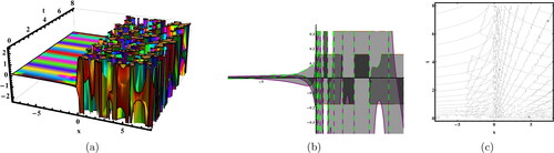
The quadratic–cubic (QC) type is a nonlinear form of refractive index that has recently garnered significant attention. There is a plethora of reported results in both polarization-preserving and birefringent fibers. It is now necessary to shift focus towards the study of soliton dynamics in magneto-optic waveguides. Studying soliton dynamics in magneto-optic waveguides holds significant importance. Magneto-optic elements have the ability to transition solitons from an attractive state to an isolated state. This allows for the management of the phenomenon known as ”soliton clutter”. In the available literature, magneto-optic waveguides with different nonlinear forms has been discussed, such that in Asma et al. (2020) the extended auxiliary equation approach and the unified Riccati equation expansion were the applied and different forms of solutions have been obtained, the traveling wave hypothesis was to used study the optical solitons (Asma et al., 2020). It has been observed that the basic parabolic law of nonlinearity governs the behavior of optical solitons in a waveguide by Zayed et al. (2020). Moreover, the dual-power law nonlinearity was used in waveguides and studied with usage of modified extended direct algebraic method (Ahmed & Rabie, 2021). New mapping method with Kudryashov’s law of refractive index in the waveguides has been discussed (Zayed, Alurrfi, & Alshbear, 2023). However, in this study, we have discussed the fractional affect in the magnet-optic waveguides under QC nonlinear form. The nonlinear Schrödinger’s equation coupled system is regarded as the governing system for the propogation of optical pulses in the magnet-optic waveguides. For observing the parametric behavior on the dynamics of soliton, the graphs have been sketched in the real and imaginary part of the solutions as shown in the Figures (1–9). This article’s findings may be applicable to understanding the structure of many nonlinear progress scenarios that appear in several subfields of nonlinear science.

Figure 1. Sketches of the Eq. (20)(20) $$\begin{array}{l}{p}_1(x,t)=-\frac{3\hspace{0.17em}\mathrm{\text{exp}}\hspace{0.17em}\left(\frac{i\Gamma (\beta +1)\left(\frac{t^{ϵ}\left({\kappa }^2\left(a_1+\zeta {\mathrm{a}}_2\right)+f_2-\zeta {\mathrm{f}}_1+\kappa \left(\zeta {\sigma }_2-{\sigma }_1\right)\right)}{1-\frac{\Gamma (\beta +1)\left(x^{ϵ}-\rho t^{ϵ}\right)}{ϵ}}+\phi -\kappa x^{ϵ}\right)}{ϵ}\right)}{{\Gamma }_2}\\ \times \left({\phi }_1-i\sqrt{2}\sqrt{{\phi }_1}\sqrt{-\frac{{\phi }_1}{{\phi }_2}}\sqrt{{\phi }_2}\text{sech}\left(\sqrt{{\phi }_1}\left(\frac{\Gamma (\beta +1)\left(x^{ϵ}-\rho t^{ϵ}\right)}{ϵ}+\vartheta \right)\right)\right).\end{array}$$(20) for $ϵ=0.6.$

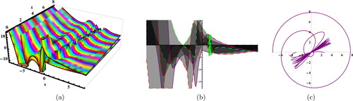
Figure 2. Sketches of the Eq. (22)(22) $$\begin{array}{l}{p}_3(x,t)=\frac{3\hspace{0.17em}\mathrm{\text{exp}}\hspace{0.17em}\left(\frac{i\Gamma (\beta +1)\left(\frac{ϵt^{ϵ}\left(\kappa \left(\kappa \left(a_1+\zeta {\mathrm{a}}_2\right)+\zeta {\sigma }_2-{\sigma }_1\right)+f_2-\zeta {\mathrm{f}}_1\right)}{\Gamma (\beta +1)\left(\rho t^{ϵ}-x^{ϵ}\right)+ϵ}+\phi -\kappa x^{ϵ}\right)}{ϵ}\right)}{{\Gamma }_2}\\ \times \left(-1+\frac{2i\sqrt{2}\sqrt{{\beta }_1{\beta }_2}{e}^{\sqrt{{\phi }_1}\left(\frac{\Gamma (\beta +1)\left(x^{ϵ}-\rho t^{ϵ}\right)}{ϵ}+\vartheta \right)}}{{\beta }_1{e}^{2\sqrt{{\phi }_1}\left(\frac{\Gamma (\beta +1)\left(x^{ϵ}-\rho t^{ϵ}\right)}{ϵ}+\vartheta \right)}-{\beta }_2}\right){\phi }_1.\end{array}$$(22) for $ϵ=0.2.$

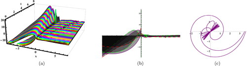
Figure 3. Sketches of the Eq. (25)(25) $$\begin{array}{l}{p}_6(x,t)=-\frac{3\hspace{0.17em}\mathrm{\text{exp}}\hspace{0.17em}\left(\frac{i\Gamma (\beta +1)\left(\frac{ϵt^{ϵ}\left(a_1{\kappa }^2+f_2+\zeta {\mathrm{a}}_2{\kappa }^2-\zeta {\mathrm{f}}_1+\zeta {\sigma }_2\kappa -\kappa {\sigma }_1\right)}{\Gamma (\beta +1)\left(\rho t^{ϵ}-x^{ϵ}\right)+ϵ}+\phi -\kappa x^{ϵ}\right)}{ϵ}\right)}{{\Gamma }_2}\\ \times \sqrt{{\phi }_1}(\sqrt{{\phi }_1}-\sqrt{-\frac{{\phi }_1}{{\phi }_2}}\sqrt{{\phi }_2}(\text{sech}\left(\sqrt{2}\sqrt{-{\phi }_1}\left(\frac{\Gamma (\beta +1)\left(x^{ϵ}-\rho t^{ϵ}\right)}{ϵ}+\vartheta \right)\right)\\ +i\mathrm{\text{tanh}}\left(\sqrt{2}\sqrt{-{\phi }_1}\left(\frac{\Gamma (\beta +1)\left(x^{ϵ}-\rho t^{ϵ}\right)}{ϵ}+\vartheta \right)\right))).\end{array}$$(25) for $ϵ=0.67.$

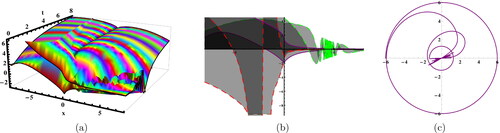
Figure 4. Sketches of the Eq. (29)(29) $$\begin{array}{l}{p}_{10}(x,t)=\frac{\hspace{0.17em}\mathrm{\text{exp}}\hspace{0.17em}\left(\frac{i\Gamma (\beta +1)\left(\frac{ϵt^{ϵ}\left(\kappa \left(\kappa \left(a_1+\zeta {\mathrm{a}}_2\right)+\zeta {\sigma }_2-{\sigma }_1\right)+f_2-\zeta {\mathrm{f}}_1\right)}{\Gamma (\beta +1)\left(\rho t^{ϵ}-x^{ϵ}\right)+ϵ}+\phi -\kappa x^{ϵ}\right)}{ϵ}\right)}{\sqrt{{\Gamma }_1}}\\ \left(\sqrt{2}\sqrt{-\frac{{\phi }_1}{{\phi }_2}}\sqrt{{\phi }_2}\mathrm{\text{csc}}\left(\sqrt{-{\phi }_1}\left(\frac{\Gamma (\beta +1)\left(x^{ϵ}-\rho t^{ϵ}\right)}{ϵ}+\vartheta \right)\right)-i\sqrt{{\phi }_1}\right).\end{array}$$(29) for $ϵ=0.545.$

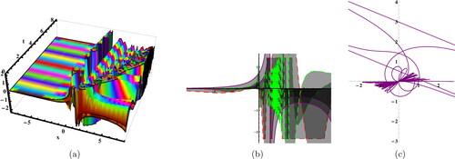
Figure 5. Sketches of the Eq. (33)(33) $$\begin{array}{l}{p}_{14}(x,t)=\frac{\sqrt{{\phi }_1}\hspace{0.17em}\mathrm{\text{exp}}\hspace{0.17em}\left(\frac{i\Gamma (\beta +1)\left(\frac{ϵt^{ϵ}\left(\kappa \left(\kappa \left(a_1+\zeta {\mathrm{a}}_2\right)+\zeta {\sigma }_2-{\sigma }_1\right)+f_2-\zeta {\mathrm{f}}_1\right)}{\Gamma (\beta +1)\left(\rho t^{ϵ}-x^{ϵ}\right)+ϵ}+\phi -\kappa x^{ϵ}\right)}{ϵ}\right)}{\sqrt{{\Gamma }_1}} \\ \times (\frac{4\sqrt{2}\sqrt{{\phi }_1}\sqrt{{\phi }_2}{e}^{\sqrt{{\phi }_1}\left(\frac{\Gamma (\beta +1)\left(x^{ϵ}-\rho t^{ϵ}\right)}{ϵ}+\vartheta \right)}}{4{\phi }_1{\phi }_2{e}^{2\sqrt{{\phi }_1}\left(\frac{\Gamma (\beta +1)\left(x^{ϵ}-\rho t^{ϵ}\right)}{ϵ}+\vartheta \right)}-1}-i).\end{array}$$(33) for $ϵ=0.45.$

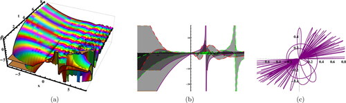
Figure 6. Sketches of the Eq. (37)(37) $$\begin{array}{l}{p}_2(x,t)=\frac{6\hspace{0.17em}\mathrm{\text{exp}}\hspace{0.17em}\left(\frac{i\Gamma (\beta +1)\left(\frac{ϵt^{ϵ}\left(\frac{{\left({\sigma }_1-{\sigma }_2\right)}^2\left(a_1+\zeta {\mathrm{a}}_2\right)}{4{\left(a_1-a_2\right)}^2}+\frac{\left({\sigma }_2-{\sigma }_1\right)\left(\zeta {\sigma }_2-{\sigma }_1\right)}{2\left(a_1-a_2\right)}+f_2-\zeta {\mathrm{f}}_1\right)}{\Gamma (\beta +1)\left(\rho t^{ϵ}-x^{ϵ}\right)+ϵ}+\frac{\left({\sigma }_1-{\sigma }_2\right)x^{ϵ}}{2\left(a_1-a_2\right)}+\phi \right)}{ϵ}\right)}{{\Gamma }_2}\\ \times \left(\sqrt{-{\delta }_0}-i\sqrt{{\delta }_0}\mathrm{\text{ tanh}}\left(\frac{\sqrt{-{\delta }_0}\Gamma (\beta +1)\left(x^{ϵ}-\rho t^{ϵ}\right)}{ϵ}\right)\sqrt{-{\delta }_0}\right).\end{array}$$(37) for $ϵ=0.29.$

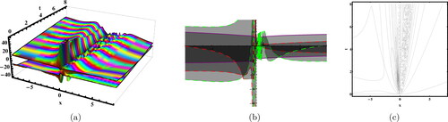
Figure 7. Sketches of the Eq. (40)(40) $$\begin{array}{l}{p}_5(x,t)=\frac{6\hspace{0.17em}\mathrm{\text{exp}}\hspace{0.17em}\left(\frac{i\Gamma (\beta +1)\left(\frac{ϵt^{ϵ}\left(\frac{{\left({\sigma }_1-{\sigma }_2\right)}^2\left(a_1+\zeta {\mathrm{a}}_2\right)}{4{\left(a_1-a_2\right)}^2}+\frac{\left({\sigma }_2-{\sigma }_1\right)\left(\zeta {\sigma }_2-{\sigma }_1\right)}{2\left(a_1-a_2\right)}+f_2-\zeta {\mathrm{f}}_1\right)}{\Gamma (\beta +1)\left(\rho t^{ϵ}-x^{ϵ}\right)+ϵ}+\frac{\left({\sigma }_1-{\sigma }_2\right)x^{ϵ}}{2\left(a_1-a_2\right)}+\phi \right)}{ϵ}\right)}{{\Gamma }_2}\\ \times \left(-1+\frac{i\sqrt{{\delta }_0}\left(4\mathrm{\text{sinh}}\left(\frac{2\sqrt{-{\delta }_0}\Gamma (\beta +1)\left(x^{ϵ}-\rho t^{ϵ}\right)}{ϵ}\right)+3\right)}{\sqrt{-{\delta }_0}\left(4\mathrm{\text{cosh}}\left(\frac{2\sqrt{-{\delta }_0}\Gamma (\beta +1)\left(x^{ϵ}-\rho t^{ϵ}\right)}{ϵ}\right)-5\right)}\right){\delta }_0.\end{array}$$(40) for $ϵ=0.331.$

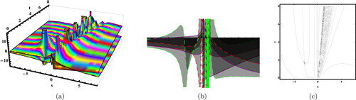
Figure 8. Sketches of the Eq. (41)(41) $$\begin{array}{l}{p}_6(x,t)=\frac{6\hspace{0.17em}\mathrm{\text{exp}}\hspace{0.17em}\left(\frac{i\Gamma (\beta +1)\left(\frac{ϵt^{ϵ}\left(\frac{{\left({\sigma }_1-{\sigma }_2\right)}^2\left(a_1+\zeta {\mathrm{a}}_2\right)}{4{\left(a_1-a_2\right)}^2}+\frac{\left({\sigma }_2-{\sigma }_1\right)\left(\zeta {\sigma }_2-{\sigma }_1\right)}{2\left(a_1-a_2\right)}+f_2-\zeta {\mathrm{f}}_1\right)}{\Gamma (\beta +1)\left(\rho t^{ϵ}-x^{ϵ}\right)+ϵ}+\frac{\left({\sigma }_1-{\sigma }_2\right)x^{ϵ}}{2\left(a_1-a_2\right)}+\phi \right)}{ϵ}\right)}{{\Gamma }_2} \\ \times \left(-1+\frac{i\sqrt{{\delta }_0}\left(c\mathrm{\text{sinh}}\left(\frac{2\sqrt{-{\delta }_0}\Gamma (\beta +1)\left(x^{ϵ}-\rho t^{ϵ}\right)}{ϵ}\right)+d\right)}{4c\sqrt{-{\delta }_0}\mathrm{\text{cosh}}\left(\frac{2\sqrt{-{\delta }_0}\Gamma (\beta +1)\left(x^{ϵ}-\rho t^{ϵ}\right)}{ϵ}\right)-\lambda \sqrt{{\delta }_0\left(-\left(c^2+d^2\right)\right)}}\right){\delta }_0.\end{array}$$(41) for $ϵ=.41.$

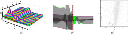
Figure 9. Sketches of the Eq. (44)(44) $$\begin{array}{l}{p}_9(x,t)=\frac{1}{2}\mathrm{\text{exp}}\hspace{0.17em}\left(\frac{i\Gamma (\beta +1)\left(\frac{\left({\sigma }_1-{\sigma }_2\right)x^{ϵ}}{2\left(a_1-a_2\right)}+\omega t^{ϵ}+\phi \right)}{ϵ}\right) \\ \times \left(2+\frac{\sqrt{2}\left(\left(1-{\delta }_0\right)\hspace{0.17em}\mathrm{\text{tan}}\hspace{0.17em}\left(\frac{2\sqrt{{\delta }_0}\Gamma (\beta +1)\left(x^{ϵ}-\rho t^{ϵ}\right)}{ϵ}\right)+\left({\delta }_0+1\right)\hspace{0.17em}\text{sec}\hspace{0.17em}\left(\frac{2\sqrt{{\delta }_0}\Gamma (\beta +1)\left(x^{ϵ}-\rho t^{ϵ}\right)}{ϵ}\right)\right)}{\sqrt{{\delta }_0}}\right){\varphi }_0.\end{array}$$(44) for $ϵ=.22.$

6. Conclusions

In this article, the M-truncated coupled NLSE with the QC form has been taken as the studied model in the mageto-optic waveguides. The different shapes of the solution like, bright, dark, singular and combo solitons, as well as hyperbolic, exponential and periodic solutions successfully extracted with the use of improved sardar subequation method and enhanced modified extended tanh-expansion method. In the electromagnetic field, it is essential to incorporate magneto-optic effect in optical waveguides. As a result, solitons go from being attracted to one another to being isolated. Thus, it is feasible to diminish the amount of information that flows from pulse to pulse. The optical solitons play vital role as information carrier in telecommunication systems, optical industry. In modern days, websites, internet industry, twitter, face book and google are working with the help of optical solitons. The applied approach is highly effective mathematical techniques that are employed to interpret non-linear models in the fields of physics and applied mathematics. The utilization of soliton solutions and the exploration of their inherent physical characteristics contribute significantly to the advancement of non-linear dynamics. The method offers vital insights into complicated processes and facilitate their application in various fields, including communication engineering and physics. The physical movements of the observed solutions are demonstrated by generating 3D, 2D, contour and polar plots by assigning the different values of the parameters. It is our hope that the methodology and outcomes will contribute to the comprehension of physical behavior dynamics and aid researchers to understand the nonlinear issues.

Competing interest

No conflict of interest.

Acknowledgement

This work was supported by the Ministry of Education, Youth and Sports of the Czech Republic through the e-INFRA CZ (ID:90254).

Data availability statement

Not applicable.

Disclosure statement

No potential conflict of interest was reported by the author(s).

References

- Ahmed, H. M., & Rabie, W. B. (2021). Structure of optical solitons in magneto-optic waveguides with dual-power law nonlinearity using modified extended direct algebraic method. Optical & Quantum Electronics, 53(8), 438. doi:10.1007/s11082-021-03026-3
- Akinyemi, L., Şenol, M., Tasbozan, O., & Kurt, A. (2022). Multiple-solitons for generalized-dimensional conformable Korteweg-de Vries-Kadomtsev–Petviashvili equation. Journal of Ocean Engineering & Science, 7(6), 536–542. doi:10.1016/j.joes.2021.10.008
- Akinyemi, L. P., Veeresha, M. T., Darvishi, H. R., Şenol, M., & Akpan, U. (2024). A novel approach to study generalized coupled cubic Schrödinger–Korteweg-de Vries equations. Journal of Ocean Engineering & Science, 9, 13–24.
- Akram, S., Ahmad, J., Rehman, S. U., & Ali, A. (2023). New family of solitary wave solutions to new generalized Bogoyavlensky–Konopelchenko equation in fluid mechanics. International Journal of Applied & Computational Mathematics, 9(5), 63. doi:10.1007/s40819-023-01542-2
- Alshammari, S., Al-Sawalha, M. M., & Shah, R. (2023). Approximate analytical methods for a fractional-order nonlinear system of Jaulent–Miodek equation with energy-dependent Schrödinger potential. Fractal & Fractional, 7(2), 140. doi:10.3390/fractalfract7020140
- Alshehry, A. S., Yasmin, H., Ghani, F., Shah, R., & Nonlaopon, K. (2023). Comparative analysis of advection–dispersion equations with Atangana–Baleanu fractional derivative. Symmetry, 15(4), 819. doi:10.3390/sym15040819
- Altawallbeh, Z., Az-Zo’bi, E., Alleddawi, A. O., Şenol, M., & Akinyemi, L. (2022). Novel liquid crystals model and its nematicons. Optical & Quantum Electronics, 54(12), 861. doi:10.1007/s11082-022-04279-2
- Asma, M., Biswas, A., Kara, A. H., Zayed, E. M. E., Guggilla, P., Khan, S., … Belic, M. R. (2020). A pen-picture of solitons and conservation laws in magneto-optic waveguides having quadratic–cubic law of nonlinear refractive index. Optik, 223, 165330. doi:10.1016/j.ijleo.2020.165330
- Esen, H., Ozisik, M., Secer, A., & Bayram, M. (2022). Optical soliton perturbation with Fokas–Lenells equation via enhanced modified extended tanh-expansion approach. Optik, 267, 169615. doi:10.1016/j.ijleo.2022.169615
- Han, T., Li, Z., & Li, C. (2023). Bifurcation analysis, stationary optical solitons and exact solutions for generalized nonlinear Schrödinger equation with nonlinear chromatic dispersion and quintuple power-law of refractive index in optical fibers. Physica A: Statistical Mechanics & its Applications, 615, 128599. doi:10.1016/j.physa.2023.128599
- Han, T., Tang, C., Zhang, K., & Zhao, L. (2023). Chaotic behavior and traveling wave solutions of the fractional stochastic Zakharov system with multiplicative noise in the Stratonovich sense. Results in Physics, 48, 106404. doi:10.1016/j.rinp.2023.106404
- Ibrahim, S., Sulaiman, T. A., Yusuf, A., Ozsahin, D. U., & Baleanu, D. (2024). Wave propagation to the doubly dispersive equation and the improved Boussinesq equation. Optical & Quantum Electronics, 56(1), 20. doi:10.1007/s11082-023-05571-5
- Jamal, A., Ullah, A., Ahmad, S., Sarwar, S., & Shokri, A. (2023). A survey of (2 + 1)-dimensional KdV–mKdV equation using nonlocal Caputo fractal–fractional operator. Results in Physics, 46, 106294. doi:10.1016/j.rinp.2023.106294
- Mathanaranjan, T. (2023). New Jacobi elliptic solutions and other solutions in optical metamaterials having higher-order dispersion and its stability analysis. International Journal of Applied & Computational Mathematics, 9(5), 66. doi:10.1007/s40819-023-01547-x
- Mathanaranjan, T. (2023). Optical soliton, linear stability analysis and conservation laws via multipliers to the integrable Kuralay equation. Optik, 290, 171266. doi:10.1016/j.ijleo.2023.171266
- Mathanaranjan, T. (2023). Optical solitons and stability analysis for the new (3 + 1)-dimensional nonlinear Schrödinger equation. Journal of Nonlinear Optical Physics & Materials, 32(02), 2350016. doi:10.1142/S0218863523500169
- Mathanaranjan, T., & Vijayakumar, D. (2022). New soliton solutions in nano-fibers with space–time fractional derivatives. Fractals, 30(07), 2250141. doi:10.1142/S0218348X22501419
- Mathanaranjan, T., Kumar, D., Rezazadeh, H., & Akinyemi, L. (2022). Optical solitons in metamaterials with third and fourth order dispersions. Optical & Quantum Electronics, 54(5), 271. doi:10.1007/s11082-022-03656-1
- Mirzazadeh, M., Sharif, A., Hashemi, M. S., Akgül, A., & El Din, S. M. (2023). Optical solitons with an extended (3 + 1)-dimensional nonlinear conformable Schrödinger equation including cubic–quintic nonlinearity. Results in Physics, 49, 106521. doi:10.1016/j.rinp.2023.106521
- Nasreen, N., Lu, D., Zhang, Z., Akgül, A., Younas, U., Nasreen, S., & Al-Ahmadi, A. N. (2023). Propagation of optical pulses in fiber optics modelled by coupled space–time fractional dynamical system. Alexandria Engineering Journal, 73, 173–187. doi:10.1016/j.aej.2023.04.046
- Raza, N., Rani, B., Chahlaoui, Y., & Shah, N. A. (2023). A variety of new rogue wave patterns for three coupled nonlinear Maccari’s models in complex form. Nonlinear Dynamics, 111(19), 18419–18437. doi:10.1007/s11071-023-08839-3
- Raza, N., Salman, F., Butt, A. R., & Gandarias, M. L. (2023). Lie symmetry analysis, soliton solutions and qualitative analysis concerning to the generalized q-deformed Sinh–Gordon equation. Communications in Nonlinear Science & Numerical Simulation, 116, 106824. doi:10.1016/j.cnsns.2022.106824
- Shah, N. A., Agarwa, P., Chung, J. D., El-Zahar, E. R., & Hamed, Y. S. (2020). Analysis of optical solitons for nonlinear Schrödinger equation with detuning term by iterative transform method. Symmetry, 12(11), 1850. doi:10.3390/sym12111850
- Sousa, J. C., & Oliveira, E. C. D. (2018). A new truncated M-fractional derivative type unifying some fractional derivative types with classical properties. International Journal of Analysis & Applications, 16, 83–96.
- Tripathy, A., Sahoo, S., Rezazadeh, H., Izgi, Z. P., & Osman, M. S. (2023). Dynamics of damped and undamped wave natures in ferromagnetic materials. Optik, 281, 170817. doi:10.1016/j.ijleo.2023.170817
- Younas, U., Ren, J., Sulaiman, T. A., Bilal, M., & Yusuf, A. (2022). On the lump solutions, breather waves, two-wave solutions of (2 + 1)-dimensional Pavlov equation and stability analysis. Modern Physics Letters B, 36(14), 2250084. doi:10.1142/S0217984922500841
- Younas, U., Sulaiman, T. A., & Ren, J. (2022). On the collision phenomena to the (3 + 1)-dimensional generalized nonlinear evolution equation: Applications in the shallow water waves. The European Physical Journal Plus, 137(10), 1166. doi:10.1140/epjp/s13360-022-03401-3
- Younas, U., Yao, F., Ismael, H. F., Sulaiman, T. A., & Murad, M.A. S. (2024). Sensitivity analysis and propagation of optical solitons in dual-core fiber optics. Optical & Quantum Electronics, 56(4), 548. doi:10.1007/s11082-023-06220-7
- Zayed, E. M. E., & Ibrahim, S. H. (2012). Exact solutions of nonlinear evolution equations in mathematical physics using the modified simple equation method. Chinese Physics Letters, 29(6), 060201. doi:10.1088/0256-307X/29/6/060201
- Zayed, E. M. E., Alngar, M. E. M., Horbaty, M. M. E., Biswas, A., Guggilla, P., Ekici, M., … Belic, M. (2020). Solitons in magneto-optic waveguides with parabolic law nonlinearty. Optik, 222, 165314. doi:10.1016/j.ijleo.2020.165314
- Zayed, E. M. E., Alurrfi, K. A. E., & Alshbear, R. A. (2023). On application of the new mapping method to magneto-optic waveguides having Kudryashov’s law of refractive index. Optik, 287, 171072. doi:10.1016/j.ijleo.2023.171072
- Zhao, Y.-H., Mathanaranjan, T., Rezazadeh, H., Akinyemi, L., & Inc, M. (2022). New solitary wave solutions and stability analysis for the generalized (3 + 1)-dimensional nonlinear wave equation in liquid with gas bubbles. Results in Physics, 43, 106083. doi:10.1016/j.rinp.2022.106083
- Zhu, S. D. (2008). The generalizing Riccati equation mapping method in non-linear evolution equation: Application to (2 + 1)-dimensional Boiti–Leon–Pempinelle equation. Chaos Solit Fractals, 37(5), 1335–1342. doi:10.1016/j.chaos.2006.10.015