Finding the Optimal Number of Persons (N) and Time Points (T) for Maximal Power in Dynamic Longitudinal Models Given a Fixed Budget

Abstract

Planning longitudinal studies can be challenging as various design decisions need to be made. Often, researchers are in search for the optimal design that maximizes statistical power to test certain parameters of the employed model. We provide a user-friendly Shiny app OptDynMo available at https://shiny.psychologie.hu-berlin.de/optdynmo that helps to find the optimal number of persons (N) and the optimal number of time points (T) for which the power of the likelihood ratio test (LRT) for a model parameter is maximal given a fixed budget for conducting the study. The total cost of the study is computed from two components: the cost to include one person in the study and the cost for measuring one person at one time point. Currently supported models are the cross-lagged panel model (CLPM), factor CLPM, random intercepts cross-lagged panel model (RI-CLPM), stable trait autoregressive trait and state model (STARTS), latent curve model with structured residuals (LCM-SR), autoregressive latent trajectory model (ALT), and the latent change score model (LCS).

Keywords:

• Dynamic modeling
• longitudinal modeling
• optimal design
• optimization
• statistical power

Longitudinal modeling has been a core technique in psychological and social science research for a long time. More recently, dynamic longitudinal models (e.g., Voelkle et al., 2018) became increasingly prominent. We refer to longitudinal models as dynamic when they include autoregressive effects (in the univariate case) or autoregressive and cross-lagged effects (in the multivariate case). Popular dynamic longitudinal models are, for instance, the cross-lagged panel model (CLPM; e.g., Selig & Little, 2012), which has been labeled the “workhorse in developmental psychology for decades” (Berry & Willoughby, 2017), and the random intercepts cross-lagged panel model (RI-CLPM; Hamaker et al., 2015) whose popularity is mirrored by over 1700 citations (in Google Scholar, 17 November 2022). Recently, a unified framework that incorporates these and other dynamic longitudinal models has been proposed by Usami et al. (2019).

Researchers who plan to apply dynamic longitudinal models are confronted with various design decisions—one of the most obvious being how many persons should be sampled and how often these persons should be assessed. Such a decision usually needs to be made with respect to some criterion (or criteria). Oftentimes, the statistical power to detect an effect (i.e., to test a model parameter against zero or some other value) is of core interest, for instance, because funding agencies require power calculations for grant proposals and because underpowered studies can lead to biased conclusions and are a waste of the scarce resource participants, as argued by Crutzen and Peters (2017).¹ Hence, researchers might be interested in choosing the number of persons (N) and the number of time points (T) in such a way that the statistical power for model parameters of interest (target parameters) is maximal under the constraint of a fixed budget.

How could researchers achieve to identify this optimal N–T–combination for maximal power? One standard approach for power calculation is Monte Carlo simulation (e.g., Muthén & Muthén, 2002). Here, the researcher needs to run the model on thousands of generated data sets and record how often the false null hypothesis is rejected. This yields power estimates for model parameters for one specific combination of N and T values. Finding the optimal N–T–combination then requires researchers to consider large and fine-grained ranges of possible N and T values, making this simulative search computationally very intensive. Also, setting up simulations requires some level of programming skills.

Instead of conducting the simulations oneself, researchers could rely on published results from studies that investigated how different design parameters affect power. In fact, many such studies exist, for example, by Fan (2003), Hertzog et al. (2006, 2008), von Oertzen et al. (2010), and Wu et al. (2016), to name just a few. However, researchers then must be lucky that results and recommendations for exactly their desired model and model parameter(s) are available. For growth models, quite some insights are available that can help with designing longitudinal studies (e.g., Brandmaier et al. (2015, 2020); Muthén & Curran, 1997; Fan, 2003; Hertzog et al., 2006, Hertzog et al., 2008; von Oertzen, 2010; von Oertzen et al., 2010; von Oertzen & Brandmaier, 2013; Wu et al., 2016). Yet, for dynamic models, advice seems to be much sparser.

Purpose and Scope

In this work, we propose an approach and algorithm to calculate the optimal N and T to maximize statistical power for parameters from a popular set of dynamic models. We programmed the Shiny app OptDynMo with which researchers can optimize their longitudinal study designs easily and fast.

In a nutshell, our approach is based on Satorra and Saris’ (1985) closed-form power calculations for the likelihood ratio test (LRT) and a numerical optimization procedure which searches for the N and T that maximize power for the desired target parameters given a fixed budget. The numerical optimization is performed with the R package rgenoud (Mebane & Sekhon, 2011).

The article is organized into the following sections. First, we summarize previous work on power calculation and design optimization. Second, we describe our approach and give technical details on its implementation. Third, we give a tutorial-like introduction on how to use our Shiny app which is the central product of our presented work. Fourth, we discuss limitations of our app and sketch potential future extensions.

Previous Research

Searching for optimal designs has a decades-long tradition in the social sciences with an extensive body of literature. The ingredients for optimal design research often are (1) criteria that are the target of optimization and methods to compute these criteria, (2) the design parameters and constraints, and (3) algorithms and methods to conduct the search within the design parameter space.

Optimization Criteria

Statistical power is often deemed one of the important metrics for the quality of a study, because it provides the probability of a significant result (e.g., von Oertzen, 2010; von Oertzen & Brandmaier, 2013), or as Jak et al. (2021) put it: “When statistical power is too low to detect a meaningful effect, a study would essentially waste data on type II errors.” (p. 1385). Power thus has been a desired target for optimization (or more precisely, maximization); for example, Allison et al. (1997) address the question: “Given a fixed amount of money, what is the maximum power that I can achieve?” (p. 20).

If power is the target of optimization, obviously a method to compute the power is needed. This task could be done via Monte Carlo simulations (e.g., Muthén & Muthén, 2002; Wang & Rhemtulla, 2021) or with calculation formulas. Whereas Monte Carlo simulations are very flexible, they might become computationally very demanding and thus very time-consuming. Therefore, their applicability for design optimizations, where power needs to be calculated many times, is limited. Formulas for power calculations are usually computationally much less demanding, but often have a limited scope and/or precision. For example, for a special dynamic longitudinal model, the continuous-time VAR(1) model, Hecht and Zitzmann (2021) proposed such a formula to approximate power for peak cross-lagged effects which they derived from heavy simulations in combination with machine-learning techniques. However, it is oftentimes better to employ analytically derived formulas. For a variety of simple tests and models, such power formulas are available and packed into user-friendly tools such as G*Power (Faul et al., 2007) or the R package pwr (Champely, 2020). For multi-level models with AR(1) within-person errors, Lafit et al. (2023) derived analytical formulas for statistical power. For structural equation models (SEMs), Satorra and Saris (1985) proposed an approach for power calculations for the LRT and MacCallum, Browne, and Sugawara (1996) for power calculations based on the root mean square error of approximation (RMSEA). Both methods were implemented into the user-friendly Shiny app power4SEM by Jak et al. (2021). Another software application for power calculations is Jrule (Oberski, 2009), which reads in Mplus output with modification indices and expected parameter change information and provides a user interface to taking into account the power of the score test as described by Saris, Satorra, and van der Veld (2009). Research and tools aimed at power calculations for longitudinal modeling for example consist of the R package and Shiny app longpower developed by Iddi and Donohue (2022), the Shiny apps PowerAnalysisIL and PowerLAPIM created by Lafit et al. (2021, 2022), the works of Liu and Liang (1997), Lu et al. (2008), Moerbeek (2022), Basagaña and Spiegelman (2010), Basagaña et al. (2011), and Bolger et al. (2012).

Design Parameters and Constraints for the Optimization

After the target of optimization has been defined (e.g., power), the design parameters that can vary and their admissible range need to be determined. Together with optional further design constraints (e.g., imposed by a cost function), this defines the search space for the optimization. Many authors have proposed cost functions (e.g., Allison, 1995; Allison, 1997; Tekle et al., 2011; van Breukelen, 2013; Zitzmann et al., 2022). For a two-level context, van Breukelen (2013) and Zitzmann et al. (2022) suggested to calculate the total study cost as a function of the numbers of level-2 and level-1 units and the costs that are associated with including and assessing these level-2 and level-1 units in the study. With such a cost function, Zitzmann et al. (2022) reduced the search space from two to one dimension, because the sample size of one level can be expressed as a function of the sample size of the other level.

Besides sample size, many other design parameters could be used for the optimization. For example, Adolf et al. (2021) searched for the optimal sampling rates for continuous-time first-order autoregressive and vector autoregressive models,² Wu et al. (2016) and Brandmaier et al. (2020) searched for optimal planned missingness patterns for growth-curve modeling, Tekle et al. (2011) included the number of cohorts (besides number of measurement occasions) in their optimization of designs for linear mixed-effect models, Schlesselman (1973) optimized the frequency of measurement and study duration, and Raudenbush and Liu (2001) showed that power depends on a standardized effect size, the sample size, and a person-specific reliability coefficient which in turn depends on study duration and frequency of observation.

Optimization Methods

After the design parameters for the optimization have been defined, some method is needed to conduct the search for optimal values of these design parameters. One frequently employed option is to use numerical optimization routines and algorithms. For example, Adolf et al. (2021) and Zitzmann et al. (2022) both used R’s general-purpose optimizer optim() (R Core Team, 2022). Instead of numerical optimization, von Oertzen (2010) approached the optimization task of cost reduction given a fixed target power by employing power-equivalent model modification operations, an approach that has been picked up in a series of articles (von Oertzen & Brandmaier, 2013; Brandmaier et al., 2015; Brandmaier et al., 2020) and incorporated into the tool Longitudinal Interactive Front End Study Planner (LIFESPAN; Brandmaier et al., 2015).

To summarize, researchers who plan a longitudinal study and want to optimize the design, need to think about the target criteria, the design parameters and constraints for the optimization, and the method of optimization. In previous research, target criteria were often study cost or power (primarily for the class of growth models), the design parameters often were the number of persons (N), the number of time points (T), study duration, or planned missingness patterns, and methods for optimization were numerical optimization algorithms or special model modification rules.

In principal, researchers might not have to bother with implementing and programming the design optimization and power calculation routines³ themselves if tools are available, and they are (e.g., the excellent tools and software packages LIFESPAN, Brandmaier et al., 2015; G*Power, Faul et al., 2007; power4SEM, Jak et al., 2021; OD, Raudenbush et al., 2011; Ml-des, Cools et al., 2008; Jrule, Oberski, 2009; and the Shiny apps by Zitzmann et al., 2022, Hecht & Zitzmann, 2021, Lafit et al., 2021, 2022, and Iddi & Donohue, 2022). However, for finding the optimal N and T that maximize the power for testing parameters from dynamic models, no such tool is—to the best of our knowledge—available.

Procedure for Finding the Optimal N and T for Maximal Power

The goal of our optimization procedure is to find the number of persons (N) and the number of time points (T) for which the statistical power of tests for one or more model parameters is maximal given a fixed budget. In a nutshell, our procedure uses the genoud optimizer to search over T for maximal power with N being determined via the cost function. Technical details are given in the next subsections. Our optimization procedure is the core of our user-friendly Shiny app OptDynMo, which is described further below.

Cost Function

In line with van Breukelen (2013; see also Zitzmann et al., 2022), we assume that the total cost for a study (and thus the budget B that is needed) is the sum of the cost for one person (C₂) times the number of persons (N) and the cost for one measurement (C₁) times the number of time points (T) times the number of persons: (1) $$B=C_{2}N+C_{1}TN.$$(1)

The required number of persons N can therefore be calculated as: (2) $$N=\frac{B}{C_2+C_{1}T}.$$(2)

As N is a function of T, it is sufficient to use T as the parameter over which the optimization is performed.

Objective Function

The objective function gets T as input and then computes N via Eq. 2(2) $$N=\frac{B}{C_2+C_{1}T}.$$(2) . After that, the power for each model parameter is calculated. These power calculations are conducted with Satorra and Saris’ (1985) SEM-LRT approach for a significance level $\alpha$ and the null hypothesis that the parameter is zero in the population. We chose Satorra and Saris’ approach primarily because it is a computationally very efficient approximation, allowing for rapid optimizations. Moreover, Satorra and Saris report high accuracy, especially when the value of the tested parameter is close to the value under the null hypothesis (which is zero in our approach). When optimizing power for multiple target parameters, our procedure assumes a separate LRT for each target parameter at the specified significance level α. If users wish to correct for multiple testing, they will need to do so themselves.

Power Calculation

In the following, we briefly summarize the method to approximate the power of the LRT put forward by Satorra and Saris (1985). Let (3) $$F(\mathbf{S},\mathbf{\Sigma }(\mathbf{\theta }))=\mathrm{tr}\left(\mathbf{S}\hspace{0.17em}\mathbf{\Sigma }{(\mathbf{\theta })}^{-1}\right)-\hspace{0.17em}\ln \hspace{0.17em}\left(\left|\mathbf{S}\hspace{0.17em}\mathbf{\Sigma }{(\mathbf{\theta })}^{-1}\right|\right)-p$$(3) be the maximum likelihood fitting function used to fit SEMs on multivariate normally distributed data (e.g., Bollen, 1989), where p denotes the number of observed variables, S is the sample covariance matrix of the observed variables, $\mathbf{\Sigma }(\mathbf{\theta })$ is the corresponding model-implied covariance matrix, and $\mathbf{\theta }$ is a vector with q model parameters. Minimizing F yields the maximum likelihood estimates $\widehat{\mathbf{\theta }}$ of the parameters $\mathbf{\theta }.$

By multiplying the fitting function by the sample size and evaluating it at the parameter estimates, we obtain the test statistic TS. When the data are normally distributed and the model is correctly specified, large sample theory (e.g., Ferguson, 1996; Rao, 1973) tells us that TS converges to a central ${\chi }^2$-distribution with $df=p(p+1)/2-q$ degrees of freedom. More formally, we write: (4) $$N·F(\mathbf{S},\mathbf{\Sigma }(\widehat{\mathbf{\theta }}))=\mathit{TS}\stackrel{d}{\to }{\chi }_{df}^2.$$(4)

Now, we consider the hypotheses H₀ and H₁ that imply two different models with corresponding parameter vectors ${\mathbf{\theta }}_{H_0}$ and ${\mathbf{\theta }}_{H_1}.$ In our Shiny app, the model under H₁ is defined by the user who specifies values for ${\mathbf{\theta }}_{H_1}.$ The model under H₀ is obtained by setting one parameter in ${\mathbf{\theta }}_{H_1}$ to zero, yielding ${\mathbf{\theta }}_{H_0}.$ Of course, the parameter set to zero is the one for which we want to determine the power. The LRT is one of the most commonly used procedures to compare the two models. It rejects the null hypothesis when the test statistic (5) $$\mathit{LRT}=N·\left[F(\mathbf{S},\mathbf{\Sigma }({\widehat{\mathbf{\theta }}}_{H_0}))-F(\mathbf{S},\mathbf{\Sigma }({\widehat{\mathbf{\theta }}}_{H_1}))\right]$$(5) exceeds a certain critical value $c_{\alpha }.$ Under the H₀, the test statistic LRT follows asymptotically a central ${\chi }^2$-distribution with r degrees of freedom, where r denotes the difference in degrees of freedom between the models under H₁ and H₀. Note that r is always 1 in our implementation because only a single parameter is tested at a time.

Satorra and Saris (1985) suggest the following analytical procedure to approximate the power of the LRT. They note that in situations, where the model under the H₀ is fitted on data sampled when H₁ is true, the test statistic does not follow the standard ${\chi }^2$-distribution anymore. Instead, the test statistic (6) $$\widetilde{\mathit{TS}}=N·F({\mathbf{S}}_{H_1},\mathbf{\Sigma }({\widehat{\mathbf{\theta }}}_{H_0}))$$(6) lies more to the right, is more spread out, and follows asymptotically a non-central ${\chi }^2$-distribution with df degrees of freedom and non-centrality parameter λ. Satorra and Saris (1985) note that we can approximate the power of the LRT by computing how much of the asymptotic distribution of $\widetilde{\mathit{TS}}$ (that is, the non-central ${\chi }^2$-distribution) lies on the right side of a critical value $c_{\alpha }$ obtained from the asymptotic distribution of TS (the central ${\chi }^2$-distribution). Thus, the asymptotic power of this test is (7) $$P(\widetilde{\mathit{TS}}>c_{\alpha }|H_1)=1-P(\widetilde{\mathit{TS}}\le c_{\alpha }|H_1)=1-F_{{\chi }_{1,\lambda }^2}(c_{\alpha }),$$(7) where $F_{{\chi }_{1,\lambda }^2}$ is the cumulative probability function of the ${\chi }^2$-distribution with df = 1 degree of freedom and non-centrality parameter λ.

All that remains to be done is to compute the quantities $c_{\alpha }$ and λ. The critical value $c_{\alpha }$ can be straightforwardly determined by locating the $1-\alpha$ quantile of the central ${\chi }^2$-distribution with 1 degree of freedom. Computing the non-centrality parameter is more challenging. However, Satorra and Saris (1985) propose the following simple approximation of the non-centrality parameter that involves fitting the model under the H₀ (yielding $\mathbf{\Sigma }({\widehat{\mathbf{\theta }}}_{H_0})$) on the population covariance matrix under the H₁ (that is, ${\mathbf{\Sigma }}_{H_1}$): (8) $$\lambda =N·F({\mathbf{\Sigma }}_{H_1},\mathbf{\Sigma }({\widehat{\mathbf{\theta }}}_{H_0})).$$(8)

Although the abovementioned procedure provides high accuracy (see Satorra & Saris, 1985), it requires fitting the model under the H₀. As a result, calculating the optimal N and T becomes computationally intensive, especially if the search space is large and various possible values for N and T need to be considered. To solve this issue and to provide a responsive user experience, we implemented a computationally less intense two-step procedure that uses a faster approximation of the non-centrality parameter λ. Instead of fitting the model under the H₀ on the population covariance matrix under the H₁, we calculate the difference between both population covariance matrices: (9) $$\tilde{\lambda }=N·F({\mathbf{\Sigma }}_{H_1},{\mathbf{\Sigma }}_{H_0}).$$(9)

This approximation involves no model estimation because the population covariance matrices ${\mathbf{\Sigma }}_{H_1}$ and ${\mathbf{\Sigma }}_{H_0}$ can be straightforwardly computed from the user input to our Shiny app. Although the resulting $\tilde{\lambda }$ is larger than λ, both quantities usually lead to the same optimal N and T. After the optimal N and T have been identified, we re-calculate the power using Satorra and Saris’ (1985) method outlined above.

Models

Our procedure is applicable to a wide range of SEMs, in principle for all models for which Satorra and Saris’ (1985) SEM-LRT approach can provide power statistics. In the current work, we focus on dynamic longitudinal models that are included in Usami et al.’s (2019) “unified framework of longitudinal models to examine reciprocal relations,” which are the CLPM (e.g., Selig & Little, 2012), the factor CLPM (Usami et al., 2019; also known as the autoregressive cross-lagged factor model, Usami et al., 2015, and as the crossed-lagged regression of factors, McArdle, 2009), the RI-CLPM (Hamaker et al., 2015), the stable trait autoregressive trait and state model (STARTS; Kenny & Zautra, 2001; also known as the trait-state-error [TSE] model, Kenny & Zautra, 1995), the latent curve model with structured residuals (LCM-SR; Curran et al., 2014), the autoregressive latent trajectory model (ALT; Bollen & Curran, 2004; Curran & Bollen, 2001), and the latent change score model (LCS; Hamagami & McArdle, 2001; McArdle & Hamagami, 2001). These models are depicted in Figures B1–B7 in the Appendix B.

Figure 1. User interface of Shiny app OptDynMo (available at https://shiny.psychologie.hu-berlin.de/optdynmo).

Note that all of these models are discrete-time models that typically presume a single, constant time interval between measurement occasions. This constraint is removed in the more versatile continuous-time models (see, e.g., Voelkle et al., 2018, for the distinction between discrete-time and continuous-time models), which allow for the investigation of the unfolding and dissipation of effects depending on the time interval (e.g., Hecht & Zitzmann, 2021).

A central assumption underlying our implementations of these models is stationarity in the sense that all model parameters (for $T\ge 2$) do not change over time. In particular, these models are covariance stationary and mean stationary because they assume that the process (co)variances and means remain constant across all time points (see, e.g., Hamilton, 1994, Section 3.1; Brockwell & Davis, 2002, Section 1.4; Enders, 2015, Section 3; Lütkepohl, 2005, Section 2.1.3; Shumway & Stoffer, 2015, Section 1.5). Assuming stationarity, the parameters of the first time point must adhere to this assumption, meaning that the (co)variances at the first time point should be constrained to the process (co)variances, and the means at the first time point should be constrained to the process means.

Optimizer

To formulate the dynamic longitudinal models within the SEM framework and thus to be able to use Satorra and Saris’ (1985) SEM-LRT approach for power calculations, an integer-valued number of time points T is needed, because the time points (which are our level-1 units) are represented as variables (see, e.g., Mehta & Neale, 2005, and Curran, 2003, who discuss the modeling of multi-level models within the SEM framework). Hence, an integer optimizer is needed for our optimization task. We chose the genoud optimizer (genetic optimization using derivatives) implemented in the R package rgenoud (Mebane & Sekhon, 2011) as it provides integer optimization functionality in R, has an intuitive usability, and can optimize multiple criteria at once; this set of requirements quite drastically limited the number of possible optimizers to choose from. In Appendix A we describe how we tuned the optimizer for our optimization task.

Code Availability

Our code is open-source and available at https://github.com/martinhecht/optimalCrossLagged.

Shiny App OptDynMo (Version 0.2.0, June 2023)

The graphical user interface of our Shiny app OptDynMo (available at https://shiny.psychologie.hu-berlin.de/optdynmo) is presented in Figure 1. The app consists of three input panels, an output panel, a tech panel, and references, which are all described next. For user convenience, we enriched the app with helpful advice and descriptions available as mouse-over texts triggered when the user moves the mouse over the question mark symbols.

Study Design

In the input field Budget, the available study budget in arbitrary monetary units can be specified. The $\alpha$-Level input field serves for defining the level of significance for the power calculations. Below these two input fields are two frames with input fields specific to persons and time points. The cost for including one person in the study and the cost for one time point (i.e., one measurement of one person) can be specified in the field Costs. The minimal and maximal number of persons and time points can be set in the fields Min and Max. The default minimum number of time points depend on the chosen model (see below). As the range of number of persons and number of time points is interdependent due to the cost function (see subsection “Cost Function” above), our procedure performs adjustments to these ranges. The adjusted ranges used in the optimization are printed in gray on the right-hand side of the input boxes.

Model Characteristics

In the input field Model Class, the user can choose between various models: CLPM (default), factor CLPM, RI-CLPM, STARTS, LCM-SR, ALT, and LCS. These models are represented in Figures B1–B7 in the Appendix B and also in the app (Panel B). Please be aware that the figures in the app are static and do not reflect the selected parameter values. When one of the models is chosen, the app will adjust the minimal number of time points for stationary model identification as provided by Usami et al. (2019, table 1 on p. 639). In the input text field Process Names, the names of the processes can be specified by comma-separating them (default: “proc1, proc2”). The number of provided names determines the number of processes in the model, which is displayed in a gray box.

Model Parameters

In the panel Model Parameters, the anticipated values⁴ need to be specified for all model parameters. The displayed parameter input fields depend on the model class. The autoregressive and cross-lagged parameters and dynamic residual variance/covariance parameters are always displayed, as these parameter types are part of all supported models. Also, the user can choose the target parameters for which the power calculation is desired by using the provided dropdown menus. For multivariate models (number of processes $\ge 2$), the default target parameters are all cross-lagged effects, whereas for univariate models (1 process), the default target parameter is the autoregressive effect. In the mouse-over texts, information and references on parameter interpretation is provided.

Results

Our app is designed for rapid user experience. Manipulating one input field will automatically trigger the calculations, and results are immediately (usually within less than a second) displayed in the Results section. The results consist of the optimal number of persons (N) and the optimal number of time points (T) for which the power of the LRTs of the target parameters is maximal. These power values for all target parameters are displayed as well.

Technical Details

In the technical details panel, the run time of the optimization process (in seconds) and the number of optimizer iterations is given. For future improvements of the app and the optimization procedure, the app saves all in- and output. Users can stop this by unticking the checkbox labeled “Log Results.” The elapsed time (in seconds) for the saving process (log run time), the log identifier (an auto-increased integer), and whether the saving process was successful (log status) is displayed.

The precision⁵ of the optimizer can be adjusted via a slider ranging from 16 (default) to 1,000. In many cases, the default precision should be sufficient to provide stable results. However, for some parameter constellations, the optimization might become tough for the optimizer and potentially untrustworthy results may occur. Then the warning message “Optimizer results might be of low accuracy. Try to increase the precision of the optimizer (see “Technical details” section) until this message vanishes.” is displayed. The user should then adhere to this suggestion and increase the optimizer precision which, disadvantageously, also leads to longer run times. If the maximal precision (1,000) is selected and results are still identified as potentially unstable, the app issues the warning “Optimizer results might be of low accuracy. Use results with caution!”.

References

References which are cited in the mouse-over texts are listed.

How to Cite

There, users can find information on citing the app and this accompanying article.

Discussion

The purpose of this work was to provide a user-friendly tool for finding the optimal number of persons (N) and number of time points (T) given a fixed study budget that maximizes the power of LRTs for model parameters from the dynamic longitudinal models CLPM, factor CLPM, RI-CLPM, STARTS, LCM-SR, ALT, and LCS. Our tool and optimization procedure shares the fate with all other tools and procedures of being limited in certain aspects. In the following, we discuss these limitations which nevertheless can lay the ground for future extensions of our tool and procedure.

The current version of our tool is limited to the specific dynamic models that Usami et al. (2019) incorporated into their unified framework of longitudinal models to examine reciprocal relations. Although we think that highly popular models are covered, our software could include more models in future versions. Basically, all models that can be specified in the SEM framework are potential candidates. Also, it might be possible to provide a general input interface for specifying any kind of SEM. We had actually started our project with this idea in mind, but then decided to first just provide some specific popular models in an attempt of not overburdening the user. Also an interesting extension to the models discussed by Usami et al. (2019) would be to incorporate multi-group functionality, similar to what Mulder and Hamaker (2021) have done for the RI-CLPM.

Another promising extension to our approach is support for longitudinal models with multiple indicators per latent factor. Following Usami et al. (2019), the measurement part of the models comprise of single indicators. In foresight, we have already prepared our code in such a way that it is easily extensible to multiple indicator measurement models. This would open up the possibility of pursuing interesting design questions like “If we added (or subtracted) measurement occasions, in how far could we afford to use a less reliable (or would we need a more reliable) measurement instrument?” (Brandmaier et al., 2015, p. 6).

In our implementation of Usami et al.’s (2019) models, we assumed stationarity and constrained the parameters of the first time point accordingly. Although we think that this is one of the most common and widely used modeling options, in future versions of our app we could lift the stationarity constraints for the parameters of the first time point and allow for their free estimation and thus for the inclusion in power calculations.

Our approach relies on Satorra and Saris’ (1985) method for power calculations of the LRT. Satorra and Saris’ method suits our app well because it provides a computationally efficient and accurate power approximation. Nevertheless, the method is based on asymptotic theory and thus may be less precise in estimating the power in small samples. One alternative would be the use of Monte Carlo simulations, which may perform better in small samples. However, Monte Carlo simulations would drastically increase the run time of our app and would require more computational resources than we can currently provide. Moreover, especially in very small samples, estimation problems and non-convergence may bias the simulated power, which would not be surprising since many longitudinal models, such as the STARTS, are hard to estimate (see Cole, Martin, & Steiger, 2005; Luhmann et al., 2011, Kenny & Zautra, 2001).

Other optimization criteria besides the maximization of power might be interesting for study designers. For instance, designs could be wanted that minimize study costs for a desired power, thus answering questions like “Given that I need a fixed degree of power, what is the design that costs the least amount of money?” (Allison et al., 1997, p. 20). Such an objective was, for example, in the focus of the research by von Oertzen et al., 2010, von Oertzen & Brandmaier, 2013, Brandmaier et al. (2015, 2020), and also Zitzmann et al. (2022).

We searched over number of time points (T) for maximal power while determining the number of persons (N) via a cost function. Other design parameters and cost functions might be interesting and suitable and have been used in other research. We used a simple cost function adopted from van Breukelen (2013) and Zitzmann et al. (2022), which is in principle also similar to Tekle et al.’s (2011) cost function. These authors assume two cost components, one for including one person in the study and one for measuring a person at one time point. In addition, Raudenbush and Liu (2001) suggest to consider duration, frequency, and sample size in cost functions, and caution against potential participant attrition which might be associated with prolonged study duration. Attrition is also a central theme in the work of Brandmaier et al. (2020) on optimal planned missing data designs for linear latent growth curve models. Adding the capability to include planned missingness to our app would be a valuable and useful feature. However, this complex task requires further research and significant effort and is therefore a long-term goal for our team.

It is also interesting to consider the optimal sampling scheme or, in other words, the optimal length of time intervals between measurement occasions and whether and in case how much within- and/or between-person variation in interval lengths is beneficial. As discrete-time models (such as the models employed in the present work) might not be feasible for neat integration of data from flexible longitudinal designs with intra- and inter-individually varying time intervals, another class of models, that is, continuous-time models (e.g., Hecht et al., 2019; Hecht & Voelkle, 2021; Hecht & Zitzmann, 2020, 2021; Lohmann et al., 2022; Ryan et al., 2018; Voelkle et al., 2012), might prove to be beneficial. Research that started exploring optimal designs for continuous-time models is for, example, the work of Adolf et al. (2021) and Voelkle and Oud (2013).

Our app currently outputs one optimized solution based on the inputted design and model parameters. However, it would be valuable to investigate how sensitive the solutions are to slight modifications of the input parameters. To that end, we made a significant effort to minimize run time so that users can experiment with the input parameters and explore the sensitivity of the results. Further, visualizing power for values of N and T slightly around their optimal values in a power landscape would be a nice potential feature for future updates.

One issue that researchers may face when performing power calculations is the uncertainty surrounding population values. While suggestions have been made in the literature, such as those by Taylor and Muller (1995, 1996) and Anderson et al. (2017), on how to account for this uncertainty, our app does not currently implement these methods. In the meantime, users can conduct sensitivity analyses by varying input values. For instance, Harrall et al. (2023) suggest considering values that are double or half the original hypothesized value and examining their effects on power.

Our Shiny app OptDynMo is part of a series of excellent tools and software packages (as mentioned above), such as Jak et al.’s (2021) Shiny app power4SEM, which is also based on Satorra and Saris’ (1985) closed-form power calculations and is highly adaptable to different models. OptDynMo goes beyond calculating power for a user-specified model by searching for optimal design parameters (N and T) to maximize power under a fixed budget. Although our approach is generally applicable to all SEMs that can be handled by power4SEM, we decided to provide an easy-to-use interface for optimizing designs for popular longitudinal models. Extending our app to include power4SEM’s highly adaptable SEM input in lavaan syntax would be an intriguing option.

Optimizing longitudinal study designs is a complex endeavor, but worth the effort. We hope that researchers find our tool helpful for planning their longitudinal studies.

Notes

1 But see Zitzmann et al. (2023) who argue that “underpowered” studies might still be useful for meta-analytical research.

2 Note that Adolf et al. (2021) derived a closed-form expression of the optimal sampling rate for a continuous-time AR(1) process, whereas numerical optimization was used for bivariate VAR(1) processes.

3 Note that closed-form solutions may be available or derived for both tasks of determining power and searching for an optimal design, or alternatively, simulative/numerical procedures can be employed.

4 Assumed population values for the input parameters might, for instance, be obtained from previous studies or experts in the specific research area (also see, for instance, Harrall et al., 2023, for recommendations on how to extract relevant inputs from literature and how to conduct and report power analyses). As our app has a short run time, users can easily explore the sensitivity of the results by inputting various assumed population values if there is uncertainty about them.

5 We use the term “precision” as a user-friendly transcription of what the argument pop.size of the genoud optimizer adjusts, see Mebane and Sekhon (2011) and Appendix A.

Appendix A.

Tuning the Optimizer

The genoud optimizer uses an evolutionary algorithm with the most important tuning option being the so-called population size (see Mebane & Sekhon, 2011, for explanations of how the optimizer works and what parameters can be modified). Increasing the population size increases the reliability of the solution, but also lengthens computational time—hence, trade-offs must be made. Unfortunately, as the authors of the optimizer note, “…because of the stochastic nature of the algorithm, it is impossible to generally answer the question of what is the best population size to use” (Mebane & Sekhon, 2011, p. 7). Therefore, we conducted a small simulation where we varied the population size (2, 4, 6, 10, 16, 20, 26, 30, 36, 40, 46, 50, 100). For each population size we conducted 1,000 optimization runs for a bivariate CLPM (the true parameter values are provided in the code of function generate.model.example.2() in our code repository on GitHub, https://github.com/martinhecht/optimalCrossLagged); default values for the other options of the optimizer (rgenoud version 5.9-0.3) were used, except for wait.generations and boundary.enforcement which were set to 1 and 2, respectively). The goal was to identify the smallest population size for which the solution is stable, that is, when the solution (i.e., the optimal T) does not vary over optimization runs. This was the case for all investigated population sizes $\ge 16.$

Appendix B.

Model Diagrams

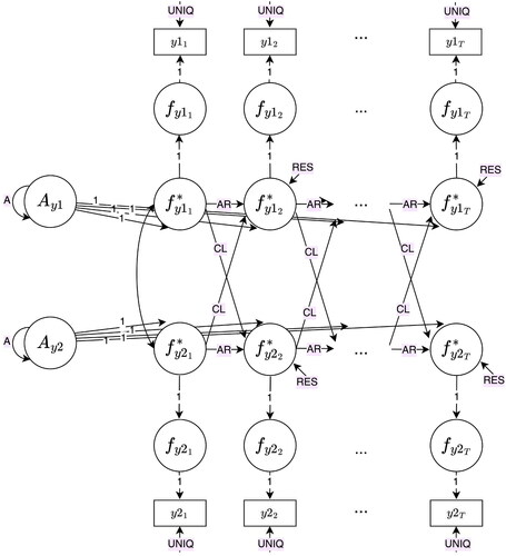
Figure B1. Cross-lagged panel model (CLPM).

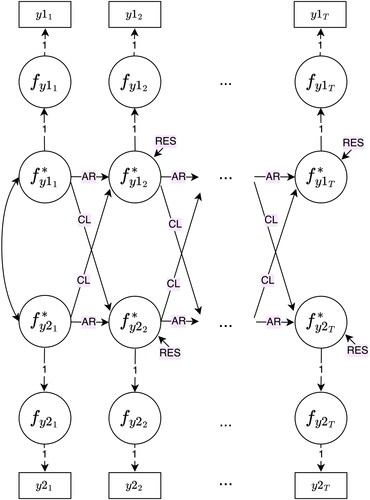
Figure B2. Factor cross-lagged panel model (fCLPM).

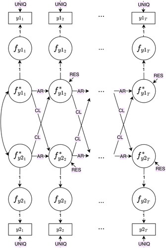
Figure B3. Random intercepts cross-lagged panel model (RI-CLPM).

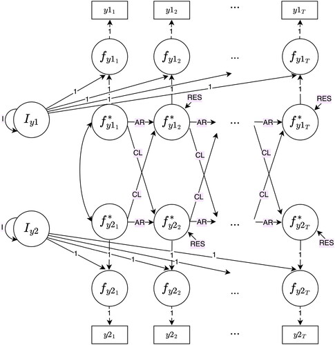
Figure B4. Stable trait autoregressive trait and state model (STARTS).

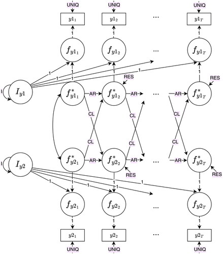
Figure B5. Latent curve model with structured residuals (LCM-SR).

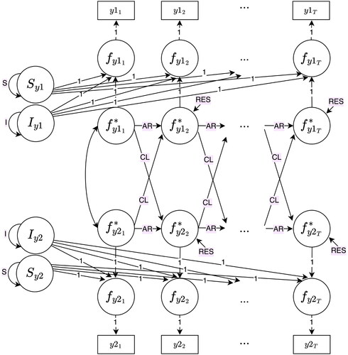
Figure B6. Autoregressive latent trajectory model (ALT).

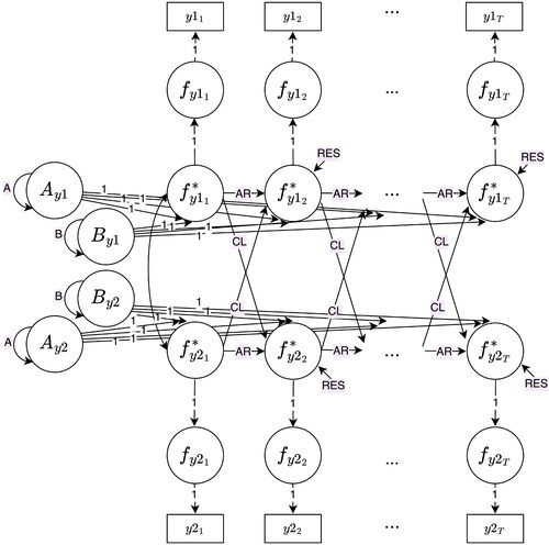
Figure B7. Latent change score model (LCS).

References

- Adolf, J. K., Loossens, T., Tuerlinckx, F., & Ceulemans, E. (2021). Optimal sampling rates for reliable continuous-time first-order autoregressive and vector autoregressive modeling. Psychological Methods, 26, 701–718. https://doi.org/10.1037/met0000398
- Allison, D. B. (1995). When is it worth measuring a covariate in a randomized clinical trial? Journal of Consulting and Clinical Psychology, 63, 339–343. https://doi.org/10.1037//0022-006x.63.3.339
- Allison, D. B., Allison, R. L., Faith, M. S., Paultre, F., & Pi-Sunyer, F. X. (1997). Power and money: Designing statistically powerful studies while minimizing financial costs. Psychological Methods, 2, 20–33. https://doi.org/10.1037/1082-989X.2.1.20
- Anderson, S. F., Kelley, K., & Maxwell, S. E. (2017). Sample-size planning for more accurate statistical power: A method adjusting sample effect sizes for publication bias and uncertainty. Psychological Science, 28, 1547–1562. https://doi.org/10.1177/0956797617723724
- Basagaña, X., & Spiegelman, D. (2010). Power and sample size calculations for longitudinal studies comparing rates of change with a time-varying exposure. Statistics in Medicine, 29, 181–192. https://doi.org/10.1002/sim.3772
- Basagaña, X., Xiaomei, L., & Spiegelman, D. (2011). Power and sample size calculations for longitudinal studies estimating a main effect of a time-varying exposure. Statistical Methods in Medical Research, 20, 471–487. https://doi.org/10.1177/0962280210371563
- Berry, D., & Willoughby, M. T. (2017). On the practical interpretability of cross-lagged panel models: Rethinking a developmental workhorse. Child Development, 88, 1186–1206. https://doi.org/10.1111/cdev.12660
- Bollen, K. A. (1989). Structural equations with latent variables. John Wiley & Sons.
- Bollen, K. A., & Curran, P. J. (2004). Autoregressive latent trajectory (ALT) models: A synthesis of two traditions. Sociological Methods & Research, 32, 336–383. https://doi.org/10.1177/0049124103260222
- Bolger, N., Stadler, G., & Laurenceau, J.-P. (2012). Power analysis for intensive longitudinal studies. In M. R. Mehl & T. S. Conner (Eds.), Handbook of research methods for studying daily life (pp. 285–301). The Guilford Press.
- Brockwell, P. J., & Davis, R. A. (2002). Introduction to time series and forecasting (2nd ed.). Springer.
- Brandmaier, A. M., von Oertzen, T., Ghisletta, P., Hertzog, C., & Lindenberger, U. (2015). LIFESPAN: A tool for the computer-aided design of longitudinal studies. Frontiers in Psychology, 6, 272. https://doi.org/10.3389/fpsyg.2015.00272
- Brandmaier, A. M., Ghisletta, P., & von Oertzen, T. (2020). Optimal planned missing data design for linear latent growth curve models. Behavior Research Methods, 52, 1445–1458. https://doi.org/10.3758/s13428-019-01325-y
- Champely, S. (2020). pwr: Basic functions for power analysis [Computer software] (version 1.3-0). https://cran.r-project.org/package=pwr
- Cole, D. A., Martin, N. C., & Steiger, J. H. (2005). Empirical and conceptual problems with longitudinal trait-state models: Introducing a trait-state-occasion model. Psychological Methods, 10, 3–20. https://doi.org/10.1037/1082-989X.10.1.3
- Cools, W., van den Noortgate, W., & Onghena, P. (2008). Ml-des: A program for designing efficient multilevel studies. Behavior Research Methods, 40, 236–249. https://doi.org/10.3758/BRM.40.1.236
- Crutzen, R., & Peters, G.-J Y. (2017). Targeting next generations to change the common practice of underpowered research. Frontiers in Psychology, 8, 1184. https://doi.org/10.3389/fpsyg.2017.01184
- Curran, P. J., & Bollen, K. A. (2001). The best of both worlds: Combining autoregressive and latent curve models. In L. M. Collins & A. G. Sayer (Eds.), New methods for the analysis of change (pp. 107–135). American Psychological Association. https://doi.org/10.1037/10409-004
- Curran, P. J. (2003). Have multilevel models been structural equation models all along? Multivariate Behavioral Research, 38, 529–569. https://doi.org/10.1207/s15327906mbr3804_5
- Curran, P. J., Howard, A. L., Bainter, S. A., Lane, S. T., & McGinley, J. S. (2014). The separation of between-person and within-person components of individual change over time: A latent curve model with structured residuals. Journal of Consulting and Clinical Psychology, 82, 879–894. https://doi.org/10.1037/a0035297
- Enders, W. (2015). Applied econometric time series. (4th ed.). Wiley.
- Faul, F., Erdfelder, E., Lang, A.-G., & Buchner, A. (2007). G*Power 3: A flexible statistical power analysis program for the social, behavioral, and biomedical sciences. Behavior Research Methods, 39, 175–191. https://doi.org/10.3758/BF03193146
- Fan, X. (2003). Power of latent growth modeling for detecting group differences in linear growth trajectory parameters. Structural Equation Modeling: A Multidisciplinary Journal, 10, 380–400. https://doi.org/10.1207/S15328007SEM1003_3
- Ferguson, T. S. (1996). A course in large sample theory. Springer. https://doi.org/10.1007/978-1-4899-4549-5
- Hertzog, C., Lindenberger, U., Ghisletta, P., & von Oertzen, T. (2006). On the power of multivariate latent growth curve models to detect correlated change. Psychological Methods, 11, 244–252. https://doi.org/10.1037/1082-989X.11.3.244
- Hertzog, C., von Oertzen, T., Ghisletta, P., & Lindenberger, U. (2008). Evaluating the power of latent growth curve models to detect individual differences in change. Structural Equation Modeling: A Multidisciplinary Journal, 15, 541–563. https://doi.org/10.1080/10705510802338983
- Hamagami, F., & McArdle, J. J. (2001). Advanced studies of individual differences: Linear dynamic models for longitudinal data analysis. In G. A. Marcoulides & R. E. Schumacker (Eds.), New developments and techniques in structural equation modeling (pp. 203–246). Psychology Press. https://doi.org/10.4324/9781410601858
- Hamaker, E. L., Kuiper, R. M., & Grasman, R. P. P. P. (2015). A critique of the cross-lagged panel model. Psychological Methods, 20, 102–116. https://doi.org/10.1037/a0038889
- Hamilton, J. D. (1994). Time series analysis (Vol. 2). Princeton University Press.
- Harrall, K. K., Muller, K. E., Starling, A. P., Dabelea, D., Barton, K. E., Adgate, J. L., & Glueck, D. H. (2023). Power and sample size analysis for longitudinal mixed models of health in populations exposed to environmental contaminants: A tutorial. BMC Medical Research Methodology, 23, 1–13. https://doi.org/10.1186/s12874-022-01819-y
- Hecht, M., Hardt, K., Driver, C. C., & Voelkle, M. C. (2019). Bayesian continuous-time Rasch models. Psychological Methods, 24, 516–537. https://doi.org/10.1037/met0000205
- Hecht, M., & Voelkle, M. C. (2021). Continuous-time modeling in prevention research: An illustration. International Journal of Behavioral Development, 45, 19–27. https://doi.org/10.1177/0165025419885026
- Hecht, M., & Zitzmann, S. (2020). A computationally more efficient Bayesian approach for estimating continuous-time models. Structural Equation Modeling: A Multidisciplinary Journal, 27, 829–840. https://doi.org/10.1080/10705511.2020.1719107
- Hecht, M., & Zitzmann, S. (2021). Exploring the unfolding of dynamic effects with continuous-time models: Recommendations concerning statistical power to detect peak cross-lagged effects. Structural Equation Modeling: A Multidisciplinary Journal, 28, 894–902. https://doi.org/10.1080/10705511.2021.1914627
- Iddi, S., & Donohue, M. C. (2022). Power and sample size for longitudinal models in R – The longpower package and Shiny app. The R Journal, 14, 264–282. https://doi.org/10.32614/RJ-2022-022
- Jak, S., Jorgensen, T. D., Verdam, M. G. E., Oort, F. J., & Elffers, L. (2021). Analytical power calculations for structural equation modeling: A tutorial and Shiny app. Behavior Research Methods, 53, 1385–1406. https://doi.org/10.3758/s13428-020-01479-0
- Kenny, D. A., & Zautra, A. (1995). The trait-state-error model for multiwave data. Journal of Consulting and Clinical Psychology, 63, 52–59. https://doi.org/10.1037/0022-006X.63.1.52
- Kenny, D. A., & Zautra, A. (2001). Trait-state models for longitudinal data. In L. M. Collins & A. G. Sayer (Eds.), New methods for the analysis of change (pp. 243–263). American Psychological Association.
- Lafit, G., Adolf, J. K., Dejonckheere, E., Myin-Germeys, I., Viechtbauer, W., & Ceulemans, E. (2021). Selection of the number of participants in intensive longitudinal studies: A user-friendly Shiny app and tutorial for performing power analysis in multilevel regression models that account for temporal dependencies. Advances in Methods and Practices in Psychological Science, 4. https://doi.org/10.1177/2515245920978738
- Lafit, G., Artner, R., & Ceulemans, E. (2023). Enabling analytical power calculations for multilevel models with autocorrelated errors through deriving and approximating the information matrix. PsyArXiv. https://doi.org/10.31234/osf.io/tj5bv
- Lafit, G., Sels, L., Adolf, J. K., Loeys, T., & Ceulemans, E. (2022). PowerLAPIM: An application to conduct power analysis for linear and quadratic longitudinal actor-partner interdependence models in intensive longitudinal dyadic designs. Journal of Social and Personal Relationships, 39, 3085–3115. https://doi.org/10.1177/02654075221080128
- Liu, G., & Liang, K.-Y. (1997). Sample size calculations for studies with correlated observations. Biometrics, 53, 937–947. https://doi.org/10.2307/2533554
- Lohmann, J. F., Zitzmann, S., Voelkle, M. C., & Hecht, M. (2022). A primer on continuous-time modeling in educational research: An exemplary application of a continuous-time latent curve model with structured residuals (CT-LCM-SR) to PISA data. Large-Scale Assessments in Education, 10, 32. https://doi.org/10.1186/s40536-022-00126-8
- Lu, K., Luo, X., & Chen, P.-Y. (2008). Sample size estimation for repeated measures analysis in randomized clinical trials with missing data. The International Journal of Biostatistics, 4, 9. https://doi.org/10.2202/1557-4679.1098
- Luhmann, M., Schimmack, U., & Eid, M. (2011). Stability and variability in the relationship between subjective well-being and income. Journal of Research in Personality, 45, 186–197. https://doi.org/10.1016/j.jrp.2011.01.004
- Lütkepohl, H. (2005). New introduction to multiple time series analysis. Springer.
- MacCallum, R. C., Browne, M. W., & Sugawara, H. M. (1996). Power analysis and determination of sample size for covariance structure modeling. Psychological Methods, 1, 130–149. https://doi.org/10.1037/1082-989X.1.2.130
- McArdle, J. J., & Hamagami, F. (2001). Latent difference score structural models for linear dynamic analyses with incomplete longitudinal data. In L. M. Collins & A. G. Sayer (Eds.), New methods for the analysis of change (pp. 137–175). American Psychological Association.
- McArdle, J. J. (2009). Latent variable modeling of differences and changes with longitudinal data. Annual Review of Psychology, 60, 577–605. https://doi.org/10.1146/annurev.psych.60.110707.163612
- Mebane, W. R., & Sekhon, J. S. (2011). Genetic optimization using derivatives: The rgenoud package for R. Journal of Statistical Software, 42, 1–26. https://doi.org/10.18637/jss.v042.i11
- Mehta, P. D., & Neale, M. C. (2005). People are variables too: Multilevel structural equations modeling. Psychological Methods, 10, 259–284. https://doi.org/10.1037/1082-989X.10.3.259
- Moerbeek, M. (2022). Power analysis of longitudinal studies with piecewise linear growth and attrition. Behavior Research Methods, 54, 2939–2948. https://doi.org/10.3758/s13428-022-01791-x
- Mulder, J. D., & Hamaker, E. L. (2021). Three extensions of the random intercept cross-lagged panel model. Structural Equation Modeling: A Multidisciplinary Journal, 28, 638–648. https://doi.org/10.1080/10705511.2020.1784738
- Muthén, B. O., & Curran, P. J. (1997). General longitudinal modeling of individual differences in experimental designs: A latent variable framework for analysis and power estimation. Psychological Methods, 2, 371–402. https://doi.org/10.1037/1082-989X.2.4.371
- Muthén, L. K., & Muthén, B. O. (2002). How to use a Monte Carlo study to decide on sample size and determine power. Structural Equation Modeling: A Multidisciplinary Journal, 9, 599–620. https://doi.org/10.1207/S15328007SEM0904_8
- Oberski, D. L. (2009). Jrule for Mplus [Computer software]. https://doi.org/10.5281/zenodo.10657
- R Core Team (2022). R: A language and environment for statistical computing. R Foundation for Statistical Computing. https://www.r-project.org
- Rao, C. R. (1973). Linear statistical inference and its applications (2nd ed.). Wiley.
- Raudenbush, S. W., et al. (2011). Optimal design software for multi-level and longitudinal research [Computer software]. http://hlmsoft.net/od
- Raudenbush, S. W., & Liu, X.-F. (2001). Effects of study duration, frequency of observation, and sample size on power in studies of group differences in polynomial change. Psychological Methods, 6, 387–401. https://doi.org/10.1037/1082-989X.6.4.387
- Ryan, O., Kuiper, R. M., & Hamaker, E. L. (2018). A continuous time approach to intensive longitudinal data: What, why and how? In K. van Montfort, J. H. L. Oud, & M. C. Voelkle (Eds.), Continuous time modeling in the behavioral and related sciences (pp. 27–57). Springer International Publishing. https://doi.org/10.1007/978-3-319-77219-6
- Saris, W. E., Satorra, A., & Van der Veld, W. M. (2009). Testing structural equation models or detection of misspecifications? Structural Equation Modeling: A Multidisciplinary Journal, 16, 561–582. https://doi.org/10.1080/10705510903203433
- Satorra, A., & Saris, W. E. (1985). Power of the likelihood ratio test in covariance structure analysis. Psychometrika, 50, 83–90. https://doi.org/10.1007/BF02294150
- Schlesselman, J. J. (1973). Planning a longitudinal study: II. Frequency of measurement and study duration. Journal of Chronic Diseases, 26, 561–570. https://doi.org/10.1016/0021-9681(73)90061-1
- Selig, J. P., & Little, T. D. (2012). Autoregressive and cross-lagged panel analysis for longitudinal data. In B. Laursen, T. D. Little, & N. A. Card (Eds.), Handbook of developmental research methods (pp. 265–278). The Guilford Press.
- Shumway, R. H., & Stoffer, D. S. (2015). Time series analysis and its applications (EZ Edition). Springer.
- Taylor, D. J., & Muller, K. E. (1995). Computing confidence bounds for power and sample size of the general linear univariate model. The American Statistician, 49, 43–47. https://doi.org/10.2307/2684810
- Taylor, D. J., & Muller, K. E. (1996). Bias in linear model power and sample size calculation due to estimating noncentrality. Communications in Statistics - Theory and Methods, 25, 1595–1610. https://doi.org/10.1080/03610929608831787
- Tekle, F. B., Tan, F. E. S., & Berger, M. P. F. (2011). Too many cohorts and repeated measurements are a waste of resources. Journal of Clinical Epidemiology, 64, 1383–1390. https://doi.org/10.1016/j.jclinepi.2010.11.023
- Usami, S., Hayes, T., & McArdle, J. J. (2015). On the mathematical relationship between latent change score and autoregressive cross-lagged factor approaches: Cautions for inferring causal relationship between variables. Multivariate Behavioral Research, 50, 676–687. https://doi.org/10.1080/00273171.2015.1079696
- Usami, S., Murayama, K., & Hamaker, E. L. (2019). A unified framework of longitudinal models to examine reciprocal relations. Psychological Methods, 24, 637–657. https://doi.org/10.1037/met0000210
- van Breukelen, G. J. P. (2013). Optimal experimental design with nesting of persons in organizations. Zeitschrift für Psychologie, 221, 145–159. https://doi.org/10.1027/2151-2604/a000143
- von Oertzen, T. (2010). Power equivalence in structural equation modelling. The British Journal of Mathematical and Statistical Psychology, 63, 257–272. https://doi.org/10.1348/000711009X441021
- von Oertzen, T., Ghisletta, P., & Lindenberger, U. (2010). Simulating power in latent growth curve modeling. In M. W. Crocker & J. Siekmann (Eds.), Resource-adaptive cognitive processes (pp. 95–117). Springer.
- von Oertzen, T., & Brandmaier, A. M. (2013). Optimal study design with identical power: An application of power equivalence to latent growth curve models. Psychology and Aging, 28, 414–428. https://doi.org/10.3758/s13428-013-0384-4
- Voelkle, M. C., Gische, C., Driver, C. C., & Lindenberger, U. (2018). The role of time in the quest for understanding psychological mechanisms. Multivariate Behavioral Research, 53, 782–805. https://doi.org/10.1080/00273171.2018.1496813
- Voelkle, M. C., & Oud, J. H. L. (2013). Continuous time modelling with individually varying time intervals for oscillating and non-oscillating processes: Continuous time modelling. The British Journal of Mathematical and Statistical Psychology, 66, 103–126. https://doi.org/10.1111/j.2044-8317.2012.02043.x
- Voelkle, M. C., Oud, J. H. L., Davidov, E., & Schmidt, P. (2012). An SEM approach to continuous time modeling of panel data: Relating authoritarianism and anomia. Psychological Methods, 17, 176–192. https://doi.org/10.1037/a0027543
- Wang, Y. A., & Rhemtulla, M. (2021). Power analysis for parameter estimation in structural equation modeling: A discussion and tutorial. Advances in Methods and Practices in Psychological Science, 4. https://doi.org/10.1177/2515245920918253
- Wu, W., Jia, F., Rhemtulla, M., & Little, T. D. (2016). Search for efficient complete and planned missing data designs for analysis of change. Behavior Research Methods, 48, 1047–1061. https://doi.org/10.3758/s13428-015-0629-5
- Zitzmann, S., Wagner, W., Lavelle-Hill, R., Jung, A., Jach, H., Loreth, L., Lindner, C., Schmidt, F. T. C., Edelsbrunner, P. A., Schaefer, C. D., Deutschländer, R., Schauber, S., Krammer, G., Wolff, F., Hui, B., Fischer, C., Bardach, L., Nagengast, B., Hecht, M., et al. (2023). On the role of variation in measures, the worth of underpowered studies, and the need for tolerance among researchers: Some more reflections on Leising (2022) from a methodological, statistical, and social-psychological perspective [Manuscript submitted for publication].
- Zitzmann, S., Wagner, W., Hecht, M., Helm, C., Fischer, C., Bardach, L., & Göllner, R. (2022). How many classes and students should ideally be sampled when assessing the role of classroom climate via student ratings on a limited budget? An optimal design perspective. Educational Psychology Review, 34, 511–536. https://doi.org/10.1007/s10648-021-09635-4