CAS FGOALS-f3-L model dataset descriptions for CMIP6 DECK experiments

ABSTRACT

The datasets of the Chinese Academy of Sciences (CAS) Flexible Global Ocean–Atmosphere–Land System (FGOALS-f3-L) model for the baseline experiment of the fully coupled runs in the Diagnostic, Evaluation and Characterization of Klima (DECK) common experiments of phase 6 of the Coupled Model Intercomparison Project (CMIP6) are described in this study. The CAS FGOALS-f3-L model team submitted the piControl run with a near equilibrium ocean state for 561 model years, and 160-year integrations for three ensemble members of abrupt-4× CO2 and 1pctCO2, respectively. The ensemble members restart from the 600, 650 and 700 model years in the piControl run, respectively. The baseline performances of the model are validated in this article. The preliminary evaluation suggests that the CAS FGOALS-f3-L model can preserve the long-term stability well for a mean net radiation flux of 0.31 W m⁻² at the top of the atmosphere, and a limited decreasing trend of −0.03 W m⁻²/100 yr. The global annual mean SST is 16.45°C for the 561-year mean, with an increase of 0.03°C/100 yr. The model captures the basic spatial patterns of climate-mean SST and precipitation, but still underestimates the SST over the warm pool. The coupled model mitigates the precipitation bias in the ITCZ compared with the results from CMIP5. Moreover, the model’s climate sensitivity represented by the equilibrium climate sensitivity has been reduced from 4.5°C in CMIP5 to 3.0°C in CMIP6. All these datasets contribute to the benchmark of model behaviors for the desired continuity of CMIP.

Graphical abstract

摘要

本文介绍了CAS FGOALS-f3-L参加CMIP6 DECK耦合试验数据。主要包括piControl, abrupt-4×CO2和1pctCO2的试验设计, 模式设置以及初步结果评估。piControl提供了561年的模拟结果, abrupt-4×CO2和1pctCO2分别提供了三组集合成员, 每个成员包括160年的积分。初步评估结果表明, piControl试验中, 耦合模式可以保证长期稳定积分。在气候态降水模拟上, piControl试验可以合理的再现全球海表温度和降水的基本分布型, 相比上一代耦合模式, 在ITCZ地区的降水有所改进。另一方面耦合模式的气候敏感度约为3.0°C, 相比上一代的耦合模式更为合理。

KEYWORDS:

• CMIP6
• DECK
• FGOALS-f3-L
• piControl
• abrupt-4×CO2
• 1pctCO2; climate sensitivity

关键词:

• 第六届国际耦合模式比较计划; DECK
• FGOALS-f3-L
• 工业革命前试验; 4倍二氧化碳试验; 1%每年二氧化碳试验
• 气候敏感度

1. Introduction

The identification of a handful of common experiments—the Diagnostic, Evaluation, and Characterization of Klima (DECK) experiments (klima is Greek for ‘climate’)— was proposed as the fundamental experiments in phase 6 of the Coupled Model Intercomparison Project (CMIP6) (Eyring et al. 2016). The DECK experiments are used to establish model characteristics and serve as the entry card for a model to participate in one of CMIP’s phases. DECK contains four baseline experiments: (a) a historical Atmospheric Model Intercomparison Project (amip) simulation; (b) a pre-industrial control simulation (piControl or esm-piControl); (c) a simulation forced by an abrupt quadrupling of CO₂ (abrupt-4×CO2); and (d) a simulation forced by a 1% yr⁻¹ CO₂ increase (1pctCO2). The amip experiment is forced by observed sea surface temperature (SST) and sea ice, while the other three experiments are the coupling of the atmospheric and oceanic circulation simulations. The goal of DECK is to make it possible to track changes in the performance and response of models and CMIP phases for consistency.

The Chinese Academy of Sciences (CAS) Flexible Global Ocean–Atmosphere–Land System model, finite-volume version 3 (CAS FGOALS-f3-L) (the ‘L’ denotes a low horizontal resolution of 100 km), climate system model was developed at the LASG (State Key Laboratory of Numerical Modeling for Atmospheric Sciences and Geophysical Fluid Dynamics), Institute of Atmospheric Physics (IAP), CAS (Bao and Li 2020). The model group recently completed the DECK simulations (in late 2019), and the model outputs have been released after a series of postprocesses on the Earth System Grid (ESG) node at the IAP. For the amip simulations, the datasets have already been published (in early 2019), and dataset descriptions are documented in He et al. (2019). The other three experiments—piControl, abrupt-4× CO2 and 1pctCO2—are to be introduced in this paper, since the model configurations are the same. The piControl simulation is performed under conditions of 1850, which is representative of the period before global industrialization. This simulation is an attempt to produce a stable quasi-equilibrium climate state under 1850 conditions for the other experiments, such as the historical simulation, abrupt-4×CO2, 1pctCO2, etc. It can also be used to study the unforced internal variability of the climate system. The abrupt-4×CO2 experiment is designed to understand the global surface temperature feedback responses to CO₂ forcing (Gregory et al. 2004), while the 1pctCO2 experiment is designed for studying model responses under simplified but somewhat more realistic forcing than abrupt-4×CO2 (Meehl et al. 2000).

The CAS FGOALS-f3-L model group has completed the above simulations and provides a description of the DECK experiment outputs—specifically, those of piControl, abrupt-4×CO2 and 1pctCO2—and the relevant essential model configurations and experimental methods for a variety of users in this paper. Section 2 describes the model and experimental design. Section 3 addresses the technical validation of the outputs from the CAS FGOALS-f3-L experiments. Section 4 provides usage notes, and section 5 presents a short summary.

2. Model and experiments

2.1 Introduction to the model

CAS FGOALS-f3-L is a climate system model. The model configuration is briefly listed in Table 1. The coupled model is composed of five components:

1. The Finite-volume Atmospheric Model (FAMIL), which has been updated from version 1 (Zhou et al. 2015) to version 2.2 (Li et al. 2019; Bao et al. 2019; Bao and Li 2020). The model dynamic core, physics packages, and baseline performance of the amip experiments are addressed in He et al. (2019).

2. Version 3 of the LASG/IAP Climate System Ocean Model (LICOM3) (Liu et al. 2012; Li et al. 2017). The updates from LICOM2 and the baseline performance of the model for the historical runs are presented in Guo et al. (2020)

3. Version 4.0 of the Community Land Model (CLM4) (Oleson et al. 2010).

4. Version 4 of the Los Alamos Sea Ice Model (CICE4) (Hunke et al. 2010).

5. Version 7 of the coupler from the National Center for Atmospheric Research (NCAR) (Craig, Vertenstein, and Jacob 2011).

Table 1. Model configurations of CAS FGOALS-f3-L

Model configuration	FGOALS-f3-L
Atmosphere	FAMILv2.2 Resolution: C96 (1° × 1°) L32 (Zhou et al. 2015; Bao et al. 2019; He et al. 2019; Li et al. 2019)
Ocean	LICOM3 Resolution: Triple grid (1° × 1°) L30 (Liu et al. 2012; Li et al. 2017;)
Land	CLM4.0 Resolution: 1° × 1° (Lawrence et al. 2011)
Sea ice	CICE4.0 Resolution: 1° × 1° (Hunke et al. 2010)
Coupler	NCAR Coupler7 (Craig, Vertenstein, and Jacob 2011)

2.2 Descriptions of experiments

The experiment settings of piControl, abrupt-4× CO2 and 1pctCO2 are introduced here. The basic configurations of these three simulations are summarized in Table 2. For piControl, the external forcings are prescribed as their values in 1850 (Table 3). The global annual mean greenhouse gas (GHG) concentrations are from Meinshausen et al. (2017). The solar irradiance is fixed at 1360.8 W m⁻² (Matthes et al. 2017). The 3D ozone concentrations are from http://blogs.reading.ac.uk/ccmi/forcing-databases-in-support-of-cmip6/. The aerosol mass concentrations are also prescribed and taken from the NCAR Community Atmosphere Model with Chemistry (CAM-Chem) (Lamarque et al. 2012), including sulfates, sea salt, black carbon, organic carbon, and dust. The piControl experiment runs for 1160 model years, with the first 599 years used as spin-up time. The model outputs from model-year 600 to 1160 are submitted as the quasi-equilibrium state for the fully coupled model.

Table 2. Experiment designs

experiment_id	Variant_label	Restart time	Years of integration	Experiment design	DOI for experiment_id
piControl	r1i1p1f1	600	561	Free coupled model run with all the external forcings fixed as their values in 1850. The first 599 years of integration are taken as the spin-up time and the model outputs after 600 model years are submitted.	http://doi.10.22033/ESGF/CMIP6.3447
abrupt-4×CO2	r1i1p1f1	600	160	Restart run from 1 January in model-year 600 of piControl. CO2 prescribed as four times that in piControl. All other external forcings identical to piControl.	http://doi.10.22033/ESGF/CMIP6.3176
	r2i1p1f1	650	160	Same as r1i1p1f1 but with a restart from 1 January in model-year 650 of piControl.
	r3i1p1f1	700	160	Same as r1i1p1f1 but with a restart from 1 January in model-year 700 of piControl.
1pctCO2	r1i1p1f1	600	160	Restart run from 1 January in model-year 600 of piControl. CO2 prescribed to increase 1% yr^−1. All other external forcings identical to piControl.	http://doi.10.22033/ESGF/CMIP6.3054
	r2i1p1f1	650	160	As in r1i1p1f1 but with a restart from 1 January in model-year 650 of piControl.
	r3i1p1f1	700	160	As in r1i1p1f1 but with a restart from 1 January in model-year 700 of piControl.

Table 3. External forcing settings in piControl, abrupt-4×CO2, and 1pctCO2

External forcing	Description
GHGs	Fixed as their global mean values in 1850: CO2: 284.3 ppm in piControl 1137.2 ppm in abrupt-4×CO2 1% yr^−1 increase from 284.3 ppm in 1pctCO2 CH4: 808.2 ppb N2O: 273.0 ppb CFC-11 equivalent: 0.032 ppb CFC-12 equivalent: 0.016 ppb
Solar irradiance	1360.8 W m^−2
Aerosols	Three-dimensional distributions prescribed as their values in 1850, including sulfates, sea salt, black carbon, organic carbon, and dust (Lamarque et al. 2012)
Ozone	Three-dimensional distributions prescribed as their values in 1850 (http://blogs.reading.ac.uk/ccmi/forcing-databases-in-support-of-cmip6/)

The abrupt-4×CO2 experiments run for 160 years. The external forcings are the same as in piControl except that the CO₂ concentration is four times that of piControl. The time-lag method is used to realize the three perturbations that are identified by the variant_label: r1i1p1f1, r2i1p1f1, and r3i1p1f1. The characteristics in r1i1p1f1 denote the realization_index, initialization_index, physics_index, and forcing_index. The first experiment (r1i1p1f1) restarts from 1 January in model-year 600 of piControl. The second experiment (r2i1p1f1) is the same as r1i1p1f1 except that the integration restart date is 1 January in model-year 650. Similarly, the start date is 1 January in model-year 700 in the third experiment (r3i1p1f1).

The 1pctCO2 experiments are also integrated for 160 years. The external forcings are the same as in piControl except that the CO₂ concentration is increasing at 1% yr⁻¹. The ensemble method is the same as in abrupt-4×CO2, with restart dates for r1i1p1f1, r2i1p1f1 and r3i1p1f1 of 1 January in model-years 600, 650, and 700 in piControl, respectively. All of the DECK experiments documented in this paper have been officially published at the ESG node and the DOIs (digital object identifiers) for the experiment_id are listed in Table 2.

3. Basic performance of model results

The basic performances of the model simulations are evaluated in this section. As the external forcings are prescribed and held constant in the piControl experiment, the simulation mainly shows an internal climate variability for global climate. This simulation aims to provide a near-equilibrium ocean state and to serve as the control run for the other experiments. We show the global annual mean net radiation at top of the atmosphere (TOA) from model-years 600 to 1160 in Figure 1(a) to investigate the model’s stability. The result shows that the TOA net radiation is quite stable during the long-term integration, with a mean value of 0.31 W m⁻². The climate trend of the radiation is −0.03 W m⁻²/100 yr and the standard deviation is 0.37 W m⁻², which is also reasonable. In response to the TOA net radiation, the global annual mean SST shows a slight increasing climate trend of 0.03°C/100 yr (Figure 1(b)). The time series of SST is also quite stable, with a standard deviation of 0.11°C and mean value of 16.45, which are within the ranges of the CMIP5 climate models (Gupta et al. 2013). All these results suggest that the climate drift of CAS FGOALS-f3-L is small and the 561-year near-equilibrium ocean state in piControl is stable.

Figure 1. (a) Time series of global mean TOA net radiation (units: W m⁻²) for piControl from model-year 600 to 1160 with a global mean value of 0.31 W m⁻², standard deviation of 0.37 W m⁻² and climate trend of −0.03 W m⁻²/100 yr. (b) Time series of global mean SST for piControl from model-year 600 to 1160 with a global mean value of 16.45°C, standard deviation of 0.11°C and climate trend of 0.03°C/100 yr

The basic spatial characteristics of the climate-mean SST and precipitation for piControl are also examined, in Figure 2. Compared to the observed (Taylor, Williamson, and Zwiers, 2000) climate-mean (1871–1900) SST distribution (Figure 2(a)), CAS FGOALS-f3-L (Figure 2(b)) captures the large-scale pattern for the global meridional variations well. However, for the 28°C isothermal line, the model underestimates the SST, mainly over the western Pacific regions. This systematic bias persists from the previous version (see Figure 1 in Bao et al. (2013)). The simulated climate-mean precipitation is shown in Figure 3. Compared to the observation (Figure 2(a)) derived from Global Precipitation Climatology Project (Adler et al. 2003), the model reproduces the basic pattern both in the tropical and subtropical ocean regions. The most striking improvement is that the model largely overcomes the double ITCZ problem that existed in the previous version, characterized as the dry area (< 4 mm d⁻¹) over the equator close to the date line in FGOALS-f3-L (Figure 3(b)), but extending west to the Maritime Continent in the previous version (see Figure 5 in Bao et al. (2013)). However, the model still overestimates the precipitation over ocean regions while underestimating the precipitation over land. In particular, the precipitation over South American land is missing (Figure 3(b)). This bias also exists in the amip simulation (He et al. 2019), which implies that the land–air interactions are important for reproducing this pattern.

Figure 2. Climate mean distribution of SST (units: °C): (a) observation (1871–1900 mean); (b) FGOALS-f3-L (600–1160 mean)

Figure 3. Climate mean distribution of precipitation (units: mm d⁻¹): (a) observation (1979–2014); (b) FGOALS-f3-L (600–1160 mean)

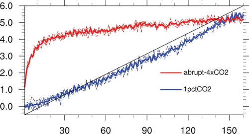
The abrupt-4×CO2 and 1pctCO2 experiments are designed to understand the climate feedback and to quantitatively estimate the model climate sensitivity. In general, the feedback response is measured by the global surface temperature change under imposed CO₂ forcing. In 1pctCO2, the CO₂ increases at a rate of 1% yr⁻¹, staring from its 1850 value that is prescribed in piControl. The model responses to this forcing would be more realistic than in abrupt-4×CO2 (Meehl et al. 2000). For abrupt-4×CO2, the CO₂ concentration is quadrupled from its prescribed level in piControl and held fixed. In this experiment, the climate system subsequently evolves to a new equilibrium, and the net radiation flux at the TOA and the associated changes in surface air temperature (SAT) can be used to measure the model’s effective equilibrium climate sensitivity (ECS) (Gregory et al. 2004). We show the time series of the global annual mean SAT anomalies (relative to piControl) for both abrupt-4×CO2 and 1pctCO2 in Figure 4. The results from the ensemble members are shown as dashed lines while the ensemble means are shown as the thick solid lines. It is clear that the SAT increases gradually from 0 to 5.09°C in 1pctCO2 for the 150 years (Table 4). On the other hand, the SAT increases rapidly in abrupt-4×CO2 for the first 20 years to almost 4°C, reaching a near equilibrium state after 20 years and 5.07°C after 150 years of integration (Table 4). This result suggests the model’s climate sensitivity is lower than in its last version, as documented in Chen, Zhou, and Guo (2014), for the SAT increases to almost 6°C in both simulations. Following Gregory et al. (2004), the ECS of CAS FGOALS-f3-L is estimated in Figure 5. It shows that the results within the three ensemble members are close to each other and the ensemble mean ECS appears at 3.03°C, which is lower than in the previous version (4.5°C) as documented in Chen, Zhou, and Guo (2014). This improvement is mainly due to the changes in the radiation and microphysics schemes in the atmospheric model, such that the unrealistic greenhouse effect over the upper tropical troposphere can be reasonably handled (He 2016). The model’s reasonable climate sensitivity also contributes to the realistic simulations of the historical run as documented in Guo et al. (2020).

Table 4. Surface air temperature responses to abrupt quadrupling of CO₂ and 1% yr⁻¹ CO₂ increase at 150 model years

SAT responses (°C) at 150 model years	abrupt-4×CO2	1pctCO2
Ensemble mean	5.07	5.09
r1i1p1f1	5.20	5.16
r2i1p1f1	4.98	5.18
r3i1p1f1	5.04	4.95

Figure 4. Time series of global mean surface air temperature anomalies (units: °C; relative to piControl) for ensemble means of abrupt-4×CO2 and 1pctCO2, respectively. The dashed lines are the three ensemble members, respectively

Figure 5. Climate sensitivity of CAS FGOALS-f3-L estimated from the 160-year integrations from abrupt-4×CO2 and associated piControl simulations. The abscissa is the surface air temperature anomaly (units: °C) and the vertical axis is the TOA net radiation anomaly (units: W m⁻²). The blue dashed lines are the extension lines of the regression lines. (a) r1i1p1f1; (b) r2i1p1f1; (c) r3i1p1f1; (d) ensemble mean

4. Usage notes

The original atmospheric model grid is in the cube–sphere grid system with a resolution of C96, which has six tiles and is irregular in the horizonal direction. We merged and interpolated the tiles to a nominal resolution of 1° on a global latitude–longitude grid, scaled by one-order conservation interpolation, for public use.

The format of datasets is version 4 of the Network Common Data Form (NetCDF), which can be easily read and written by common professional software such as Climate Data Operators (https://www.unidata.ucar.edu/software/netcdf/workshops/2012/third_party/CDO.html), netCDF Operator (http://nco.sourceforge.net), NCAR Command Language (http://www.ncl.ucar.edu), and Python (https://www.python.org).

5. Summary

The CAS FGOALS-f3-L model team has completed integrations of the CMIP6 DECK experiments including the piControl run with a near equilibrium ocean state for 561 model years, and 160-year integrations for three ensemble members of abrupt-4× CO2 and 1pctCO2, respectively. The climate trend of TOA net radiation fluxes in piControl is −0.03° W m⁻²/100 yr and the SST trend is 0.03°C/100 yr. The global annual mean SST is 16.45°C for the 561-year mean, with an increase of 0.03°C/100 yr. The estimated ECS for CAS FGOALS-f3-L is 3.0°C.

Acknowledgments

We would like to thank the editor and two anonymous reviewers for their constructive suggestions that helped to improve the overall quality of the manuscript.

Data availability statement

The data that support the findings of this study are available from https://esgf-node.llnl.gov/projects/cmip6/

Disclosure statement

No potential conflict of interest was reported by the authors.

Additional information

Funding

The research presented in this paper was jointly funded by the National Key Research and Development Program of China [grant number 2017YFA0604004], the National Natural Science Foundation of China [grant numbers 41530426, 91737306, U1811464, 91837101, 41730963, and 91958201], and the Strategic Priority Research Program of the Chinese Academy of Sciences [grant numbers XDA19060102 and XDB40030205].

References

- Adler, R. F., G. J. Huffman, A. Chang, R. Ferraro, P. P. Xie, J. Janowiak, B. Rudolf, et al. 2003. “The Version 2 Global Precipitation Climatology Project (GPCP) Monthly Precipitation Analysis (1979-Present)”. Journal of Hydrometeors 4: 1147–1167. doi:10.1175/1525-7541(2003)004<1147:TVGPCP>2.0.CO;2.
- Bao, Q., and J. Li. 2020. “Recent Progress in Climate Modeling of Precipitation over the Tibetan Plateau.” National Science Review. nwaa006. doi:10.1093/nsr/nwaa006.
- Bao, Q., P. F. Lin, T. J. Zhou, Y. M. Liu, Y. Q. Yu, G. X. Wu, B. He, et al. 2013. “The Flexible Global Ocean-atmosphere-land System Model, Spectral Version 2: FGOALS-s2.” Advances in Atmospheric Sciences 30 (3): 561–576. doi:10.1007/s00376-012-2113-9.
- Bao, Q., X. F. Wu, J. X. Li, L. Wang, B. He, X. C. Wang, Y. M. Liu, and G. X. Wu. 2019. “Outlook for ElNino and the Indian Ocean Dipole in Autumn-winter 2018–2019.” (In Chinese). Chinese Science Bulletin 64 (1): 73–78. doi:10.1360/N972018-00913.
- Chen, X. L., T. J. Zhou, and Z. Guo. 2014. “Climate Sensitivities of Two Versions of FGOALS Model to Idealized Radiative Forcing.” Science China: Earth Sciences 57: 1363–1373. doi:10.1007/s11430-013-4692-4.
- Craig, A., M. Vertenstein, and R. Jacob. 2011. “A New Flexible Coupler for Earth System Modeling Developed for CCSM4 and CESM1.” International Journal of High Performance Computing Applications 26: 31–42. doi:10.1177/1094342011428141.
- Eyring, V., S. Bony, G. A. Meehl, C. A. Senior, B. Stevens, R. J. Stouffer, and K. E. Taylor. 2016. “Overview of the Coupled Model Intercomparison Project Phase 6 (CMIP6) Experimental Design and Organization.” Geoscientific Model Development 9: 1937–1958. doi:10.5194/gmd-9-1937-2016.
- Gregory, J. M., W. J. Ingram, M. A. Palmer, G. S. Jones, P. A. Stott, R. B. Thorpe, J. A. Lowe, T. C. Johns, and K. D. williams. 2004. “A New Method for Diagnosing Radiative Forcing and Climate Sensitivity.” Geophysical Research Letters 31: L03205. doi:10.1029/2003gl018747.
- Guo, Y., Y. Q. Yu, P. F. Lin, H. L. Liu, B. He, Q. Bao, S. W. Zhao, and X. W. Wang. 2020. “Overview of the CMIP6 Historical Experiment Datasets with the Climate System Model CAS FGOALS-f3-L.” Advances in Atmosphere Science 37 12. (in press). doi:10.1007/s00376-020-2004-4.
- Gupta, A. S., N. C. Jourdain, J. N. Brown, and D. Monselesan. 2013. “Climate Drift in the CMIP5 Models.” Journal of Climate 26 (21): 8597–8615. doi:10.1175/JCLI-D-12-00521.1.
- He, B. 2016. “Unrealistic Treatment of Detrained Water Substance in FGOALS-s2 and Its Influence on the Model’s Climate Sensitivity.” Atmospheric and Oceanic Science Letters 9 (1): 45–51. doi:10.1080/16742834.2015.1124601.
- He, B., Q. Bao, X. C. Wang, L. J. Zhou, X. F. Wu, Y. M. Liu, G. X. Wu, et al. 2019. “CAS FGOALS-f3-L Model Datasets for CMIP6 Historical Atmospheric Model Intercomparison Project Simulation.” Advances in Atmospheric Sciences 36 (8): 771–778. doi:10.1007/s00376-019-9027-8.
- Hunke, E. C., W. H. Lipscomb, A. K. Turner, N. Jeffery, and S. Elliott. 2010. “CICE: The Los Alamos Sea Ice Model Documentation and Software User’s Manual Version 4.1 LA-CC-06-012.” T-3 Fluid Dynamics Group, Los Alamos National Laboratory, 675.
- Lamarque, J.-F., L. K. Emmons, P. G. Hess, D. E. Kinnison, S. Tilmes, F. Vitt, C. L. Heald, et al. 2012. “CAM-chem: Description and Evaluation of Interactive Atmospheric Chemistry in the Community Earth System Model.” Geoscientific Model Development 5 (2): 369–411. doi:10.5194/gmd-5-369-2012.
- Lawrence, D. M., K. W. Oleson, M. G. Flanner, P. E. Thornton, S. C. Swenson, P. J. Lawrence, X. B. Zeng, et al. 2011. “Parameterization Improvements and Functional and Structural Advances in Version 4 of the Community Land Model.” Journal of Advances in Modeling Earth Systems. 3: M03001. doi:10.1029/2011MS00045.
- Li, J. X., Q. Bao, Y. M. Liu, G. X. Wu, L. Wang, B. He, X. C. Wang, and J. D. Li. 2019. “Evaluation of FAMIL2 in Simulating the Climatology and Seasonal-to-interannual Variability of Tropical Cyclone Characteristics.” Journal of Advances in Modeling Earth Systems. doi:10.1029/2018MS001506.
- Li, X., Y. Yu, H. Liu, and P. Lin. 2017. “Sensitivity of Atlantic Meridional Overturning Circulation to the Dynamical Framework in an Ocean General Circulation Model.” Journal of Meteorological Research 31: 490–501. doi:10.1007/s13351-017-6109-3.
- Liu, H., P. Lin, Y. Yu, and X. Zhang. 2012. “The Baseline Evaluation of LASG/IAP Climate System Ocean Model (LICOM) Version 2.” Acta Meteorologica Sinica 26: 318–329. doi:10.1007/s13351-012-0305-y.
- Matthes, K., B. Funke, M. E. Andersson, L. Barnard, J. Beer, P. Charbonneau, M. A. Clilverd, et al. 2017. “Solar Forcing for CMIP6 (V3. 2).” Geoscientific Model Development 10 (6): 2247–2302. doi:10.5194/gmd-10-2247-2017.
- Meehl, G. A., G. J. Boer, C. Covey, M. Latif, and R. J. Stouffer. 2000. “The Coupled Model Intercomparison Project (CMIP).” Bulletin of the American Meteorological Society 81 (2): 313–318. doi:10.1175/1520-0477(2000)081<0313:TCMIPC>2.3.CO;2.
- Meinshausen, M., E. Vogel, A. Nauels, K. Lorbacher, N. Meinshausen, D. M. Etheridge, P. J. Fraser, et al. 2017. “Historical Greenhouse Gas Concentrations for Climate Modelling (CMIP6).” Geoscientific Model Development 10 (5): 2057–2116. doi:10.5194/gmd-10-2057-2017.
- Oleson, K. W., D. M. Lawrence, G. B. Mark, B. Gordon, M. G. Flanner, K. Erik, L. Samuel, et al. 2010. “Technical Description of Version 4.0 Of the Community Land Model (CLM).” NCAR/TN–461 + STR, 173
- Taylor, K. E., D. Williamson, and F. Zwiers. 2000. The Sea Surface Temperature and Sea Ice Concentration Boundary Conditions for AMIP II Simulations. PCMDI Report 60, Program for Climate Model Diagnosis and Intercomparison, Lawrence Livermore National Laboratory, 25.
- Zhou, L., Q. Bao, Y. M. Liu, G. X. Wu, W. C. Wang, X. C. Wang, B. He, H. Y. Yu, and J. D. Li. 2015. “Global Energy and Water Balance: Characteristics from Finite‐volume Atmospheric Model of the IAP/LASG (FAMIL1).” Journal of Advances in Modeling Earth Systems 7 (1): 1–20. doi:10.1002/2014ms000349.