Forecasting cauliflower prices in Nepal: a comparative analysis using seasonal time series and nonlinear models

Abstract

This study aims to examine the seasonal price trends of cauliflower in the Nepalese market over the past decade, considering its significance as a major vegetable in terms of production and land area. The primary goal is to predict short-term market prices using econometric time-series analysis and artificial neural networks (ANNs), providing valuable insights for stakeholders, such as farmers, policymakers, researchers and students to make informed decisions and implement effective strategies for production, marketing, and distribution. The data, derived from the annual reports of the Kalimati Fruits and Vegetable Market covering April 2013 to March 2023, serves as the foundation for the analysis. Utilising the Seasonal Auto-Regressive Integrated Moving Average (SARIMA), Long Short-Term Memory Recurrent Neural Network (LSTM RNN) and Facebook (Fb) Prophet models, the study probes into the intricate seasonal patterns and trends in cauliflower prices. In contrast to conventional literature trends, the results of this study highlight the superior forecast accuracy of the SARIMA model, sizing the need for tailored-modeling approaches to address the complexities of the agricultural commodity market. The findings reveal an overall stable price structure in Nepal, implying the necessity for strategic planning to address potential challenges for cauliflower growers. The study recommends off-season cultivation to manage supply-demand imbalances during peak periods, enabling farmers to optimise profits and promote sustainable agricultural practices using policy interventions.

Keywords:

• Cauliflower prices
• SARIMA
• time series analysis
• LSTM RNN
• Fb Prophet model
• forecasting

REVIEWING EDITOR:

• Manuel Tejada, Universidad de Sevilla, Spain

SUBJECTS:

• Agriculture & Environmental Sciences
• Agriculture and Food
• Agriculture
• Econometrics
• Economic Forecasting

Introduction

Agriculture constitutes the backbone of the Nepalese economy, providing employment to approximately two-thirds of the country’s population and contributing 24% to the national GDP (MoALD, 2023). The cultivation and trade of vegetables are progressively gaining significance as a pivotal sub-sector contributing significantly to the nation’s economy in Nepal. Over the past decade, from 2012/2013 to 2021/2022, there has been a notable 18% increase in the area dedicated to vegetable crops, accompanied by a substantial 26% rise in production (MoALD, 2023). Regarding exports, vegetables rank as the fifth most crucial agricultural commodity, following lentils, cardamom, wheat and tea. However, the quantity of vegetables exported remains substantially lower than the amount imported in Nepal. In the fiscal year 2022/23, Nepal imported edible vegetables, certain roots and tubers, and planting materials amounting to NPR. Of 31,872.48 million and exported them worth NPR. 745.97 million, resulting in a trade deficit of NPR. Of −31,126.51 million (Department of Customs, Government of Nepal, 2023). This data underscores the considerable potential for increasing exports and reducing vegetable imports by maximising domestic production. The escalating demand for vegetables is further fueled by the rising income of the population, leading to a shift in dietary preferences from cereals to increased consumption of fruits and vegetables (Ghimire et al., 2018).

Nepal, characterised by a diverse range of agro-ecological variations, presents comparative advantages for the production and marketing of various vegetables. This diversity allows for the cultivation of a wide array of seasonal and off-season vegetables across the country, offering significant benefits to diet, nutrition, employment and the national economy. Vegetable production is distributed across Terai, Mid-hill and High hills, constituting 55%, 40% and 5%, respectively. Notably, cauliflower takes the lead as the most cultivated vegetable crop in Nepal, holding the number one position in terms of production area, covering 39,214 hectares, and production, reaching 61,015 metric tons (MoALD, 2023). Following closely, cabbage is another significant vegetable crop. The expansion of vegetable farming in Nepal can be attributed to the prospect of higher and earlier returns, even with relatively low investments.

Cauliflower, belonging to the Brassicaceae family, is a significant cruciferous vegetable crop known for its nutritional value and health benefits. It is rich in carbohydrates, proteins, fats, minerals, and vitamins and its consumption has been linked to a reduced risk of various diseases (Petruzzello, 2024). In Nepal, cauliflower holds great importance as a cold-weather vegetable, with favorable climatic and geographical conditions allowing for year-round production in different seasons. However, despite its production potential, cauliflower cultivation faces challenges related to poor production practices and marketing issues (MoALD, 2020).

The vegetable production sector, including cauliflower, is becoming increasingly significant in Nepal’s GDP contribution. However, there is a lack of comprehensive studies on vegetable production, marketing, and the economic dynamics faced by farmers, leading to limited information available for policy formulation (CASA, 2020). Therefore, conducting research from a systems perspective to understand the farm performance, production methods, inputs, productivity, market dynamics, seasonality analysis and profitability of cauliflower cultivation in specific areas is crucial (Poudel, 2019). The primary objective of this study is to analyse price trends (including seasonality and cyclical components) in the cauliflower market over the past 10 years, examine the seasonal price disparities and comprehend the overall market dynamics. By employing econometric time-series analysis as well as recent developments in the ANNs, the study aims to forecast short-term price movements to provide useful information for farmers, policymakers, researchers and students involved in this sector. This research intends to disseminate valuable insights to the stakeholders that will assist them in making informed decisions and implementing effective strategies to navigate the cauliflower market successfully.

Forecasting accurate and precise outcomes in complex systems involving policymakers and consumers can be a challenging task due to the intricate relationships among influential factors. While current methods primarily focus on qualitative analysis, there is a growing need for a quantitative forecasting approach. Among the commonly used time series models, the ARIMA model stands out as one of the most popular and in-demand (Alibuhtto & Ariyarathna, 2019; Adebiyi et al., 2014; Esther & Magdaline, 2017; Kaur & Ahuja, 2019). The ARIMA model incorporates autoregressive (AR), moving average (MA) and autoregressive moving average (ARMA) subclasses. Additionally, the seasonal ARIMA (or SARIMA) model has demonstrated considerable success in forecasting seasonal time series (Box et al., 2015; Kihoro et al., 2004).

In dealing with volatile data and price predictions, models from the GARCH family, such as GARCH, APARCH, TGARCH and EGARCH, have proven to be more effective. These models account for linear and nonlinear effects, providing improved forecasts. Hybrid models, which combine different forecasting techniques, have also shown promise in price forecasting (Rahman et al., 2023; Shet et al., 2022).

While some studies have explored the application of artificial neural networks (ANNs) and genetic algorithms in forecasting, they often overlook the production period. In recent years, there has been a modest increase in the utilisation of ANNs for time series forecasting (Kaur & Ahuja, 2019). Various ANN models, such as multilayered perceptions (MLP), feed forward network (FNN), time-lagged neural network (TLNN) and seasonal artificial neural network (SANN), have been developed and employed (Hamzacebi, 2008; Kamruzzaman et al., 2006). These models offer alternative approaches to forecasting and can provide exquisite intuition into different forecasting scenarios.

Several studies have explored the use of LSTM RNN for forecasting various environmental factors, such as wind, precipitation and humidity. Some researchers have replaced LSTM with GRU, achieving lower RMSE and MAE. Other works have compared LSTM with feed-forward neural networks (FFNNs), with some demonstrating improved forecast performance for groundwater tables and soil water tension. Additionally, the application of long- and short-term time series networks has been shown to effectively address both linear and non-linear structures in commodity price datasets, outperforming average baseline methods (Ouyang et al., 2019). More recent studies suggest that Fb Prophet demonstrates superior forecasting accuracy and computational efficiency compared to SARIMA and ETS. These findings underscore the significance of employing advanced time series forecasting techniques in the food industry to improve inventory management and reduce food wastage (Majhi et al., 2023).

Various forecasting models have been extensively utilised in contemporary studies (Hernandez-Matamoros et al., 2020). Literature offers a range of methods to predict the supply and prices of agricultural commodities, encompassing statistical models and machine learning models. The price of a product fluctuates based on its demand, which in turn is influenced by consumer willingness to purchase, often dependent on the product’s price. In the case of perishable horticultural produce, sellers must ensure the sale of their entire stock before the goods deteriorate (Le et al., 2019; Rohith et al., 2020).

Table 1 provides a comprehensive overview of the existing literature, presenting a wide array of models used for agricultural commodity price prediction. However, it is essential to note that these models often face challenges when applied to the horticultural sector due to its distinct characteristics, including high seasonality and limited product lifespan. While the table includes models, such as regression, decision trees, ANN, KNN, ARIMA and RNN, each excelling in various aspects, they may fall short in addressing the unique demands of horticultural price forecasting. Considering this, our study introduces Fb Prophet, LSTM RNN and SARIMA models, specifically tailored to tackle the intricacies of horticultural commodity price prediction. By incorporating these advanced approaches, we aim to provide more accurate and effective forecasts for the horticultural sector.

Table 1. Review of related work.

Author	Commodity	Forecasting model
Geweke and Porter-Hudak (1983)	Postwar monthly economic time series	Logarithmic Periodogram
Wang et al. (2011)	Household food	ARIMA
Yercan and Adanacioglu (2012)	Tomato	SARIMA (1,0,0) (1,1,1)12
Luo et al. (2013)	Cucumber	SARIMA (1,0,1) (1,1,1)12
da Veiga et al. (2014)	Dairy products	ARIMA, Holt-Winters
Choudhury and Jones (2014)	Crop yield	ARMA
Otu et al. (2014)	Inflation Rate	SARIMA
Arunraj et al. (2016)	Food consumption	SARIMA
Sellam and Poovammal (2016)	Rice	Regression Analysis
Souza et al. (2016)	Soybean	SARIMA
Esther and Magdaline (2017)	Pulses	ARIMA
Zhang et al. (2018)	Soybean	QR-RBF Neural Network
Bisht and Kumar (2019)	Pulses	GARCH
Vibas and Raqueno (2019)	Fruit, vegetable	ARIMA, SARIMA, ARIMAX
Mutwiri et al. (2019)	Tomato	SARIMA
Selvanayagam et al. (2019)	Vegetable	LSTM RNN, ARIMA
Rajeswari and Suthendran (2019)	Crop price	Hybrid Association rule-based Decision Tree (HADT)
Zahara et al. (2019)	Consumer price index	Nesterov Adam Optimization Algorithm
Wamalwa and Muchemi (2020)	Maize	SARIMA, ETS
Divisekara et al. (2021)	Red lentils	SARIMA (2,1,2) (0,1,1)52
Christensen et al. (2021)	Food crises	Logistic Regression, Neural Network
Purohit et al. (2021)	Agricultural crop prices	ARIMA, ETS, SVM, MLP, LSTM
Sarangi et al. (2021)	Consumer food price index	Backpropagation learning-based ANN
Oswari et al. (2022)	Food crop farmer index price	ARIMA, LSTM
Deléglise et al. (2022)	Financial services indicators	Machine Learning Techniques
Guo et al. (2022)	Price	AttLSTM-ARIMA-BP Model
Majhi et al. (2023)	Food price index	SARIMA, ETS, Fb Prophet
Giri and Giri (2023)	Cucumber	SARIMA, SSES

The price of cauliflower in Nepal is significantly influenced by seasonal variations, particularly during its specific growing season from January to March (AEC, 2006). These seasonal dynamics highlight the need for a thorough investigation into the price fluctuations of cauliflower to achieve accurate forecasting. By understanding the unique patterns and fluctuations associated with the seasonal variations, the forecasting models can be tailored accordingly to capture the dynamics of cauliflower prices and provide reliable predictions. The SARIMA model, specifically designed for time series data, is well-suited to capture the seasonal effect in cauliflower price trends. On the other hand, the application of ANN requires careful modifications to adapt it to time series data, as it is originally designed for cross-sectional data. While ANN may provide more accurate forecasts in certain cases, it is prone to overfitting when dealing with larger datasets. In this study, three different models, SARIMA, LSTM RNN and more recent Fb Prophet were chosen for forecasting cauliflower prices. The findings of this study will contribute to the development of a quantitative prediction tool for cauliflower prices, offering valuable decision-making support to stakeholders. The analysis was conducted using Google Colab using Python code and libraries, providing a comprehensive and robust approach to data analysis.

Methodology

Datasets

The data used for predicting the prices of cauliflower was collected from the historical annual reports of Kalimati Fruits and Vegetable Market, the largest wholesale market in Nepal. The dataset spanned an average monthly price of a 10-year period, from April 2013 (Baishakh, 2070 B.S.) to March 2023 (Chaitra, 2079 B.S.), and consisted specifically of wholesale prices for cauliflower.

ARIMA and seasonal ARIMA (SARIMA) model

Auto-Regressive Integrated Moving Average (ARIMA) models, initially proposed by Box and Jenkins in 1970, are a widely recognised class of models employed for time series forecasting. These models incorporate AR and MA parameters and involve differencing and logging operations to achieve stationarity. Stationarity of a series is the fundamental requirement for incorporating stochastic methods of model fitting and forecasting. In that regard, a constant mean, uniform and constant standard deviation and lack of seasonality is the obligatory requirement. The levels of differencing (or integrating) of the ARIMA model ensure absence of visible trends in time-series data by maintaining a constant mean. In the meantime, the logging transformation of the data addresses non-stationarity due to non-uniform variances. The standardised Augmented Dickey-Fuller (ADF) test was employed to ensure the time-series data is stationary before proceeding to model identification. The ARIMA model is represented as ARIMA (p, d, q), where ‘p’ denotes the AR order, ‘q’ signifies the MA order and ‘d’ indicates the level of differencing. Through the integration of these components, ARIMA models effectively capture the underlying patterns and interdependencies within the time series data. Equation (1)(1) $$\begin{array}{l}{z}_t=\left(\mu +{\varnothing }_1{z}_{t-1}+{\varnothing }_2{z}_{t-2}+\cdot \cdot +{\varnothing }_p{z}_{t-p}\right)\\ +\left({\theta }_1{ϵ}_{t-1}+{\theta }_2{ϵ}_{t-2}+\cdot \cdot +{\theta }_q{ϵ}_{t-q}+{ϵ}_t\right)\end{array}$$(1) illustrates the formulation of the ARIMA model (Permanasari et al., 2013). (1) $$\begin{array}{l}{z}_t=\left(\mu +{\varnothing }_1{z}_{t-1}+{\varnothing }_2{z}_{t-2}+\cdot \cdot +{\varnothing }_p{z}_{t-p}\right)\\ +\left({\theta }_1{ϵ}_{t-1}+{\theta }_2{ϵ}_{t-2}+\cdot \cdot +{\theta }_q{ϵ}_{t-q}+{ϵ}_t\right)\end{array}$$(1) where z_t is the level of differencing, ε is the random shock (or error term) corresponding to period t, ϕ is an AR operator, θ is MA operator and μ is the constant.

In cases where a time series exhibits seasonal variation, the appropriate model to employ is SARIMA, denoted as SARIMA. SARIMA models are represented as (p, d, q) (P, D, Q)_S, where ‘P’ represents the seasonal AR (SAR) terms, ‘D’ indicates the number of seasonal differences, ‘Q’ represents the number of seasonal MA (SMA) terms and ‘S’ denotes the length of the seasonal period (Chen & Wang, 2007). For instance, in the case of quarterly data, the seasonal period ‘S’ would be 4, while for monthly data, the seasonal period would be 12. To establish the model, a lag or backshift operator ‘L’ is utilised. The operator ‘L^k’ represents shifting the time series observation backward in time by ‘k’ periods, denoted as L^k y_t = y_k−1. The backshift operator facilitates the representation of general stationarity transformations, where a time series is considered stationary if its mean and variance remain constant over time. The general stationarity transformation is illustrated as follows (Permanasari et al., 2013). (2) $$z_t={\Delta }_S^D{\Delta }^d{y}_t={\left(1-L^S\right)}^D{\left(1-L\right)}^d{y}_t$$(2) where ‘z’ is the time series differencing, ‘D’ is the degree of seasonal differencing and ‘d’ is the degree of non-seasonal differencing used. Finally, the general form of SARIMA model SARIMA (p, P, q, Q) is stated in the following manner. (3) $${\varnothing }_p\left(L\right){\Phi }_P\left(L^S\right)z_t=\mu +{\theta }_q\left(L\right){\Theta }_Q\left(L^S\right){ϵ}_t$$(3) where the non-seasonal components are: (4) $$\mathit{\text{AR}}:\text{}\hspace{0.17em}{\varnothing }_p\left(L\right)=1-\hspace{0.17em}{\varnothing }_{1}L-{\varnothing }_2{L}^2-\cdot \cdot -{\varnothing }_p{L}^p$$(4) (5) $$\mathit{\text{MA}}:\hspace{0.17em}{\theta }_q\left(L\right)=1-\hspace{0.17em}{\theta }_{1}L-{\theta }_2{L}^2-\cdot \cdot -{\theta }_q{L}^q$$(5)

And the seasonal components are: (6) $$H={\widehat{Q}}^{\top }X$$(6) (7) $$\mathit{\text{logit}}\left(p_i\right)=\text{log}\left(\frac{p_i}{1-p_i}\right)={\beta }_0+{\beta }_1{X}_{i1}+\cdots +{\beta }_m{X}_{\mathit{\text{im}}}=X_i^T\beta ,$$(7)

The well-established Box and Jenkins procedure for univariate SARIMA model comprising of four stages namely, model identification, model estimation, diagnostics checking and forecasting was employed. The accuracy and reliability of the forecasts were assessed using various performance metrics, such as R-squared fit term, mean absolute error (MAE), root mean square error (RMSE), and mean absolute percentage error (MAPE) (Shumway & Stoffer, 2017). In order to prevent over-fitting, the performance metrics of in-sample and out-sample were assessed separately and then compared. (8) $$R^2=1-\frac{{{\displaystyle \sum }}_{t=1}^n{\left(Y_t-{\widehat{Y}}_t\right)}^2}{{{\displaystyle \sum }}_{t=1}^n{\left(Y_t-{\overline{Y}}_t\right)}^2}\hspace{0.17em}$$(8) (9) $$\text{MAE}=\frac{{{\displaystyle \sum }}_{t=1}^n\left|Y_t-{\widehat{Y}}_t\right|}{n}$$(9) (10) $$\text{RMSE}=\sqrt{\frac{{{\displaystyle \sum }}_{t=1}^n{\left(Y_t-{\widehat{Y}}_t\right)}^2}{n}}$$(10) (11) $$\text{MAPE}=\frac{1}{n}{\displaystyle \sum }_{t=1}^n\left|\frac{\left(Y_t-{\widehat{Y}}_t\right)}{Y_t}\right|\text{*}100$$(11) where Y_t is the observed price, Ŷ_t is the predicted (or fitted price), Y̅_t is the mean observed price and n is the total number of observations.

For this study, these metrics were assessed for both in-sample and out-sample cases. These metrics provided quantitative measures of the forecast errors and helped evaluate the predictive ability of the SARIMA model. Furthermore, graphical representations, such as time series plots and forecasted vs. actual values plots, were utilised to visually examine the performance of the forecasts and identify any notable patterns or deviations. The forecasting methodology aimed to provide reliable and informative predictions of the variable of interest, enabling stakeholders to make informed decisions based on the projected future values. The forecasts were continually updated as new data became available, ensuring the adaptability and relevance of the forecasting model over time (Chatfield, 2016).

Long short term recurrent neural network (LSTM-RNN) model

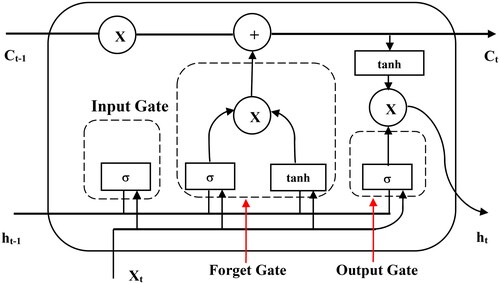
In contrast to conventional FFNNs, the Long Short-Term Memory (LSTM) represents a recurrent neural network design that integrates feedback connections to incorporate information from prior instances into the current one (Dabakoglu, 2019). Its functionality hinges on the backpropagation algorithm, which navigates through the network, layer by layer, from the final to the initial stages. Frequently, standard RNN architectures encounter a hindrance known as the vanishing gradient problem, impeding the effective propagation of valuable gradient information from the model’s initial layers to the current one. To circumvent this obstacle, LSTM units encompass specialised components known as ‘cells’ or ‘memory blocks’ (Abbasimehr et al., 2020).

Figure 1 illustrates the composition of a single LSTM unit, consisting of a cell, an input gate, an output gate and a forget gate. The cell is tasked with preserving the interdependencies among the various elements within an input sequence, while the gates are regulated using sigmoid activation functions. Specifically, the input gate manages the influx of new values into the cell, while the output gate controls the retention of values within the cell. Throughout the training phase, the connections entering and exiting the LSTM gates are assigned weights, a portion of which are recurrent. These weights undergo continuous updates over multiple training cycles (epochs) to enhance the precision of predictions. The incorporation of a forget gate and the additive properties of cell state gradients enable LSTM to adjust connection weights in a manner that significantly mitigates the likelihood of encountering the vanishing gradient problem (Abbasimehr et al., 2020).

Figure 1. Schematic representation of an LSTM RNN Cell.

The predictive capacity of an LSTM RNN is contingent upon the values of two critical tuning parameters: the total number of cells or neurons and the overall number of training cycles or epochs. As a result, it is imperative to compare various LSTM models with distinct neurons and training cycles based on their predictive accuracy using metrics, such as RMSE or MAPE before finalising the LSTM RNN architecture.

Facebook prophet model

Fb Prophet stands as a Bayesian curve fitting-based additive time series model, offering the flexibility to capture intricate time series attributes by incorporating trends and multiple seasonalities, including yearly, monthly, weekly and daily patterns, along with the influence of holidays (Taylor & Letham, 2017). The model’s core components encompass trend g(t), seasonality s(t), holidays h(t) and an error term e(t), as depicted in Equation (12)(12) $$y\left(t\right)=g\left(t\right)+s\left(t\right)+h\left(t\right)+e\left(t\right)$$(12) , where y(t) represents the output value. (12) $$y\left(t\right)=g\left(t\right)+s\left(t\right)+h\left(t\right)+e\left(t\right)$$(12) (13) $$g\left(t\right)=\left(k+a{\left(t\right)}^T\delta \right)t+\left(m+a{\left(t\right)}^T\gamma \right)$$(13)

The trend component, represented by a piecewise linear growth model in Equation (13)(13) $$g\left(t\right)=\left(k+a{\left(t\right)}^T\delta \right)t+\left(m+a{\left(t\right)}^T\gamma \right)$$(13) , involves parameters, such as growth rate (k), time steps (t), adjustment rate (δ), offset parameter (m) and trend change points (γ), allowing for adaptable trend modifications, and was set equal to − s_jδ_j, with a(t) defined in the Equation (14)(14) $$a_j\left(t\right)=\left\{\begin{array}{c}1,t\ge s_j,\\ 0,\mathit{\text{otherwise}}\end{array}\right.$$(14) as: (14) $$a_j\left(t\right)=\left\{\begin{array}{c}1,t\ge s_j,\\ 0,\mathit{\text{otherwise}}\end{array}\right.$$(14)

Additionally, the seasonal component (s(t)) was characterised by a Fourier series model (Equation (15)(15) $$s\left(t\right)=\sum _{n=1}^N\left(a_n\hspace{0.17em}\mathrm{\text{cos}}\hspace{0.17em}\left(\frac{2\pi \mathit{\text{nt}}}{P}\right)+b_n\hspace{0.17em}\mathrm{\text{sin}}\hspace{0.17em}\left(\frac{2\pi \mathit{\text{nt}}}{P}\right)\right)$$(15) ), utilising parameters β to capture cyclic changes based on the periodicity (P) of the data. (15) $$s\left(t\right)=\sum _{n=1}^N\left(a_n\hspace{0.17em}\mathrm{\text{cos}}\hspace{0.17em}\left(\frac{2\pi \mathit{\text{nt}}}{P}\right)+b_n\hspace{0.17em}\mathrm{\text{sin}}\hspace{0.17em}\left(\frac{2\pi \mathit{\text{nt}}}{P}\right)\right)$$(15) where P = 354.25 for yearly seasonality or P = 7 for weekly seasonality. Fitting seasonality term s(t) requires estimating the 2 N parameters β = [a1, b1 ……a_N b_N ]^T.

Moreover, the estimation of the holiday component h(t) relied on an indicator function to determine the presence of holiday events ‘i’ and their corresponding parameter adjustments k_i within the forecast. Notably, Fb Prophet demonstrated resilience in handling outliers and missing data, as well as flexibility in adjusting trends based on events within the time series.

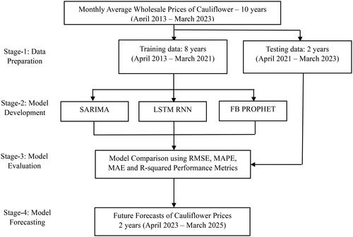
The research methodology, as illustrated in Figure 2, consisted of four stages, beginning with the partitioning of monthly average wholesale prices data of cauliflower into training and testing sets (80–20 ratio). The subsequent model development phase entailed the construction of SARIMA, LSTM RNN and Fb Prophet models using Python and various libraries, such as numpy, pandas, statsmodels, pmdarima and torch (Facebook, 2023; Oliphant, 2006). The ‘pmdarima’ library aided in selecting optimal SARIMA model parameters based on the smallest Akaike Information Criterion (AIC) scores. Likewise, for LSTM RNN models, a range of configurations was tested, with the number of cells and training cycles varied. The models yielding the smallest RMSE and MAPE values were selected for prediction. The Fb Prophet model was executed utilising the open source ‘fbprophet’ library within the Python environment (Facebook, 2023).

Figure 2. Research methodology of the study.

Results and discussions

Model identification and development

The initial step in our data analysis involved a comprehensive visual examination of the historical data through a time series plot, as depicted in Figure 3(a). This examination unveiled a notable clustering of data points around a consistent mean price of Rs. 48.85 per kg. Despite this apparent stability, there were observable variations, with a standard deviation of NRs. Of 23.14 per kg and a range spanning from a minimum price of Rs. 15.95 to a maximum of Rs. 114.21 per kg in consecutive years.

Figure 3. a) Time-series plot of prices of cauliflower (April 2013 to March 2023); b) Seasonal, trend and residual decomposition of time-series data.

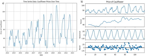
To ascertain the presence of any underlying trends or unit roots within the data, we conducted the ADF test. The results presented in Table 2 revealed that the null hypothesis of the ADF test (H₀: Prices of cauliflower possess a unit root) initially could not be rejected. This prompted us to explore further. Notably, the presence of pronounced yearly seasonal components, as illustrated in Figure 3(b), signaled the need for seasonal differencing. The significance of the p values obtained from the ADF test was notable, revealing respective values of 0.6247 and 0.006 before and after the implementation of seasonal differencing.

Table 2. Unit root test for prices of cauliflower.

ADF Test	Test statistic	Critical value (5%)	p Value	Significance level	Remarks
Before seasonal differencing	−1.309568	−2.888954	0.624784	0.05	Accept H0 (series non-stationary)
After seasonal differencing	−4.217568	−2.892480	0.000615	0.05	Reject H0 (series stationary)

After the examination of the ACF and PACF plots (refer to Figure 4), it was determined that a model characterised by q = 1, Q = 1 or 2, p = 1 or 2 and P = 2 aligned with our stochastic modeling approach. However, subsequent analysis revealed the statistical insignificance of these initial models, as indicated in Table 3. Consequently, a thorough assessment of five alternative models was done with evaluation based on key performance metrics, including the AIC, Bayesian Information Criterion (BIC), R-squared, RMSE and MAPE. Eventually, the SARIMA (0,0,1) (3,1,0)₁₂ model emerged as the most fitting choice. Notably, this model exhibited statistically significant regressors and demonstrated the lowest values across critical performance indicators, including AIC, BIC, RMSE and MAPE.

Figure 4. ACF and PACF plots of seasonally differenced data.

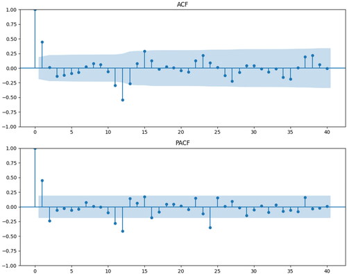
Table 3. Model estimation with AIC, BIC, RMSE and MAPE criterion for SARIMA (p, 0, q) (P, 1, Q)₁₂.

SARIMA model	Akaike information criterion (AIC)	Bayesian information criterion (SBC)	R-Squared	RMSE	MAPE	Remarks
(1,0,1) (2,1,1)12	852.0677	867.4538	0.252694	18.205972	121.187292	SMA (12): 0.978 > 0.05, AR (1): 0.543 > 0.05, MA (1): 0.106 > 0.05
(1,0,1) (2,1,0)12	877.9378	890.7596	0.020949	20.838961	127.936046	AR (1): 0.857 > 0.05
(0,0,1) (2,1,0)12	875.973	886.2305	0.020242	20.846500	127.661862	All regressors significant
(0,0,1) (3,1,0)12	855.4423	868.2641	0.228847	18.494553	133.348233	All regressors significant
(0,0,1) (4,1,0)12	853.476454	868.8623	0.256740	18.156537	130.667024	SAR (48): 0.091 > 0.05

Based on the results of parameter estimators (refer to Table 4), the equation for the SARIMA (0,0,1) (3,1,0)₁₂ with its corresponding coefficients is as follows: (16) $$y_t=1.6693+0.5124{\epsilon }_{t-1}-1.3043y_{t-12}-1.0712y_{t-24}-0.551y_{t-36}+{\epsilon }_t$$(16)

Table 4. Parameter estimators of SARIMA (0, 0, 1) (3, 1, 0)₁₂.

Variable	Coefficient	Std. error	t-Statistic	p Value^a
C	Exp (0.51241) = 1.6693	0.0995	5.1497	***
MA (1)	0.5124	0.100	5.150	***
SAR (12)	−1.3043	0.087	−14.494	***
SAR (24)	−1.0712	0.115	−9.349	***
SAR (36)	−0.5510	0.085	−6.452	***
SIGMASQ	292.4564	46.473	6.293	***

^aLess than 0.05 (*), less than 0.005 (**) and less than 0.0005 (***).

where SIGMASQ term represents the variance of the error term (ε_t) in the model.

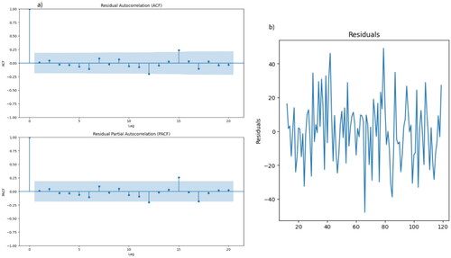
The Ljung-Box Q statistic, with a value of 0.11 and a corresponding probability of 0.74, indicates the absence of significant autocorrelation in the residuals, suggesting a good fit of the model. Similarly, the Jarque-Bera statistic, yielding a low value of 0.44 and a high probability of 0.80, supports the approximation of normality within the dataset. The assessment for heteroskedasticity reveals a value of 1.50, alongside a two-sided probability of 0.26, suggesting the absence of significant heteroskedasticity in the data. Furthermore, the skewness value of −0.09 indicates a slight left skew in the data distribution, while the kurtosis value of 3.27 signifies a moderately peaked distribution. Collectively, these diagnostics validate the SARIMA model’s robustness and its adherence to key statistical assumptions, reinforcing its credibility in accurately capturing and forecasting the underlying time series dynamics.

In addition to the diagnostic measures mentioned above, the analysis of the SARIMA model extends to the examination of residual autocorrelation and partial autocorrelation functions (ACF and PACF). Figure 5(a) showcases the residual ACF and PACF plots, demonstrating the absence of significant autocorrelation in the residuals, further reinforcing the model’s adequacy. Moreover, the residuals presented in Figure 5(b) conform to the characteristics of white noise.

Figure 5. a) Residual ACF and PACF plots of SARIMA (0 0, 1) (3, 1, 0)12; b) residual time-series plot.

Considering this observation, a shift towards an alternate modeling approach was considered, leading to the exploration of the LSTM RNN as a potential candidate for enhanced predictive capabilities. Specifically, a systematic investigation was conducted, varying the number of neurons and epochs, with a focus on minimising both the RMSE and the MAPE. Among the five alternative models assessed (refer to Table 5), the LSTM RNN model configured with 100 neurons and trained over 50 epochs demonstrated the most promising performance characteristics. Notably, this configuration effectively balanced computational efficiency with heightened predictive accuracy, allowing for the capture of intricate temporal dependencies and the recognition of complex patterns inherent within the dataset.

Table 5. Number of neurons and Epochs considered in five LSTM RNN models.

Model	No. of neurons	No. of Epochs	RMSE	MAPE
LSTM1	100	50	31.803930	42.945598
LSTM2	100	60	45.500532	90.419521
LSTM3	100	40	33.462227	61.681581
LSTM4	150	50	40.360049	78.319300
LSTM5	150	40	48.156613	104.973604

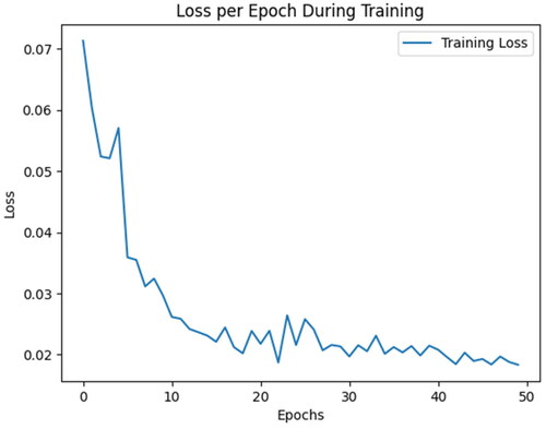
The graphical representation in Figure 6 illustrates the loss per epoch plot, showcasing a notable trend in the model’s performance during the training phase. The plot demonstrates an initial sharp decline in the loss value over the first 10 epochs, indicative of rapid improvements in the model’s convergence. Subsequently, the plot exhibits fluctuations in the loss value up to 30 epochs, suggesting the model’s gradual fine-tuning process and sensitivity to training dynamics. Notably, beyond the 40th epoch, the loss value stabilises, approaching an asymptotic pattern, signifying a relatively steady state of model optimisation. This visualisation offers valuable insights into the dynamics of the model’s learning process and its convergence trajectory, highlighting key phases of rapid improvement, gradual refinement, and eventual stabilisation.

Figure 6. Loss per Epoch during training of LSTM₁ model.

Model comparision

Notably, within the in-sample analysis (refer to Table 6), the SARIMA model demonstrates an R-squared value of 0.3339, indicating a relatively adequate fit, while the LSTM RNN model exhibits a lower R-squared value of −0.1261. In contrast, the Fb Prophet model stands out with a significantly higher R-squared value of 0.6592, clearly surpassing the SARIMA model by a substantial margin. This significant disparity underscores the Fb Prophet model’s exceptional capability in elucidating the variance within the training dataset, emphasising its superior fit and proficiency in capturing the underlying data patterns.

Table 6. Comparison of in-sample and out-sample performances of SARIMA, LSTM RNN and Fb Prophet models.

	Performance metrics	SARIMA forecast	LSTM RNN forecast	Fb Prophet forecast
In-sample (training)	R-squared	0.3339	−0.1261	0.6592
	MAE	15.3870	24.0741	10.5941
	RMSE	20.4719	31.8039	13.4144
	MAPE	36.6410	42.9456	27.5700
Out-sample (testing)	R-squared	0.6434	0.0525	0.5744
	MAE	10.5913	15.6799	11.4158
	RMSE	13.0242	21.2287	14.2280
	MAPE	21.4064	39.1171	23.6645

Conversely, the out-sample metrics, which reflect the models’ predictive performance on unseen data, indicate a notable shift in the results. While the SARIMA model continues to maintain a relatively high R-squared value of 0.6434, suggesting its capability to explain the variance in the data, the LSTM RNN model (0.0525) and the Fb Prophet model (0.5744) exhibit comparatively lower performance. Similarly, the SARIMA model demonstrates lower values for metrics, such as MAE, RMSE and MAPE in the out-sample evaluation, signifying its relatively superior predictive accuracy on unseen data compared to the LSTM RNN and Fb Prophet models.

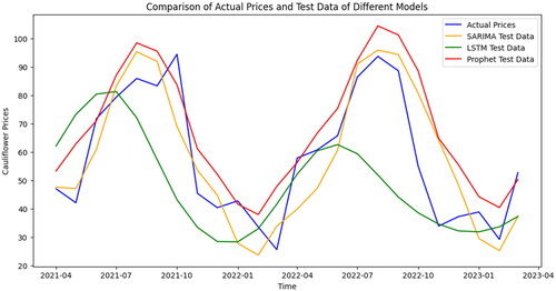
Figure 7 provides a visual representation of the model’s predictive performance, contrasting the actual values with the predictions on testing data spanning from 1 April 2021 to 1 March 2023. This timeframe aligns with the established 80 − 20 training-testing data split and offers a comprehensive view of how well the model’s forecasts correspond with the real values during this evaluation period.

Figure 7. Comparison of actual vs. predicted test data of different models.

Future forecasts of cauliflower prices

While the Fb Prophet model demonstrated commendable accuracy during the in-sample training phase, the intriguing finding was the pronounced advantage of a parsimonious non-linear statistical model like SARIMA when forecasting unseen (out-sample) data. This revelation underscores the need for a carefully considered choice of modeling approach in different scenarios. With this insight, the subsequent 24-month future forecasts for cauliflower prices were meticulously conducted using the SARIMA (0,0,1) (3,1,0)₁₂ model, which proved to be a robust and reliable choice for extrapolating trends and patterns into the future. This strategic selection was driven by the model’s remarkable performance in capturing both the seasonal and non-seasonal components of the data, particularly when faced with previously unseen data.

To facilitate a comprehensive evaluation and enable an informed decision regarding the most suitable forecasting strategy for future periods, the forecasts generated by the LSTM and Fb Prophet models have also been included. These results, presented in Figure 8 and Table 7, serve as valuable reference points for a comparative analysis of the predictive capabilities of the various modeling approaches.

Figure 8. a) Forecasts using SARIMA model, b) Forecasts using Fb Prophet model and c) Forecasts using LSTM RNN model.

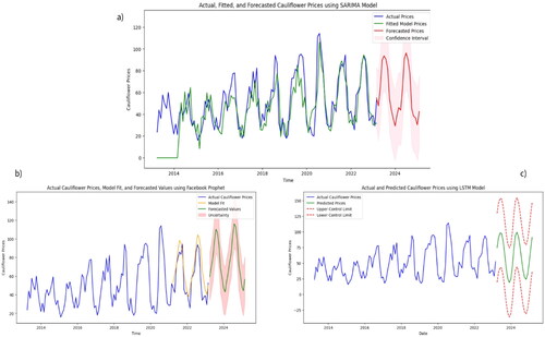
Table 7. Future forecasts of cauliflower prices using different models.

Date	SARIMA forecasts	Fb Prophet forecasts	LSTM RNN forecasts	Date	SARIMA forecasts	Fb Prophet forecasts	LSTM RNN forecasts
April, 2023	54.852	59.402	61.189	April, 2024	46.126	63.460	51.036
May, 2023	47.740	70.323	70.778	May, 2024	43.712	74.598	56.999
June, 2023	64.186	79.737	77.485	June, 2024	62.650	83.952	58.345
July, 2023	89.759	97.678	78.577	July, 2024	90.987	102.802	55.319
August, 2023	93.591	110.415	70.772	August, 2024	96.270	116.240	49.086
September, 2023	90.741	106.965	57.378	September, 2024	89.908	112.755	42.383
October, 2023	81.796	93.475	44.773	October, 2024	77.431	98.791	37.687
November, 2023	54.032	68.624	36.038	November, 2024	45.016	71.944	34.656
December, 2023	43.692	58.899	31.124	December, 2024	38.171	61.252	33.381
January, 2024	35.951	46.890	30.886	January, 2025	36.915	48.922	33.868
February, 2024	29.232	42.992	35.080	February, 2025	30.302	44.409	35.965
March, 2024	39.481	54.280	42.587	March, 2025	41.624	56.721	39.192

All three models have proven their efficacy in capturing the underlying trends in cauliflower price data, demonstrating a remarkable alignment of their forecasted series with the actual series during the specified period. To gauge accuracy, we relied on both the RMSE and MAPE. The computed RMSE values were NRs – 13/kg, NRs – 21/kg and NRs – 14/kg for the SARIMA, LSTM RNN and Fb Prophet models, respectively, further elucidating the degree of deviation between the forecasted and actual values. In terms of MAPE, the values were approximately 21%, 39% and 24% for the SARIMA, LSTM RNN and Fb Prophet models, respectively, reflecting the extent of forecast deviation. Notably, the SARIMA model exhibited the lowest RMSE and MAPE values, indicating its superior precision in forecasting, followed by the Fb Prophet model and the LSTM RNN model.

Considering the potential influence of various external factors on cauliflower prices, including climate conditions, pest infestations, the effects of recent pandemics like COVID-19 and the reliance on imports during festival seasons (September–November), the forecast accuracies attained are deemed acceptable. Additionally, market dynamics, trade policies and export conditions can contribute to unpredictable price fluctuations. The forecasted prices demonstrate a stationary structure, indicating that significant price changes are not expected under normal conditions until the first quarter of 2025.

Discussion

The findings of this study, within the context of Nepal’s cauliflower market, corroborate the significant contributions of established literature while also providing fresh perspectives on the suitability of various forecasting methods. Notably, the outperformance of SARIMA over more complex models like LSTM RNN and Fb Prophet in predicting cauliflower prices might be somewhat unexpected given the trend towards machine learning in recent research. However, it aligns with earlier observations by Geweke and Porter-Hudak (1983) and Luo et al. (2013), highlighting the enduring importance of seasonality in agricultural time series data.

Upon deeper analysis, the superior performance of SARIMA in our study suggests that the conceptual simplicity of statistical models, in certain circumstances, becomes their strength. In markets like Nepal where data may be noisy or sparse, the parsimony of SARIMA avoids the overfitting challenges sometimes faced by its machine-learning counterparts, a sentiment echoed in the skepticism of Zhang et al. (2018) and Abbasimehr et al. (2020) towards applying advanced models without sufficient consideration for context.

Our study contributes to the ongoing conversation about the importance of model selection in empirical research, reinforcing the idea that the most effective model is not always the most complex one. In applying these insights to the cauliflower market in Nepal, we highlight the need for data-driven, nuanced approaches to agricultural forecasting – a recommendation that speaks directly to the calls for methodological diversity by Majhi et al. (2023) and others advocating for hybrid modeling techniques.

Conclusion and policy implications

Our in-depth investigation of cauliflower pricing dynamics within Nepal, employing the analytical power of Google Colab and Python’s vast array of libraries, has provided a granular view of the forces at play within this sector of the agricultural market. We have determined a pronounced seasonal influence on pricing without any significant long-term price trends, as unambiguously delineated by the seasonal adjustment capabilities of the SARIMA model in our time series analysis. Despite exploring more complex, non-linear alternatives like the LSTM and Fb Prophet models, it was the SARIMA model that most accurately predicted price fluctuations – a result that defies previous evidence from fields as divergent as utilities and public health, where intricate models generally prevailed.

This outcome underscores the indispensability of a context-specific approach in predictive modeling, pointing towards the necessity of calibrating methodologies to the peculiarities inherent in the subject data. It also brings forth an appreciation for the predictably steady price outlook for cauliflower up to the first quarter of 2025, as foreseen by the SARIMA (0,0,1) (3,1,0)₁₂ model, although this stability in pricing is not devoid of its challenges. With constant prices comes the potential pressure of rising production costs, a situation that if unaddressed, could culminate in diminished returns for cauliflower growers.

Considering the patterns identified in our forecasting analysis, the strategic shift towards off-season cauliflower production offers a compelling avenue for local farmers to leverage consistent pricing to their advantage. This recommendation gains relevance in light of the seasonal demand spikes during festival seasons – primarily from September to November – wherein price surges concurrently elevate import volumes to meet domestic needs.

As part of a broader policy framework, we propose the following targeted interventions to enable this strategic pivot:

1. Financial incentive programs: Establish financial incentive programs aimed at reducing the economic barriers to off-season farming. These could take the form of interest-free loans, grants or subsidies for seeds, fertilisers, and necessary equipment that aid farmers in capitalising on favorable market conditions.

2. Information dissemination and education: Enhance the dissemination of actionable agricultural data to farmers through mobile technology platforms and community-based educational programs. By increasing farmers’ understanding of market cycles and the benefits of off-season production, these initiatives can optimise decision-making and crop planning.

3. Infrastructure development: Accelerate investment in essential infrastructure, such as cold storage facilities and efficient transportation networks. These developments ensure harvested crops can be preserved for longer periods, thereby mitigating spoilage and facilitating sale during peak price periods.

4. Stabilisation policies: Implement stabilisation policies, such as price supports or guaranteed purchase agreements for off-season produce. Such measures could protect farmers from unexpected dips in market prices, ensuring consistent revenue streams.

5. Risk management schemes: Introduce crop insurance and risk management schemes tailored specifically for off-season production risks, providing a safety net for farmers against adverse weather events or unexpected market shifts.

6. Market expansion initiatives: Support market expansion efforts, enabling farmers to access new and more lucrative markets, potentially across borders. This could involve trade agreements and partnerships that prioritise agricultural exports.

7. Sustainability and resource management: Promote sustainable practices and efficient resource management to maintain soil health and fertility, especially important with potentially increased cultivation frequencies involved in offseason production.

By promoting these measures, the larger goal seeks to catalyse a resilient, self-reliant agricultural sector within Nepal. These policy prescriptions are designed not merely to navigate the present market landscape but to propel the sector towards a future where it can weather economic fluctuations, reduce import-dependency, and promote sustainability. It is through such a comprehensive and responsive policy ecosystem that Nepal can secure the foundations of its agricultural economy and uphold the livelihoods of its farming communities.

Author’s contributions

Anisha Giri: Conceived and designed the study, performed data collection and compilation from secondary sources, conducted analysis and conducted relevant literature review.

Vijay Raj Giri: Contributed to documenting the research process, prepared the manuscript, compiled reports and meticulously verified the analysis conducted by the main author.

Acknowledgements

The authors have no acknowledgments to make.

Availability of supporting data

All data generated or analysed during this study are included in this article and its Supplementary Information files.

Disclosure statement

The authors declare that they have no competing interests.

Additional information

Funding

The research reported in this article received no specific funding.

Notes on contributors

Anisha Giri

Anisha Giri is an Agrieconomist at the Government of Nepal, working under the Ministry of Agriculture and Livestock Development. She holds a Master’s degree in Agronomy from the Agriculture & Forestry University (AFU), Nepal, as well as a Master’s in Public Administration (MPA) and a Bachelor’s of Science (BSc) degree in Agriculture from Tribhuvan University (T U), Nepal. With seven years of dedicated service, Anisha is now seeking to explore and integrate machine learning and AI techniques in her study. Her other research interests include agribusiness management, consumer behaviour, econometrics, and statistical analysis.

Vijay Raj Giri

Vijay Raj Giri is a doctoral candidate in Mechanical Sciences and Engineering at the University of Michigan-Dearborn and a Graduate Student Research Assistant. He holds an MSc in Renewable Energy Engineering and a Bachelor’s in Mechanical Engineering from the Pulchowk Campus, Institute of Engineering, Tribhuvan University, along with an MPA from T U. His research focuses on combustion, SI engine modeling, knocking phenomena, phenomenological models, and the application of machine learning in these areas.

References

- Abbasimehr, H., Shabani, M., & Yousefi, M. (2020). An optimized model using LSTM network for demand forecasting. Computers and Industrial Engineering. 143, 1. https://doi.org/10.1016/j.cie.2020.106435
- Yercan, M., & Adanacioglu, H. (2012). An analysis of tomato pricesat wholesale level in Turkey: an application of SARIMA model. Custos e Agronegocio, 8, 52–75. Retrieved from: http://www.custoseagronegocioonline.com.br/numero4v8/Tomato%20english.pdf
- Adebiyi, A. A., Adewumi, A. O., & Ayo, C. K. (2014). Stock price prediction using the ARIMA model. Journal of Emerging Trends in Computing and Information Sciences, 5(4), 295–17. https://doi.org/10.1109/UKSim.2014.67
- AEC. (2006). Off-season vegetables. Agro Enterprise Center/FNCCI.
- Alibuhtto, M. C., & Ariyarathna, H. R. (2019). Forecasting weekly temperature using the ARIMA model: a case study for Trincomalee in Sri Lanka. Int J Sci Environ Technol, 8(1), 124–131. https://www.semanticscholar.org/paper/FORECASTING-WEEKLY-TEMPERATURE-USING-ARIMA-MODEL-%3A-Alibuhtto-Ariyarathna/57f5644aead014f77b878ef31b64dbc1208c6c96#citing-papers
- Arunraj, N. S., Ahrens, D., & Fernandes, M. (2016). Application of SARIMAX model to forecast daily sales in the food retail industry. International Journal of Operations Research and Information Systems, 7(2), 1–21. https://doi.org/10.4018/IJORIS.2016040101
- Bisht, M., & Kumar, R. (2019). Estimating volatility in prices of pulses in India: An application of GARCH model. Economic Affairs, 64(3), 513–516. https://doi.org/10.30954/0424-2513.3.2019.6
- Box, G. E., Jenkins, G. M., Reinsel, G. C., & Ljung, G. M. (2015). Time series analysis: Forecasting and control. John Wiley & Sons. https://doi.org/10.1111/jtsa.12194
- CASA. (2020). Vegetable sector strategy - Nepal. Commercial Agriculture for Smallholders and Agribusiness (CASA) Nepal Country Team. Retrieved October 20, 2023, from https://www.casaprogramme.com/wp-content/uploads/CASA-Nepal-VegetablesSector-analysis-report.pdf
- Chatfield, C. (2016). Analysis of time series: An introduction. CRC Press. https://doi.org/10.4324/9780203491683
- Chen, K. Y., & Wang, C. H. (2007). A hybrid SARIMA and support vector machines in forecasting the production values of the machinery industry in Taiwan. Expert Systems with Applications, 32(1), 254–264. https://doi.org/10.1016/j.eswa.2005.11.027
- Choudhury, A., & Jones, J. (2014). Crop yield prediction using time series models. Journal of Economics and Economic Education Research, 15(3), 53–67. Retrieved from https://www.researchgate.net/publication/288387590_Crop_yield_prediction_using_time_series_models
- Christensen, C., Wagner, T., & Langhals, B. (2021). Year-independent prediction of food insecurity using classical and neural network machine learning methods. AI, 2(2), 244–260. https://doi.org/10.3390/ai2020015
- da Veiga, C. P., da Veiga, C. P., Catapan, A., Tortato, U., & Silva, W. V. (2014). Demand forecasting in food retail: A comparison between the Holt-Winters and ARIMA models. WSEAS Transactions on Business and Economics, 11(1), 608–614. https://www.researchgate.net/publication/286314562_Demand_forecasting_in_food_retail_A_comparison_between_the_Holt-Winters_and_ARIMA_models
- Dabakoglu, C. (2019, June 23). Time series forecasting - ARIMA, LSTM, Prophet with Python. Medium.com. https://medium.com/@cdabakoglu/time-series-forecasting-arima-lstm-prophet-with-python-e73a750a9887
- Deléglise, H., Interdonato, R., Bégué, A., d’Hôtel, E. M., Teisseire, M., & Roche, M. (2022). Food security prediction from heterogenous data combining machine and deep learning methods. Expert Systems with Applications, 190, 116189. https://doi.org/10.1016/j.eswa.2021.116189
- Divisekara, R., Jayasinghe, G., & Kumari, K. (2021). Forecasting the red lentils commodity market price using SARIMA models. SN Business & Economics, 1(1). https://doi.org/10.1007/s43546-020-00020-x
- Esther, W., & Magdaline, K. (2017). Forecasting pulses production in Kenya using ARIMA model. Asian Journal of Economics, Business and Accounting, 2(3), 1–8. https://doi.org/10.9734/AJEBA/2017/32414
- Facebook. (2023). Quick start prophet. Retrieved October 20, 2023, from GitHub: https://github.com/facebook/prophet
- Geweke, J., & Porter-Hudak, S. (1983). The estimation and application of long memory time series models. Journal of Time Series Analysis, 4(4), 221–238. https://doi.org/10.1111/j.1467-9892.1983.tb00371.x
- Ghimire, D., Lamsal, G., Paudel, B., Khatri, S., & Bhusal, B. (2018). Analysis of trend in area, production, and yield of major vegetables of Nepal. Trends in Horticulture, 1(2), 1–11. https://doi.org/10.24294/th.v1i2.914
- Giri, A., & Giri, V. R. (2023). Comparative assessment of SARIMA and SSES models for forecasting cucumber prices in Nepal. Advances in Applied Sciences, 8(3), 106–121. https://doi.org/10.11648/j.aas.20230803.17
- Guo, Y., Tang, D., Tang, W., Yang, S., Tang, Q., Feng, Y., & Zhang, F. (2022). Agricultural price prediction based on combined forecasting model under spatial-temporal influencing factors. Sustainability, 14(17), 10483. https://doi.org/10.3390/su141710483
- Hamzacebi, C. (2008). Improving artificial neural networks’ performance in seasonal time series forecasting. Information Sciences, 178(23), 4550–4559. https://doi.org/10.1016/j.ins.2008.07.024
- Hernandez-Matamoros, A., Fujita, H., Hayashi, T., & Perez-Meana, H. (2020). Forecasting of COVID-19 per regions using ARIMA models and polynomial functions. Applied Soft Computing, 96, 106610. https://doi.org/10.1016/j.asoc.2020.106610
- Kamruzzaman, J., Sarker, R. A., & Hossain, M. A. (2006 Forecasting of daily rainfall using artificial neural network: A case study on Bangladesh [Paper presentation]. International Conference on Computer and Communication Engineering. Kuala Lumpur, Malaysia.
- Kaur, H., & Ahuja, S. (2019). SARIMA modelling for forecasting the electricity consumption of a health care building. International Journal of Innovative Technology and Exploring Engineering (IJITEE), 8(12), 2795–2799. https://www.ijitee.org/wp-content/uploads/papers/v8i12/L25751081219.pdf
- Kihoro, J. M., Otieno, R.O., & Wafula, C.(2004). Seasonal time series forecasting: A comparative study of ARIMA and ANN models. African Journal of Science and Technology (AJST), Science and Engineering Series, 5(2), 41-49. Retrieved from https://citeseerx.ist.psu.edu/document?repid=rep1&type=pdf&doi=123af7e5b9dd2171826ca4f3df50406d9df4459a
- Le, T., Vo, B., Fujita, H., Nguyen, N. T., & Baik, S. W. (2019). A fast and accurate approach for bankruptcy forecasting using squared logistics loss with GPU-based extreme gradient boosting. Information Sciences, 494, 294–310. https://doi.org/10.1016/j.ins.2019.04.060
- Luo, C. S., Zhou, L. Y., & Wei, Q. F. (2013). Application of SARIMA Model in Cucumber Price Forecast. Applied Mechanics and Materials, 373–375, 1686–1690. https://doi.org/10.4028/www.scientific.net/amm.373-375.1686
- Majhi, S. K., Bano, R., Srichandan, S. K., Acharya, B., Al-Rasheed, A., Alqahtani, M. S., & Soufiene, B. O. (2023). Food price index prediction using time series models: A study of Cereals, Millets and Pulses. Research Square, https://doi.org/10.21203/rs.3.rs-2999898/v1
- MoALD. (2020). Vegetable production in Nepal: Constraints and challenges. Ministry of Agriculture and Livestock Development (MoALD), Government of Nepal (GoN).
- MoALD. (2023). Statistical information on Nepalese agriculture FY 2021/22. Ministry of Agriculture and Livestock Development, Government of Nepal.
- Mutwiri, M., Gichuhi, R., & Wabwoba, F. (2019). Forecasting of tomatoes wholesale prices of Nairobi in Kenya: Time series analysis using SARIMA model. International Journal of Statistical Distributions and Applications, 5(3), 46–53. https://doi.org/10.11648/j.ijsd.20190503.11
- Department of Customs, Government of Nepal (2023). Nepal foregn trade statistics. Department of Customs, Government of Nepal.
- Oliphant, T. E. (2006). Guide to NumPy. https://ecs.wgtn.ac.nz/foswiki/pub/Support/ManualPagesAndDocumentation/numpybook.pdf
- Oswari, T., Yusnitasari, T., Kusumawati, R., & Setiawan, I. (2022). Prediction analysis of food crop farmer index price during Covid-19 pandemic using ARIMA and LSTM. Journal of Management Information and Decision Sciences, 25(2S), 1–10. https://www.abacademies.org/articles/prediction-analysis-of-food-crop-farmer-index-price-during-covid19-pandemic-using-arima-and-lstm-13360.html
- Otu, A. A., Osuji, G. A., Opara, J., Mbachu, H. I., & Iheagwara, A. I. (2014). Application of Sarima models in modelling and forecasting Nigeria’s inflation rates. American Journal of Applied Mathematics and Statistics, 2(1), 16-28. https://doi.org/10.12691/ajams-2-1-4
- Ouyang, H., Wei, X., & Wu, Q. (2019). Agricultural commodity futures prices prediction via long- and short-term time series network. Journal of Applied Economics, 22(1), 468–483. https://doi.org/10.1080/15140326.2019.1668664
- Permanasari, A. E., Hidayah, I., & Bustoni, I. A. (2013). SARIMA (Seasonal ARIMA) implementation on time series to forecast the number of Malaria incidence [Paper presentation]. Proceedings of 2013 International Conference on Information, Technology and Electrical Engineering (ICITEE)., Yogyakarta, Indonesia. https://doi.org/10.1109/ICITEED.2013.6676239
- Petruzzello, M. (2024). Cauliflower. Encyclopedia Britannica, 2 Feb. 2024, https://www.britannica.com/plant/cauliflower.
- Poudel, R. (2019). Understanding cauliflower production in Changunarayan municipality: A case study. Journal of Horticultural Sciences, 6(4), 123–137.
- Purohit, S. K., Panigrahi, S., Sethy, P. K., & Behera, S. K. (2021). Time series forecasting of price of agricultural products using hybrid methods. Applied Artificial Intelligence, 35(15), 1388–1406. https://doi.org/10.1080/08839514.2021.1981659
- Rahman, N., Jia, G., & Zulkafli, H. (2023). GARCH models and distributions comparison for nonlinear time series with volatilities. Malaysian Journal of Fundamental and Applied Sciences, 19, 989–1001. https://doi.org/10.11113/mjfas.v19n6.3101
- Rajeswari, S., & Suthendran, K. (2019). Developing an agricultural product price prediction model using HADT algorithm. International Journal of Engineering and Advanced Technology, 9(1S4), 569–575. https://doi.org/10.35940/ijeat.A1126.1291S419
- Rohith, R., Vishnu, R., Kishore, A., & Chakkarawarthi, D. (2020). Crop price prediction and forecasting system using supervised machine learning algorithms. International Journal of Advanced Research in Computer and Communication Engineering (IJARCCE), 9(3), 27–29. https://doi.org/10.17148/IJARCCE.2020.9306
- Sarangi, P. K., Sinha, D., Sinha, S., & Mittal, N. (2021). Machine Learning Approach for the Prediction of Consumer Food Price Index. Proceedings of [Paper presentation]. 2021 9th International Conference on Reliability, Infocom Technologies and Optimization (Trends and Future Directions) (ICRITO). Noida, India. https://doi.org/10.1109/ICRITO51393.2021.9596527
- Sellam, V., & Poovammal, E. (2016). Prediction of crop yield using regression analysis. Indian Journal of Science and Technology, 9(38), 1–5. https://doi.org/10.17485/ijst/2016/v9i38/91714
- Selvanayagam, T., Suganya, S., Palendrarajah, P., Manogarathash, M. P., Gamage, A., & Kasthurirathna, D. (2019). Agro-genius: Crop prediction using machine learning. International Journal of Innovative Science and Research Technology, 4(10), 243–249. https://ijisrt.com/assets/upload/files/IJISRT19OCT1880.pdf
- Shet, A., S., A., Naik, D., Shetty, S., & K., R. (2022). Stock price prediction using machine learning. International Journal of Engineering Applied Sciences and Technology, 7, 225-228. https://doi.org/10.33564/IJEAST.2022.v07i02.034
- Shumway, R. H., & Stoffer, D. S. (2017). Time series analysis and its applications: With R examples. Springer.
- Souza, R. C. T. de, Guedes Filho, O., Santos, M. A. R. dos, & Coelho, L. dos S. (2016). Monthly closing price forecasting of soybean grain in Paraná using SARIMA modeling with intervention. Journal of Geospatial Modeling, 2(1), 27–44. https://doi.org/10.22615/2526-1746-jgm-2.1-5887
- Taylor, S. J., & Letham, B. (2017). Forecasting at scale. PeerJ Preprints, 35(8), 48–90. https://doi.org/10.7287/peerj.preprints.3190v2
- Vibas, V. M., & Raqueño, A. R. (2019). A Mathematical Model for Estimating Retail Price Movements of Basic Fruit and Vegetable Commodities Using Time Series Analysis. International Journal of Advance Study and Research Work, 2(7), 01–05. https://doi.org/10.5281/zenodo.3333529
- Wamalwa, T. M., & Muchemi, L. (2020). An artificial neural network model for predicting maize prices in Kenya. Africa Journal of Physical Sciences, 4, 54–59. http://jsep.uonbi.ac.ke/ojs/index.php/ajps/article/view/1016/922
- Wang, Y., Ye, X., & Huo, Y. (2011). Prediction of household food retail prices based on ARIMA Model [Paper presentation]. Proceedings of 2011 International Conference on Multimedia Technology. Hangzhou. https://doi.org/10.1109/ICMT.2011.6002376
- Zahara, S., Sugianto, S. & Ilmiddaviq, M. B. (2019 Consumer price index prediction using Long Short Term Memory (LSTM) based cloud computing [Paper presentation]. The 5th International Conference on Technology and Vocational Teachers (ICTVT 2019), 14–15 September 2019. Yogyakarta, Indonesia. https://doi.org/10.1088/1742-6596/1456/1/012022
- Zhang, D., Zang, G., Li, J., Ma, K., & Liu, H. (2018). Prediction of soybean price in China using QR-RBF neural network model. Computers and Electronics in Agriculture, 154, 10–17. https://doi.org/10.1016/j.compag.2018.08.016