Enhancing irrigation water management based on ETo prediction using machine learning to mitigate climate change

Abstract

This study addressed the increasing challenges of climate change by exploring the use of machine learning (ML) algorithms to predict the reference evapotranspiration (ETo). Accurate ETo prediction is crucial for optimizing irrigation water management. This research aimed to assess the reliability and accuracy of ML algorithms in predicting ETo values. Three ETo calculation methods were employed: Penman-Monteith (PM), Hargreaves (HA), and Blaney-Criddle (BC). The study analyzed ETo and other climate variables using the modified Mann-Kendall test (m-MK) and Theil Sen’s slope estimator methods to identify trends. Multiple ML algorithms, including Support Vector Regression (SVR), Random Forest (RF), XGboost, K-Nearest Neighbor (KNN), Decision Trees (DT), Linear Regression (LR), and Multiple Linear Regression (MLR) were utilized for ETo prediction. The ML algorithms exhibited excellent performance, with coefficients of determination (R²) values ranging from 0.97 to 0.99 for PM, 0.99 for HA, and from 0.91 to 0.92 for BC. The models demonstrated a high value of the Kling-Gupta efficiency (KGE) with low Root Mean Square Error (RMSE) and Mean Absolute Error (MAE) values. Strong correlations between the predicted and calculated daily ETo were observed with R² values of 0.99, 0.99, and 0.92 for PM, HA, and BC methods, respectively. In conclusion, this study affirmed the accuracy and reliability of ML algorithms to match that of standard ETo prediction equations.

Keywords:

• Climate change
• reference evapotranspiration
• machine learning algorithms
• modified Mann-Kendall test
• Kling-Gupta efficiency

REVIEWING EDITOR:

• Manuel Tejada, Universidad de Sevilla, Spain

SUBJECTS:

• Agriculture & Environmental Sciences
• Agriculture and Food
• Agriculture

1. Introduction

Climate change, population growth, and inadequate water management all contribute to the worldwide issue of water resource management (Sharma & Irmak, 2012). Efficient water management requires precise determination of crop irrigation needs and optimal timing and quantity of water application (Allen et al., 1998; Chouaib et al., 2022). Evapotranspiration is the result of soil surface evaporation combined with plant transpiration (Allen et al., 1998). Reference evapotranspiration (ETo) is a crucial parameter in plant water requirements, irrigation scheduling, planning, and management. It represents the rate of evapotranspiration calculated using the characteristics of a reference crop, typically a well-watered grass surface with specific properties such as a crop height of 0.12 m, an albedo of 0.23, and a surface resistance of 70 m/s (Allen et al., 1998). ETo has significant implications for hydrological and agrometeorological processes due to its integral role in these domains (Allen et al., 1998; Sentelhas et al., 2010). Precise determination of ETo is crucial for the efficient planning and management of irrigation strategies (Hu et al., 2022; Nauman et al., 2023). By understanding ETo, farmers and agronomists can make informed decisions about when and how much water to apply to their crops (Kumar et al., 2011; Raza et al., 2020).

Two approaches exist for determining reference evapotranspiration (ETo): direct and indirect methods. Direct methods, such as lysimeter and eddy covariance techniques, rely on water balance and vapor transfer principles. Among these methods, eddy covariance is known for providing highly accurate results (Ndulue & Ranjan, 2021). However, these direct methods can be time-consuming, costly, and require specialized expertise (Allen et al., 1998). On the other hand, indirect methods rely on meteorological data obtained from weather stations. These methods employ empirical or physically based equations that establish relationships between ETo and weather parameters. Indirect methods are typically based on solar radiation fluxes, temperatures, and aerodynamic properties (Kumar et al., 2011).

With its reliable correlation to lysimeter data and ability to generate consistent ETo values in diverse climates and regions, the FAO-PM equation stands out as a recommended choice for predicting ETo (Allen et al., 1998). While the Penman-Monteith (PM) equation is renowned for its precision in calculating ETo, it requires the input of various climatic parameters that may not always be obtainable (dos Santos Farias et al., 2020).

For regions in which local weather stations don’t have access to the complete range of meteorological parameters necessary for utilizing the PM method to estimate ETo, farmers and agronomists must choose alternative ETo estimation techniques (Hafeez et al., 2020; Thongkao et al., 2022).

Given that it requires only air temperature, the Hargreaves (HA) equation is a simple and user-friendly method for determining ETo (Djaman et al., 2019; Hargreaves & Samani, 1985). Research on the effectiveness of the HA equation for estimating ETo (Allen et al., 1998) noted that the equation tends to underestimate ETo in conditions of wind speeds exceeding 3 m/s and overestimate ETo at high relative humidity levels. Aschonitis et al. (2017) conducted a study aimed at improving the global estimation of ETo by recalibrating the annual coefficients for the HA equation. de Sousa Lima et al. (2013) adapted the HA equation to suit the climate of Iran, discovering that changing the constant from 0.0023 to 0.0018 and 0.0037 in semiarid and arid regions, respectively, enhanced the accuracy of the equation.

The FAO proposed the BC method as another temperature based ETo method. Since it relies on temperature alone, the BC equation is another practical alternative to the PM equation in conditions where there is a lack of meteorological data or when it is impossible to perform sophisticated computations (Hafeez et al., 2020; Mobilia & Longobardi, 2021). The agricultural community has accepted the FAO BC method for estimating ETo (Thongkao et al., 2022). Despite its ease of use, it delivers findings that are correct in a wide range of environments and climatic conditions, making it a significant tool for agricultural water management (Heydari et al., 2015).

Given the nonlinear, dynamic, and complex physical processes associated with estimating ET from weather data, creating a formula that accurately handles these processes is a formidable task (Wen et al., 2015). Machine learning (ML) algorithms are now a promising alternative to traditional methods because they can handle complex and nonlinear processes exceptionally well (Ferreira et al., 2019). The efficiency of ML models to handle multidimensional data and perform autonomous decision-making without human intervention is a significant benefit. However, an initial dataset to train the ML system is necessary, with subsequent decisions being based on this training data. Despite its benefits, ML also faces several challenges, including the complexity of the problem, selecting or developing appropriate models, selecting optimal hardware, and verifying model performance and accuracy in real-world situations (Azzam et al., 2022; Meshram et al., 2021).

To ensure that the ML model remains optimized for the most recent data, the model need to be updated with new data and tested using part of the data. The researchers used statistical measures, including the root mean squared error (RMSE) and the coefficient of determination (R²). Researchers acquire a better understanding of the model’s strengths and limitations by employing both metrics, facilitating future development and improvement (Farooque et al., 2022).

Enhancing prediction accuracy and creating trustworthy models are significant ML challenges. Giving the model more training data, using larger architectures, and assigning more computer resources, can help accomplish this (Ravindran et al., 2021). ML algorithms have demonstrated their potential for precise estimation of both reference and actual evapotranspiration in various climatic conditions. To predict ETo using ML algorithms, relevant methodologies have been informed by recent studies conducted by (Bashir et al., 2023; Chen et al., 2020; Granata, 2019; Kar et al., 2021; Khan et al., 2022; Tausif et al., 2023). Additionally (Granata & Di Nunno, 2021; White et al., 2008), used ML algorithms to accurately estimate and anticipate actual evapotranspiration under various meteorological conditions.

dos Santos Farias et al. (2020) evaluated ML techniques for estimating ETo with limited weather data in Brazil. They found that ML methods are robust in estimating ETo, even when some variables are missing. While the use of artificial intelligence models to estimate ETo with high accuracy has become common in recent years, the complexity of these models makes their application difficult in different regions. The main contributions of the current study are summarized as follows:

1. The study conducted a comprehensive analysis of annual reference evapotranspiration (ETo) and climate variables over 38 years using statistical tests like modified Mann-Kendall and Theil Sen’s slope estimator, providing insights into temporal trends.

2. Identified significant changes and increasing trends in mean temperature, max temperature, min temperature, surface solar radiation, PM ETo, and BC ETo, highlighting the potential impact of climate change on these variables.

3. Evaluated the performance of machine learning (ML) algorithms for ETo prediction across Penman-Monteith (PM), Hargreaves (HA), and Blaney-Criddle (BC) methods, highlighting very high R² values and consistent KGE values, emphasizing the reliability of ML models in diverse datasets and climates.

2. Materials and methods

This section outlines the methodology employed in the study, encompassing data acquisition, various ETo calculation methods, techniques for trend analysis, and the machine learning models.

2.1. Area description

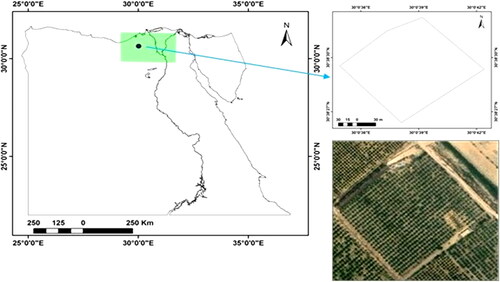
As shown in Figure 1, the study was carried out on a farm in the reclaimed land of Behera Governorate in Egypt (30°38’29.57"N, 30° 0’38.64"E). The average mean, maximum, and minimum temperatures in the study area from 1985 and 2022 were 20.7 °C, 28.4 °C, and 14.6 °C, respectively. The average wind speed was 2.9 m/s, the relative humidity averaged 59.0%, and the average daily solar radiation was 20.0 MJ/m²/day. The annual mean ETo value was approximately 4.9 mm/day. The area was arid, with an average annual precipitation of about 73 mm.

Figure 1. The study location and area.

2.2. Data acquisition

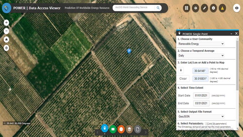
Weather data were collected from satellites and ground stations. This study used NASA’s POWER database, available on the web (https://power.larc.nasa.gov/data-access-viewer/) which is free and long-term. It provided daily global weather data on a 1° latitude-longitude grid. The data was combined from various sources, including satellites, ground observations, and modeling (White et al., 2008). Figure 2 illustrates the user interface for gathering numerous meteorology parameters including humidity, temperature, wind, and solar radiation (Brahma & Wadhvani, 2020; Torrizo et al., 2019). For this study, the daily weather data was used to estimate daily ETo for the target location using ETCalc, an online evapotranspiration calculator (Danielescu, 2022).

Figure 2. NASA’s POWER Data Access Viewer.

The weather data was collected for 38 years (1985–2022), including daily precipitation, temperature, humidity, solar radiation, and wind speed. This data was used to calculate daily evapotranspiration (ETo) using the Penman-Montieth, Hargreaves, and Blaney-Criddle methods (Schomberg et al., 2023; Tabari, 2010).

2.3. Calculation of reference evapotranspiration

This section outlines the calculation methods for ETo, including FAO-Penman-Monteith, Hargreaves, and Blaney-Criddle equations.

2.3.1. The FAO-Penman-Monteith (FAO-PM) equation

The FAO-PM is the standard equation for determining ETo. As per reference (Allen et al., 1998), it is presented in Equation (1)(1) $$\mathit{\text{ETo}}=\frac{0.408\Delta \left(Rn-G\right)+\gamma \frac{900}{T+273}\left[\mathit{\text{es}}-\mathit{\text{ea}}\right]u2}{\Delta +\gamma \ast (1+0.34\ast u2\text{)}}$$(1) : (1) $$\mathit{\text{ETo}}=\frac{0.408\Delta \left(Rn-G\right)+\gamma \frac{900}{T+273}\left[\mathit{\text{es}}-\mathit{\text{ea}}\right]u2}{\Delta +\gamma \ast (1+0.34\ast u2\text{)}}$$(1)

The reference crop evapotranspiration (ETo) is calculated using the Penman-Monteith equation, which considers the net radiation (Rn), soil heat flux (G), mean daily air temperature at 2 m (T), wind speed at 2 m (u2), saturation vapor pressure (es), actual vapor pressure (ea), vapor pressure deficit (es - ea), slope of the saturation vapor pressure-temperature curve (Δ), and psychrometric constant (γ).

2.3.2. Hargreaves equation (ETo_HA)

The Hargreaves model is a widely used version of an older evapotranspiration model (Tabari, 2010). The model’s form, as per reference (Hargreaves & Allen, 2003) is given as Equation (2)(2) $$\mathbf{\text{ETo}}=\mathbf{0.0023}\mathbf{R}\mathbf{a}\left(\mathbf{\text{Ta}}+\mathbf{17.8}\right){\left(\mathbf{\text{Tmax}}-\mathbf{\text{Tmin}}\right)}^{\mathbf{0.5}}$$(2) : (2) $$\mathbf{\text{ETo}}=\mathbf{0.0023}\mathbf{R}\mathbf{a}\left(\mathbf{\text{Ta}}+\mathbf{17.8}\right){\left(\mathbf{\text{Tmax}}-\mathbf{\text{Tmin}}\right)}^{\mathbf{0.5}}$$(2)

Ra, the water equivalent of extraterrestrial radiation, depends on the mean air temperature (Ta), daily maximum temperature (Tmax), and daily minimum temperature (Tmin).

2.3.3. Blaney-Criddle equation (ETo_BC)

The BC equation, based on the reference (Blaney & Criddle, 1962), is represented by Equation (3)(3) $$\mathbf{\text{ETo}}=\mathbf{P}\left(\mathbf{0.46}\mathbf{T}+\mathbf{8.13}\right)$$(3) , which calculates ETo as: (3) $$\mathbf{\text{ETo}}=\mathbf{P}\left(\mathbf{0.46}\mathbf{T}+\mathbf{8.13}\right)$$(3)

P and T represent the average daily percentage of total annual daytime hours and the average daily air temperature (°C), respectively.

2.4. Trend analysis of time-series data

Hydro-meteorological data from agro-climatic zones was used to identify trends in ETo and other climate variables. Nonparametric tests, such as the Mann-Kendall test, are commonly used to detect specific types of trends in meteorological time series data (Mann, 1945; Ramachandra et al., 2022).

2.4.1. Modified Mann–Kendall (m-MK) test

The Mann-Kendall test is a statistical method for detecting trends in time series data. It focuses on determining whether there is a monotonic trend, such as an increase or decrease, over the observed period, rather than estimating the magnitude of the trend (Lornezhad et al., 2023; Yao et al., 2023). The test procedure has the following steps:

1. Consider a sequence of data samples (x1, x2, …, xn) measured over time.

2. The null hypothesis (H0) states that the data points are random and do not show a trend.

3. The alternative hypothesis (H1) suggests that there is a monotonic trend during the period.

4. The Mann-Kendall test statistic, denoted as S, is calculated using the following equation:

(4) $$S={\displaystyle \sum _{k=1}^{n-1}{\displaystyle \sum _{j=k+1}^n\mathit{\text{sgn}}\left(\mathit{\text{xj}}-\mathit{\text{xk}}\right)}}$$(4) where xi and xj represent the data points in the data set (with 1 < i < j < n), and n denotes the size of the data set. The sign function (sgn()) is the same as the sign of its argument: 1 if the argument is positive, 0 if the argument is zero, and -1 if the argument is negative. (5) $$\mathit{\text{sgn}}\left(\mathit{\text{xj}}-\mathit{\text{xk}}\right)=\left\{\begin{array}{c}1\text{\hspace{0.17em}\hspace{0.33em}if\hspace{0.33em}\hspace{0.17em}(xj\hspace{0.17em}}‐\text{xk)\hspace{0.17em}}\text{>}\hspace{0.17em}0\hspace{0.17em}\\ \hspace{0.17em}0\text{\hspace{0.33em}\hspace{0.17em}if\hspace{0.33em}\hspace{0.17em}(xj\hspace{0.17em}}‐\text{xk)\hspace{0.17em}}\text{=}\hspace{0.17em}0\hspace{0.17em}\\ ‐1\text{\hspace{0.17em}\hspace{0.33em}if\hspace{0.33em}\hspace{0.17em}(xj\hspace{0.17em}}‐\text{xk)\hspace{0.17em}}\text{<}\hspace{0.17em}0\hspace{0.17em}\end{array}\right.$$(5)

In the modified Mann-Kendall (m-MK) tests (Hamed & Rao, 1998; Sa’adi et al., 2019), the equivalent normal variants of the rank for the de-trended series are calculated using the following equation: (6) $$\text{Zi}=\Phi -\text{1\hspace{0.17em}}\left(\frac{\mathit{\text{Ri}}}{n+1}\right)f\text{\hspace{0.33em}}\mathit{\text{or}}i\hspace{0.17em}=1:n$$(6) where Ri is the rank of the de-trended series xj, n is the length of the time series, and $\Phi -1$ is the inverse standard normal distribution function (mean = 0, standard deviation = 1).

2.4.2. Theil–Sen’s estimator

The Mann-Kendall test is useful for detecting monotonic trends, it cannot estimate their slope. Sen’s slope is a nonparametric method that is commonly used to estimate the magnitude of trends in a sample of n data pairs (Ramachandra et al., 2022). It is robust to missing values, outliers, and non-normality (Sen, 1968).

The slope of the data trend was estimated using Sen’s method as:The slope for each pair of data points was calculated and then

1. the middle value of all the slopes calculated in step 1 was found.

The slope of n pairs of data points was estimated using the equation: (7) $$\beta =\mathit{\text{Median}}\left(\frac{\mathit{\text{Xj}}-\mathit{\text{Xi}}}{j-i}\right)\mathit{\text{for}}\text{\hspace{0.33em}}\mathit{\text{all}}i<j$$(7)

Here, 1 < j < i < n, and β represent the estimate of the trend magnitude. A positive value of β indicates an upward trend, while a negative value of β suggests a downward trend.

2.5. Dataset pre‑processing: handling missing values, outliers, and normalization

The forecasting models are biased by missing data, so to solve this problem, imputation techniques such as mean or median imputation can be used to estimate and replace missing data (Khan & Hoque, 2020). Outliers in datasets can skew the analysis. These were detected and handled using methods including Z-score and IQR (Singh & Haider, 2022). Normalization of the data in the ML pre-processing was used to bring different features with a similar range, reducing bias and improving the model’s learning effectiveness.

Min-max normalization was used to normalize the training and test examples to the range between 0 and 1 using Equation (Soomro et al., 2022): (8) $$X^{\mathit{\text{norm}}}=\frac{X^n\hspace{0.17em}-X^{\text{min}}}{X^{\text{max}}-X^{\text{min}}}$$(8) where X_norm is the normalized value, Xn is the original value, X_max is the maximum value, and X_min is the minimum value.

2.6. Machine learning models for predicting reference evapotranspiration (ETo)

In this study, six regression models were used, described below, to predict ETo and compared their performance to the three well-accepted models described above using conventional statistical evaluation indicators. To evaluate the model’s performance, the dataset was split into training and testing sets in an 80:20 ratio (Gul et al., 2023). The training dataset included essential input variables for BC, HA, and PM. BC utilized mean air temperature, HA involved minimum, maximum, and mean air temperature, while PM considered minimum, maximum, mean air temperature, wind speed, relative humidity, and solar radiation. The common output variable for all methods was ETo.

2.6.1. Simple linear regression (SLR) and multiple linear regression (MLR)

Linear regression is a prevalent statistical and machine learning algorithm employed to establish relationships between predictors, facilitating pattern identification and data-based predictions. Simple linear regression (SLR) predicts evapotranspiration (ETo) using one independent variable. So, it was used with the Blaney-Criddle method. Conversely, multiple regression (MLR) incorporates multiple variables to predict ETo, calculated using both the Penman-Montith and Hargreaves equations (Maulud & Abdulazeez, 2020).

2.6.2. K-Nearest Neighbours (KNN) regression

K-Nearest Neighbor (KNN) is a widely used non-parametric machine learning algorithm for classification and regression tasks. In regression, KNN calculates the object’s value by averaging the values of its K closest neighbors. KNN is known for its simplicity, fast implementation, and lack of training period compared to other algorithms (Azzam et al., 2022). In this study, the significant hyperparameter utilized in KNN was the number of neighbors.

2.6.3. XGboost

XGBoost is an ensemble learning algorithm that combines multiple weak learners to improve prediction accuracy (Chen & Guestrin, 2016) .It uses gradient boosting to build a tree ensemble, and can be parallelized for faster computation (Wu & Fan, 2019). XGBoost is a popular choice for machine learning tasks due to its ability to handle overfitting and its good performance (Shi et al., 2019).

2.6.4. Support vector regression (SVR)

SVR was sophisticated by (Sain, 1996). SVR accurately splits training data and solves the widest separation hyperplane (Xie et al., 2021). Data normalization and standardization are crucial preprocessing steps for SVR. SVR aims to minimize the error between predicted and actual values by finding the optimal hyperplane during training. It identifies support vectors and, if needed, inserts a margin around the boundary for more flexible modeling of non-linear decision boundaries using kernel-induced feature spaces (Thongkao et al., 2022). The kernel (rbf), C (cost), epsilon, and gamma—which are the four crucial hyperparameters in SVR - were employed in this study.

2.6.5. Decision tree

Decision Tree (DT) is commonly used for supervised learning in classification and regression tasks. It consists of leaf nodes, paths, decision nodes, and edges, visualized as a flowchart-like tree. Core nodes signify attribute tests, branches show test results, and leaf nodes represent classes as noted by (van der Aalst, 2001). In this model, the three significant hyperparameters, including the minimum sample split, maximum depth of the tree, and minimum samples at a leaf node, were used.

2.6.6. Random forest

The Random Forest (RF) is a modification of decision trees. It was first introduced by (Breiman, 2001). RF is a group of methods for data classification and regression. Overfitting is not a concern due to the Strong Law of Large Numbers, which ensures the stability of the RF model (dos Santos Farias et al., 2020). Four critical hyperparameters were utilized in this model: the number of trees in the forest, tree depth, the minimum sample split, and the number of samples at a leaf node.

2.7. Tuning hyper-parameters

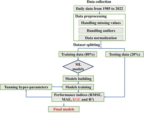
Hyperparameter adjustment is crucial for controlling ML model behavior. This process includes specifying the model, defining hyperparameter ranges, selecting a method for sampling values, establishing evaluation criteria, and choosing a cross-validation technique. Hyperparameter tuning is a pivotal step in ML model development, profoundly impacting performance and predictive accuracy (Thongkao et al., 2022). GridSearchCV automates the process of hyperparameter tuning, aiding in the determination of optimal values for a given model. GridSearchCV streamlines the hyperparameter tuning process, saving time and resources compared to manual methods (Alhakeem et al., 2022). The flowchart in Figure 3 illustrates the key stages, including data preparation, model training, and other steps, in predicting ETo.

Figure 3. Flowchart of ETo prediction algorithm for the prediction of ETo.

2.8. Statistical evaluation

The performance of machine learning (ML) algorithms was evaluated using the coefficient of determination (R²), root mean square error (RMSE), mean absolute error (MAE) (Azzam et al., 2022), and the Kling–Gupta efficiency (KGE) (Rezaiy & Shabri, 2023). The KGE assesses the agreement between a model’s predicted values and the calculated data. KGE values span from –∞ to 1, with higher values indicating enhanced model performance. The KGE of 1 signifies perfect agreement between predicted and calculated data, while lower values indicate less precise model performance (Rezaiy & Shabri, 2023). The equations for these performance evaluation metrics are as follows: (9) $${\mathrm{R}}^2=1-\frac{\mathit{\text{RSS}}}{\mathit{\text{TSS}}}$$(9) (10) $$\mathit{\text{RMSE}}=\sqrt{\frac{1}{n}{{\displaystyle \sum }}_{i=1}^n{(\mathit{\text{xi}}\hspace{0.17em}-\hspace{0.17em}\mathit{\text{yi}})}^2\hspace{0.17em}}$$(10) (11) $$\mathit{\text{MAE}}=\frac{1}{n}{{\displaystyle \sum }}_{i=1}^n\text{yi\hspace{0.17em}}-\text{\hspace{0.17em}xi}$$(11) (12) $$\mathit{\text{KGE}}=1-\sqrt{{\left(r-1\right)}^2+{\left(\alpha -1\right)}^2+{\left(\beta -1\right)}^2}$$(12) 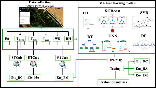x, y, RSS, and TSS represent the observed variable, the simulated variable, the sum of squares of residuals, and the total sum of squares, respectively. In the final equation, "r" denotes the Pearson correlation coefficient between predicted and calculated values, "α" represents the ratio of the standard deviation of predicted data to that of calculated data, and "β" signifies the ratio of the mean of predicted data to that of calculated data (Rezaiy & Shabri, 2023). Figure 4 depicts the various stages used in the study to assess the efficacy of several machine learning algorithms for predicting ETo values.

Figure 4. Demonstrate the methodology of the study.

3. Results and discussion

The results are given in the form of the analysis of reference evapotranspiration (ETo) and other climate variables, the prediction of daily ETo values, and the Performance analysis of ML models.

3.1. Temporal analysis of reference evapotranspiration (ETo) and other climate variables

The understanding of evapotranspiration and climate trends is vital for effective water resource management in arid and semi-arid regions (Fouad et al., 2022; Yassen et al., 2020). So, the dataset of annual ETo values and climate variables spanning the period from 1985 to 2022 was analyzed through the utilization of the modified Mann.-Kendall test and Theil Sen’s slope estimator methods. The implementation of these tests was carried out utilizing Python version 3.9.7 within the Jupyter editor. The statistical determination of trends pertaining to both ETo and the climate variables was conducted at a significant level of 5%, and the results are presented in Table 1.

Table 1. Modified Mann-Kendall test and Sen’s slope estimator results of ETo and climate variables on annual scale.

Variables	p-Value	Trend	Slope
Precipitation	0.413	No significant trend	0.001
Mean temperature	0.000	Increasing	0.021
Max temperature	0.011	Increasing	0.016
Min temperature	0.000	Increasing	0.030
Extraterrestrial solar radiation	0.605	No significant trend	0.000
Surface solar radiation	0.000	Increasing	0.088
Wind speed	0.696	No significant trend	0.000
Relative humidity	0.386	No significant trend	0.019
PM_ET0_mm	0.000	Increasing	0.012
BC_ET0_mm	0.000	Increasing	0.003
HA_ET0_mm	0.332	No significant trend	−0.001

The analysis of precipitation revealed a p-value of 0.413, indicating a lack of significant change during the study period. So, it has no significant trend, with a slope of 0.001. On the other hand, the mean temperature exhibited a significant change with a p-value of 0.000. A clear increasing trend was identified, characterized by a slope of 0.021, indicating a steady rise in mean temperature over the years. Similarly, the maximum temperature displayed a significant change, as indicated by a p-value of 0.011. The increasing trend observed, with a slope of 0.016, signifies a gradual upward shift at the maximum temperature throughout the observed period.

Furthermore, the analysis of the minimum temperature yielded a significant change with a p-value of 0.000. The trend analysis revealed a clear increasing pattern, with a slope of 0.030, indicating a consistent rise in the minimum temperature over time. In contrast, the extraterrestrial solar radiation exhibited no significant trend, having a p-value of 0.605 and a slope of 0.000. This indicates minimal deviations in solar radiation from extraterrestrial sources during the period under examination. Surface solar radiation, on the other hand, demonstrated a significant change with a p-value of 0.000. The trend analysis revealed a substantial increasing pattern, characterized by a slope of 0.088. This indicates a steady and notable increase in surface solar radiation over the years. In contrast, wind speed exhibited no significant trend, with a p-value of 0.696, and with a slope of 0.000.

Relative humidity displayed no significant trend, as evidenced by a p-value of 0.386. However, a slight upward trend was observed, with a slope of 0.019, indicating a modest increase in relative humidity over time. Analysis of PM_ET0_mm revealed a significant change with a p-value of 0.000. The trend analysis indicated a clear increasing pattern with a slope of 0.012, suggesting a consistent rise in PM_ET0_mm over the observed period. Similarly, BC_ET0_mm exhibited a significant change, as denoted by a p-value of 0.000. The trend analysis revealed a clear increasing pattern, characterized by a slope of 0.003, indicating a gradual rise in BC_ET0_mm throughout the observed period. Conversely, HA_ET0_mm displayed no significant trend, with a p-value of 0.332. The trend analysis indicated a slight decrease, as denoted by a slope of −0.001, suggesting a minor decline in HA_ET0_mm over the years.

The same finding found in the study (Fouad et al., 2022) that affirms a rising temperature trend in Egypt, with a clear positive annual temperature trend of 0.87 °C for 116 years (1901–2016). Also, this research (Yassen et al., 2020) observed noteworthy spatial distribution changes in evapotranspiration, particularly notable since the 1980s.

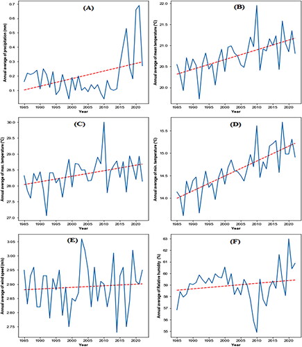
Figure 5 presents an overview of some climate data, which is crucial for sophisticated water management and decision-making. The analysis of Precipitation data showed the mean, minimum, and maximum annual averages of 0.2, 0.04, and 0.69 mm, respectively. The lowest values occurred in 1999 and 2010, while the highest value was observed in 2021. Regarding temperature, the yearly average (T mean) yielded mean, minimum, and maximum values of 20.7 °C, 19.7 °C, and 22.0 °C, respectively. The yearly average (T max) displayed mean, minimum, and maximum temperature values of 28.4 °C, 27.1 °C, and 30.0 °C, respectively. The yearly average (T min) showed mean, minimum, and maximum values of 14.6 °C, 13.6 °C, and 15.7 °C, respectively. In examining wind speed and relative humidity data, the mean values were determined to be 2.9 m/s and 59.0%, respectively. The minimum values were 2.7 m/s and 54.9%, while the maximum values were 3.1 m/s and 63.0%.

Figure 5. The long period climate values of (A) precipitation (mm), (B) mean temperature (°C), (C) maximum temperature (°C), (D) minimum temperature (°C), (E) wind speed (m/s), (F) relative humidity (%) of study area from (1985–2022).

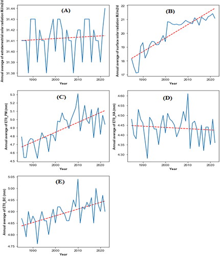
Figure 6 presents an overview of ETo, extraterrestrial and surface solar radiation. The extraterrestrial solar radiation remained stable at the mean, minimum, and maximum values of 31.4 MJ/m2/day. Surface solar radiation, however, displayed mean, minimum, and maximum values of 20, 17.1 , and 21.4 MJ/m²/day, respectively. For ETo, the mean values of ETo-PM, ETo-HA, and ETo-BC were 4.9, 4.4, and 4.9 mm/day, respectively. The minimum values were 4.5, 4.3, and 4.8 mm/day, while the maximum values were 5.3, 4.6, and 5 mm/day, respectively Bai et al. (2010) analyzed NASA/POWER data on temperature and relative humidity at 2 m height to compare with observed data from twenty weather stations in Egypt. Missing data were found in the ground weather observations. Missing data were found in the ground weather observations. Results showed a significant correlation between NASA/POWER and observed data for all parameters except RH. The study suggested the use of NASA/POWER datasets in the absence or scarcity of observations in Egypt while acknowledging the need for improvements considering the influence of the Mediterranean Sea. Other studies have demonstrated the applicability of NASA/POWER data for various applications, such as agriculture in China (Negm et al., 2017). Also (Agrawal et al., 2022) evaluated NASA/POWER suitability for estimating daily meteorological variables in Sicily, Italy. Despite the lack of climate data in Mediterranean countries, they discovered that the NASA POWER agro-climatology database provided precise daily evapotranspiration estimates. Inaccurate relative air humidity estimations were observed in coastal weather stations. Continuous monitoring and analysis of climatic variables, including ETo, temperature, precipitation, solar radiation, wind speed, and humidity, reveal a climate change pattern. Factoring these trends into water management decisions, especially for irrigation practices, is crucial for addressing environmental conditions.

Figure 6. The long period climate values of (A) Extraterrestrial solar radiation (MJ/m2/day), (B) Surface solar radiation (MJ/m2/day), (C) reference evapotranspiration calculated by Penman-Monteith method (PM) (mm), (D) reference evapotranspiration calculated by Hargreaves method (HA) (mm), (E) reference evapotranspiration calculated by Blaney-Criddle method (BC) (mm of study area from (1985–2022).

3.2. Predicted and calculated daily ETo values

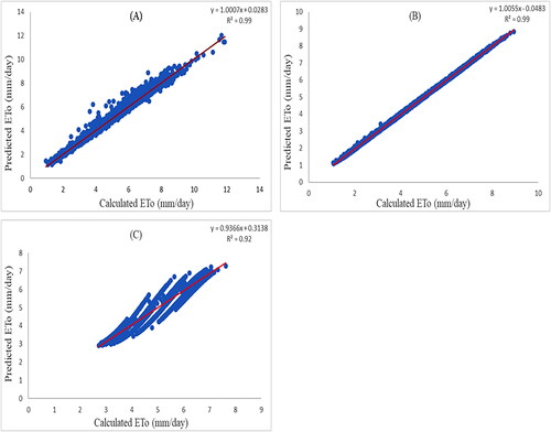
Figure 7 provides a comprehensive comparison between the calculated and predicted daily ETo values. This analysis offers a valuable assessment of the accuracy and reliability of the predictive models employed in the research. The scatter plots in Figure 7(A–C) contribute additional insights into the relationship between the predicted and calculated values. The R² values of 0.99, 0.99, and 0.92 further substantiate the strong correlation observed between the predicted and calculated ETo values. A high R² value of 0.99 indicates an exceptional level of agreement between the two sets of values, suggesting that the predictive model accurately captures the variations in the data. Although the R² value of 0.92 for BC is slightly lower, it still signifies a robust correlation between the predicted and calculated values.

Figure 7. Scatter plots showing.the comparison of predicted.and actual ETo values and their.relationship for (A) Penman-Monteith.method (PM) (mm), (B) by Hargreaves method (HA), and (C) Blaney-Criddle method (BC) during the testing period.

3.3. Performance analysis

Table 2 presents a comprehensive comparison of the predictive power of ML algorithms for estimating ETo. The algorithms were trained on a training dataset and evaluated on a separate testing dataset. Performance assessment utilized R², RMSE, MAE, and KGE metrics. For the PM method, the MLR algorithm for the PM performed well, with an R² value of 0.98 for the training and the testing dataset. The MLR algorithm shows low RMSE and MAE values (0.37 and 0.28 mm/day) and (0.38 and 0.28 mm/day) for both the training and testing datasets. Furthermore, the KNN algorithm displays low RMSE and MAE values (0.24 and 0.17 mm/day) and (0.28 and 0.19 mm/day) for both the training and testing datasets. The KNN algorithm shows a high R² value of 0.99 and 0.98 for both the training and testing datasets, respectively.

Table 2. Performance parameters for ETo methods using selected algorithms.

Methods	ML algorithms	Training				Testing
		R^2	RMSE (mm/day)	MAE (mm/day)	KGE	R^2	RMSE (mm/day)	MAE (mm/day)	KGE
PM	MLR	0.98	0.37	0.28	0.98	0.98	0.38	0.28	0.98
	KNN	0.99	0.24	0.17	0.99	0.98	0.28	0.19	0.98
	XGBoost	0.99	0.15	0.11	0.99	0.99	0.25	0.17	0.99
	SVR	0.99	0.22	0.14	0.99	0.99	0.24	0.15	0.99
	DT	0.98	0.30	0.22	0.99	0.97	0.39	0.29	0.98
	RF	0.99	0.23	0.15	0.99	0.98	0.26	0.18	0.99
HA	MLR	0.99	0.23	0.19	0.99	0.99	0.23	0.19	0.99
	KNN	0.99	0.01	0.01	0.99	0.99	0.06	0.04	0.99
	XGBoost	0.99	0.01	0.01	0.99	0.99	0.04	0.03	0.99
	SVR	0.99	0.05	0.04	0.99	0.99	0.05	0.04	0.99
	DT	0.99	0.13	0.10	0.99	0.99	0.17	0.13	0.99
	RF	0.99	0.20	0.15	0.99	0.99	0.21	0.16	0.99
BC	LR	0.92	0.35	0.29	0.94	0.92	0.35	0.30	0.94
	KNN	0.93	0.32	0.26	0.95	0.91	0.36	0.29	0.94
	XGBoost	0.93	0.33	0.27	0.95	0.92	0.35	0.29	0.94
	SVR	0.92	0.34	0.28	0.95	0.92	0.35	0.28	0.95
	DT	0.93	0.33	0.27	0.95	0.92	0.35	0.29	0.94
	RF	0.92	0.33	0.28	0.95	0.92	0.35	0.29	0.94

The XGBoost algorithm showed outstanding performance in the training dataset. The R² value is 0.99, and the RMSE and MAE values are (0.15 and 0.11 mm/day). It maintained impressive performance in the testing dataset, with an R² value of 0.99 and low RMSE and MAE values (0.25 and 0.17 mm/day) (Mokari et al., 2022) used the model XGBoost, to predict the ETo based on PM method and the model was the best among the selected ensembled machine learning models. Impressive results for the SVR method were observed in the training dataset, with an R² value of 0.99 and low RMSE and MAE values (0.22 and 0.14 mm/day, respectively). The SVR method maintained its exceptional performance in the testing dataset. The SVR algorithm achieved the lowest RMSE and MAE scores (0.24 and 0.15 mm/day), and it also exhibited remarkable predictive performance with an R² value of 0.99 (Jain & Gupta, 2022) conducted a study to assess the capabilities of various machine learning (ML) models, including support vector regression (SVR), for the estimation of daily ET0 using limited climatic data. The SVR model exhibited superior stability during testing. The model can be effectively applied to estimate ET0 in regions characterized by a mean annual temperature range of 4 °C to 20 °C and shows potential for estimating ET0 in arid regions where the average monthly maximum temperature exceeds 32 °C.

The DT algorithm also performed well, with an R² value of 0.98 for the training dataset and a slightly lower performance (0.97 for the testing dataset). The RMSE and MAE values were (0.30 and 0.22 mm/day) and (0.39 and 0.29 mm/day) for both the training and testing datasets, respectively. Among the ML algorithms, the DT algorithm displayed the highest RMSE value. The RF algorithm achieved outstanding results in the training dataset, with a high R² value of 0.99 and low RMSE and MAE values (0.23 and 0.15 mm/day). The RF algorithm maintained its exceptional performance in the testing dataset, with a high R² value of 0.98 and low RMSE and MAE values (0.26 mm/day and 0.18 mm/day) (Jain & Gupta, 2022) developed the random forest regression to predict the ETo. The grid search and random search approaches are used to turn the combination of hyperparameters. The RF performed well, with an R² of 0.98.

The KGE values point to the models’ ability to align predicted and calculated values. All algorithms exhibit high KGE values, suggesting excellent performance. The MLR, KNN, XGBoost, SVR, DT, and RF models consistently achieve KGE values close to or equal to 0.99 in both training and testing, indicating robust predictive accuracy. These results signify the effectiveness of these ML algorithms in capturing the complex relationships within the data and generating reliable predictions for ETo.

The HA method, using ML techniques, exhibited superior performance in predicting ETo from meteorological data. Specifically, the MLR algorithm consistently displayed high R² values of 0.99 for both the training and testing datasets. Furthermore, the algorithm demonstrated low RMSE and MAE values (0.23 and 0.19 mm/day) for both datasets. The KNN algorithm possessed an acceptable level of performance, with an R² value of 0.99 for both the training and the testing dataset. It has low RMSE and MAE values of (0.01 and 0.01 mm/day) for the training dataset. Also, low RMSE and MAE values of 0.06 and 0.04 mm/day for the testing dataset. The XGBoost algorithm performed the same as KNN in the training dataset and has low RMSE and MAE values (0.04 and 0.03 mm/day) for the testing datasets with R² equal 0.99.

The SVR algorithm achieves R² values of 0.99 for both the training and testing datasets. In the training dataset, the algorithm demonstrated low RMSE and MAE values of 0.05 and 0.04 mm/day, for both the training and testing datasets. The DT algorithm exhibited remarkable performance, achieving high R² values of 0.99 for both the training and testing datasets. Moreover, the algorithm demonstrated low RMSE and MAE values of 0.13 and 0.10 mm/day for the training dataset and 0.17 and 0.13 mm/day for the testing dataset. The RF algorithm exhibited exceptional performance by achieving the highest R² values of 0.99 for the training and testing dataset. Furthermore, it demonstrated low RMSE and MAE values of 0.20 and 0.15 mm/day for the training dataset and 0.21 and 0.16 mm/day for the testing dataset, respectively.

The consistently high KGE values of 0.99 across all algorithms and datasets indicate excellent performance in predicting reference evapotranspiration (ETo). This suggests that each ML algorithm, including MLR, KNN, XGBoost, SVR, DT, and RF, has demonstrated robust accuracy and reliability in capturing the complex patterns and relationships within the data. The uniformity in high KGE values implies the models’ consistency in aligning predicted values with calculated data, displaying their effectiveness in ETo prediction across different datasets.

Regarding the BC method. The LR algorithm performed well. The LR algorithm exhibited remarkable performance, achieving R² values of 0.92 for both the training and testing datasets. Moreover, the algorithm demonstrated low RMSE and MAE values of 0.35 and 0.29 mm/day for the training dataset and 0.35 and 0.30 mm/day for the testing dataset.

The results of the study revealed that the KNN algorithms showed the best R² value of 0.93 for the training dataset, along with the lowest RMSE and MAE values of 0.32 and 0.26 mm/day, respectively. Furthermore, the algorithms achieve an R² value of 0.91 for the testing dataset and the low RMSE and MAE values of 0.36 and 0.29 mm/day, respectively.

The XGBoost and DT have the same performance, with R² values of 0.93 for the training and 0.92 for the testing datasets. The RMSE and MAE values were (0.33 and 0.27 mm/day) for the training. Also, they achieved low RMSE and MAE values of 0.35 and 0.29 mm/day during the testing datasets. XGBoost achieved the values of RMSE and MAE (0.16 and 0.12 mm/day) and (0.17 and 0.12 mm/day) for the training and testing datasets, respectively.

The SVR algorithm showed its potential as an efficient tool for ETo prediction, with R² values of 0.92 for both the training and testing datasets. It achieved approximately the same RMSE and MAE values of 0.34 and 0.28 mm/day for the training and the testing dataset. The RF algorithm performed well by achieving the highest R² values of 0.92 for the training and testing dataset. Furthermore, it demonstrated low RMSE and MAE values of 0.33 and 0.28 mm/day for the training dataset and 0.35 and 0.29 mm/day for the testing dataset, respectively. The consistently high KGE values, ranging from 0.94 to 0.95, indicate powerful performance across different algorithms. This suggests that MLR, KNN, XGBoost, SVR, DT, and RF models exhibit a robust ability to predict reference evapotranspiration (ETo) with accuracy and reliability. The uniformity in high KGE values for both training and testing datasets highlights the consistency of these algorithms in aligning their predictions with calculated ETo values, affirming their effectiveness in diverse datasets.

The KGE values for ML algorithms across PM, HA, and BC methods demonstrate consistently high performance. While the PM and HA methods exhibit uniform excellence, the BC method, though slightly lower, still maintains strong predictive capabilities, reflecting the overall effectiveness of ML algorithms in ETo prediction across calculation methods. In this study (Hamed et al., 2022), the efficacy of thirty empirical ET models was assessed, aiming to aid model selection based on data availability. Additionally, the study employed the KGE metric to evaluate the models’ performance. The findings identified the temperature based Hamon model as the most effective, with the HA and PM models outperforming the BC model in terms of efficiency.

4. Conclusions

This study examined climate data trends over 38 years using the modified Mann-Kendall (m-MK) test and Theil Sen’s slope estimator methods to identify trends. The results revealed significant changes in variables like temperature, solar radiation, and evapotranspiration (ETo), indicating climate change impacts in this study area. ML algorithms performed well in predicting ETo for Penman-Monteith (PM), Hargreaves (HA), and Blaney-Criddle (BC) methods, displaying R² values from 0.91 to 0.99. The observed ETo_PM and ETo_BC increased align with climate change impacts on water resources. The study emphasized ML’s efficacy in developing accurate ETo prediction models, vital for sustainable water management. These results informed water resource policymakers and contributed to adaptive strategies for climate change impacts, facilitating improved irrigation planning and resource conservation in the study area.

Authors’ contributions

Yasser Arafa contributed in the conception and design, Mohamed A. Youssef, M. Hafez and Y. Rashad contributed in the analysis, Troy Peters contributed in the interpretation of the data investigation, Ahmed Abd-ElGawad and Y. M. Rashad contributed in the drafting of the paper, Mohammed A. El-Shirbeny and Mohamed A. Youssef contributed in revising the paper critically for intellectual content and the final revision. All authors have read and agreed to the published version of the manuscript.

Disclosure statement

The authors declare no conflict of interest.

Data availability statement

Data that support the findings of this study are available from the corresponding author upon reasonable request.

Additional information

Funding

This work was funded by King Saud University, Riyadh, Saudi Arabia through the researchers supporting project number (RSPD2024R676).

Notes on contributors

Mohamed A. Youssef

Mohamed A. Youssef (MSc) is a Teaching Assistant at Ain Shams University, his research focuses on the utilization of remote sensing data in agricultural contexts. With specialized expertise, he investigates the application of machine learning techniques to enhance smart irrigation systems. His contributions aim to advance the understanding and implementation of technology-driven solutions for sustainable agriculture.

R. Troy Peters

R. Troy Peters (PhD) is a Professor at Department of Biological Systems Engineering, Washington State University, Pullman, Washington, USA. Troy’s research work is in the Land, Air, Water Resources, and Environmental Engineering (LAWREE) emphasis area. His primary focus is on agricultural irrigation. This includes deficit irrigation, irrigation water hydraulics, irrigation scheduling and management, irrigation automation, sprinkler irrigation efficiency, low energy precision application (LEPA), low elevation spray application (LESA), and crop water use estimation.

Mohammed El-Shirbeny

Mohammed El-Shirbeny (PhD) is a Professor at National Authority for Remote Sensing and Space Sciences. I have extensive experience in the handling of remote sensing data and the application of data science techniques for agricultural water management and climate change-related aspects within the agricultural system. Also, I am developing the Stand-alone remote Sensing Approach to estimate the Reference Evapotranspiration (SARE).

Ahmed M. Abd-ElGawad

Ahmed M. Abd-ElGawad (PhD) is a Professor of Plant Ecology, College of Food and Agricultural Sciences, King Saud University, Saudi Arabia. His interest area is plant ecology, plant-plant interactions, chemical ecology, eco-physiology and phytotoxicity dynamics.

Younes M. Rashad

Younes M. Rashad (PhD) is an associate professor in Plant Protection and Biomolecular Diagnosis Department, Arid Lands Cultivation Research Institute (ALCRI), City of Scientific Research and Technological Applications (SRTA-City), New Borg, El-Arab, Egypt. His research interest include plant biotic and abiotic stresses and mycorrhizal fungi.

Mohamed Hafez

Mohamed Hafez Ph.D. Researcher of Environmental Soil Chemistry at the Department of Soil Science and Soil Ecology, Saint Petersburg State University, Russia. Researcher at Land and Water Technologies department, City of Scientific Research and Technological Applications, Egypt. Dr. Hafez serves as a reviewer for many scientific highs ranked journals. Dr. Hafez member of the Agricultural and Environmental Moscow Society, Russia. He was awarded the best publication in the international soil science conference in Moscow, 2020 and 2021 in a row. Dr. Hafez received the Distinguished Scientific Publication Award for my uncle 2020/2021 in a row. He has over 12 years of experience in research related to Environmental Soil Chemistry Studies. Finally, he has more than 30 scientific articles published in peer-reviewed journals and 6 book chapters.

Yasser Arafa

Yasser Arafa is a Professor at Ain Shams University, his expertise lies in on-farm irrigation, drainage systems engineering, and farm mechanization, with a specialized focus on smart irrigation systems. He is dedicated to advancing precision farming by integrating cutting-edge technologies into my research pursuits. Additionally, he has actively contributed as a team member to various research projects to enhance irrigation practices and agricultural sustainability for over 25 years.

References

- Agrawal, Y., Kumar, M., Ananthakrishnan, S., & Kumarapuram, G. (2022). Evapotranspiration modeling using different tree based ensembled machine learning algorithm. Water Resources Management, 36(3), 1–18. https://doi.org/10.1007/s11269-022-03067-7
- Alhakeem, Z. M., Jebur, Y. M., Henedy, S. N., Imran, H., Bernardo, L. F., & Hussein, H. M. (2022). Prediction of ecofriendly concrete compressive strength using gradient boosting regression tree combined with GridSearchCV hyperparameter-optimization techniques. Materials, 15(21), 7432. https://doi.org/10.3390/ma15217432
- Allen, R. G., Pereira, L. S., Raes, D., & Smith, M. (1998). Crop evapotranspiration-Guidelines for computing crop water requirements-FAO Irrigation and drainage paper 56. Fao, Rome, 300(9), D05109.
- Aschonitis, V. G., Papamichail, D., Demertzi, K., Colombani, N., Mastrocicco, M., Ghirardini, A., Castaldelli, G., & Fano, E.-A. (2017). High-resolution global grids of revised Priestley–Taylor and Hargreaves–Samani coefficients for assessing ASCE-standardized reference crop evapotranspiration and solar radiation. Earth System Science Data, 9(2), 615–638. https://doi.org/10.5194/essd-9-615-2017
- Azzam, A., Zhang, W., Akhtar, F., Shaheen, Z., & Elbeltagi, A. (2022). Estimation of green and blue water evapotranspiration using machine learning algorithms with limited meteorological data: A case study in Amu Darya River Basin, Central Asia. Computers and Electronics in Agriculture, 202, 107403. https://doi.org/10.1016/j.compag.2022.107403
- Bai, J., Chen, X., Dobermann, A., Yang, H., Cassman, K. G., & Zhang, F. (2010). Evaluation of NASA satellite-and model-derived weather data for simulation of maize yield potential in China. Agronomy Journal, 102(1), 9–16. https://doi.org/10.2134/agronj2009.0085
- Bashir, R. N., Khan, F. A., Khan, A. A., Tausif, M., Abbas, M. Z., Shahid, M. M. A., & Khan, N. (2023). Intelligent optimization of Reference Evapotranspiration (ETo) for precision irrigation. Journal of Computational Science, 69, 102025. https://doi.org/10.1016/j.jocs.2023.102025
- Blaney, H. F., & Criddle, W. D. (1962). Determining consumptive use and irrigation water requirements (No. 1275). US Department of Agriculture.
- Brahma, B., & Wadhvani, R. (2020). Solar irradiance forecasting based on deep learning methodologies and multi-site data. Symmetry, 12(11), 1830. https://doi.org/10.3390/sym12111830
- Breiman, L. (2001). Random forests. Machine Learning, 45(1), 5–32. https://doi.org/10.1023/A:1010933404324
- Chen, T., & Guestrin, C. (2016). Xgboost: A scalable tree boosting system. In Proceedings of the 22nd Acm Sigkdd International Conference on Knowledge Discovery and Data Mining (pp. 785–794.).
- Chen, Z., Zhu, Z., Jiang, H., & Sun, S. (2020). Estimating daily reference evapotranspiration based on limited meteorological data using deep learning and classical machine learning methods. Journal of Hydrology, 591, 125286. https://doi.org/10.1016/j.jhydrol.2020.125286
- Chouaib, E. H., Salwa, B., Saïd, K., & Abdelghani, C. (2022). Early estimation of daily reference evapotranspiration using machine learning techniques for efficient management of irrigation water. Journal of Physics: Conference Series, 2224(1), 012006. https://doi.org/10.1088/1742-6596/2224/1/012006
- Danielescu, S. (2022). SWIB: An online model to estimate daily crop water stress, irrigation needs, and soil water budget. Groundwater, 61(3), 296–300. https://doi.org/10.1111/gwat.13278
- de Sousa Lima, J. R., Antonino, A. C. D., de Souza, E. S., Hammecker, C., Montenegro, S. M. G. L., & de Oliveira Lira, C. A. B. (2013). Calibration of Hargreaves-Samani equation for estimating reference evapotranspiration in sub-humid region of Brazil. Journal of Water Resource and Protection, 5(12A), 1–5.
- Djaman, K., O’Neill, M., Diop, L., Bodian, A., Allen, S., Koudahe, K., & Lombard, K. (2019). Evaluation of the Penman-Monteith and other 34 reference evapotranspiration equations under limited data in a semiarid dry climate. Theoretical and Applied Climatology, 137(1-2), 729–743. https://doi.org/10.1007/s00704-018-2624-0
- dos Santos Farias, D. B., Althoff, D., Rodrigues, L. N., & Filgueiras, R. (2020). Performance evaluation of numerical and machine learning methods in estimating reference evapotranspiration in a Brazilian agricultural frontier. Theoretical and Applied Climatology, 142(3-4), 1481–1492. https://doi.org/10.1007/s00704-020-03380-4
- Farooque, A. A., Afzaal, H., Abbas, F., Bos, M., Maqsood, J., Wang, X., & Hussain, N. (2022). Forecasting daily evapotranspiration using artificial neural networks for sustainable irrigation scheduling. Irrigation Science, 40(1), 55–69. https://doi.org/10.1007/s00271-021-00751-1
- Ferreira, L. B., da Cunha, F. F., de Oliveira, R. A., & Fernandes Filho, E. I. (2019). Estimation of reference evapotranspiration in Brazil with limited meteorological data using ANN and SVM–A new approach. Journal of Hydrology, 572, 556–570. https://doi.org/10.1016/j.jhydrol.2019.03.028
- Fouad, E., Elnouby, M., & Saied, M. (2022). Variability and trend analysis of temperature in Egypt. Egyptian Journal of Physics, 50(1), 47–58.
- Granata, F. (2019). Evapotranspiration evaluation models based on machine learning algorithms: A comparative study. Agricultural Water Management, 217, 303–315. https://doi.org/10.1016/j.agwat.2019.03.015
- Granata, F., & Di Nunno, F. (2021). Forecasting evapotranspiration in different climates using ensembles of recurrent neural networks. Agricultural Water Management, 255, 107040. https://doi.org/10.1016/j.agwat.2021.107040
- Gul, S., Ren, J., Wang, K., & Guo, X. (2023). Estimation of reference evapotranspiration via machine learning algorithms in humid and semiarid environments in Khyber Pakhtunkhwa, Pakistan. International Journal of Environmental Science and Technology, 20(5), 5091–5108. https://doi.org/10.1007/s13762-022-04334-1
- Hafeez, M., Chatha, Z. A., Khan, A. A., Bakhsh, A., Basit, A. b. dul., & Tahira, F. (2020). Estimating reference evapotranspiration by Hargreaves and Blaney-Criddle methods in humid subtropical conditions. Current Research in Agricultural Sciences, 7(1), 15–22. https://doi.org/10.18488/journal.68.2020.71.15.22
- Hamed, M. M., Khan, N., Muhammad, M. K. I., & Shahid, S. (2022). Ranking of empirical evapotranspiration models in different climate Zones of Pakistan. Land, 11(12), 2168. https://doi.org/10.3390/land11122168
- Hamed, K. H., & Rao, A. R. (1998). A modified Mann–Kendall trend test for autocorrelated data. Journal of Hydrology, 204(1-4), 182–196. https://doi.org/10.1016/S0022-1694(97)00125-X
- Hargreaves, G. H., & Allen, R. G. (2003). History and evaluation of Hargreaves evapotranspiration equation. Journal of Irrigation and Drainage Engineering, 129(1), 53–63. https://doi.org/10.1061/(ASCE)0733-9437(2003)129:1(53)
- Hargreaves, G. H., & Samani, Z. A. (1985). Reference crop evapotranspiration from temperature. Applied Engineering in Agriculture, 1(2), 96–99.
- Heydari, M. M., Tajamoli, A., Ghoreishi, S. H., Darbe-Esfahani, M. K., & Gilasi, H. (2015). Evaluation and calibration of Blaney–Criddle equation for estimating reference evapotranspiration in semiarid and arid regions. Environmental Earth Sciences, 74(5), 4053–4063. https://doi.org/10.1007/s12665-014-3809-1
- Hu, Z., Bashir, R. N., Rehman, A. U., Iqbal, S. I., Shahid, M. M. A., & Xu, T. (2022). Machine learning based prediction of reference evapotranspiration (et 0) using IOT. IEEE Access. 10, 70526–70540. https://doi.org/10.1109/ACCESS.2022.3187528
- Jain, S. K., & Gupta, A. K. (2022). Application of random forest regression with hyper-parameters tuning to estimate reference evapotranspiration. International Journal of Advanced Computer Science and Applications, 13(5), 742–750. https://doi.org/10.14569/IJACSA.2022.0130585
- Kar, S., Purbey, V. K., Suradhaniwar, S., Korbu, L. B., Kholová, J., Durbha, S. S., Adinarayana, J., & Vadez, V. (2021). An ensemble machine learning approach for determination of the optimum sampling time for evapotranspiration assessment from high-throughput phenotyping data. Computers and Electronics in Agriculture, 182, 105992. https://doi.org/10.1016/j.compag.2021.105992
- Khan, S. I., & Hoque, A. S. M. L. (2020). SICE: An improved missing data imputation technique. Journal of Big Data, 7(1), 37. https://doi.org/10.1186/s40537-020-00313-w
- Khan, A. A., Nauman, M. A., Bashir, R. N., Jahangir, R., ALRoobaea, R., Binmahfoudh, A., Alsafyani, M., & Wechtaisong, C. (2022). Context aware evapotranspiration (ETs) for saline soils reclamation. IEEE Access. 10, 110050–110063. https://doi.org/10.1109/ACCESS.2022.3206009
- Kumar, M., Raghuwanshi, N. S., & Singh, R. (2011). Artificial neural networks approach in evapotranspiration modeling: A review. Irrigation Science, 29(1), 11–25. https://doi.org/10.1007/s00271-010-0230-8
- Lornezhad, E., Ebrahimi, H., & Rabieifar, H. R. (2023). Analysis of precipitation and drought trends by a modified Mann–Kendall method: A case study of Lorestan province, Iran. Water Supply, 23(4), 1557–1570. https://doi.org/10.2166/ws.2023.068
- Mann, H. B. (1945). Nonparametric tests against trend. Econometrica: Journal of the Econometric Society, 13(3), 245–259. https://doi.org/10.2307/1907187
- Maulud, D., & Abdulazeez, A. M. (2020). A review on linear regression comprehensive in machine learning. Journal of Applied Science and Technology Trends, 1(2), 140–147. https://doi.org/10.38094/jastt1457
- Meshram, V., Patil, K., Meshram, V., Hanchate, D., & Ramkteke, S. D. (2021). Machine learning in agriculture domain: A state-of-art survey. Artificial Intelligence in the Life Sciences, 1, 100010. https://doi.org/10.1016/j.ailsci.2021.100010
- Mobilia, M., & Longobardi, A. (2021). Prediction of potential and actual evapotranspiration fluxes using six meteorological data-based approaches for a range of climate and land cover types. ISPRS International Journal of Geo-Information, 10(3), 192. https://doi.org/10.3390/ijgi10030192
- Mokari, E., DuBois, D., Samani, Z., Mohebzadeh, H., & Djaman, K. (2022). Estimation of daily reference evapotranspiration with limited climatic data using machine learning approaches across different climate zones in New Mexico. Theoretical and Applied Climatology, 147(1-2), 575–587. https://doi.org/10.1007/s00704-021-03855-y
- Nauman, M. A., Saeed, M., Saidani, O., Javed, T., Almuqren, L., Bashir, R. N., & Jahangir, R. (2023). IoT and ensemble long-short-term-memory-based evapotranspiration forecasting for Riyadh. Sensors, 23(17), 7583. https://doi.org/10.3390/s23177583
- Ndulue, E., & Ranjan, R. S. (2021). Performance of the FAO Penman-Monteith equation under limiting conditions and fourteen reference evapotranspiration models in southern Manitoba. Theoretical and Applied Climatology, 143(3–4), 1285–1298. https://doi.org/10.1007/s00704-020-03505-9
- Negm, A., Jabro, J., & Provenzano, G. (2017). Assessing the suitability of American National Aeronautics and Space Administration (NASA) agro-climatology archive to predict daily meteorological variables and reference evapotranspiration in Sicily, Italy. Agricultural and Forest Meteorology, 244-245, 111–121. https://doi.org/10.1016/j.agrformet.2017.05.022
- Ramachandra, J. T., Veerappa, S. R. N., & Udupi, D. A. (2022). Assessment of spatiotemporal variability and trend analysis of reference crop evapotranspiration for the southern region of Peninsular India. Environmental Science and Pollution Research International, 29(28), 41953–41970. https://doi.org/10.1007/s11356-021-15958-0
- Ravindran, S. M., Bhaskaran, S. K. M., & Ambat, S. K. N. (2021). A deep neural network architecture to model reference evapotranspiration using a single input meteorological parameter. Environmental Processes, 8(4), 1567–1599. https://doi.org/10.1007/s40710-021-00543-x
- Raza, A., Shoaib, M., Faiz, M. A., Baig, F., Khan, M. M., Ullah, M. K., & Zubair, M. (2020). Comparative assessment of reference evapotranspiration estimation using conventional method and machine learning algorithms in four climatic regions. Pure and Applied Geophysics, 177(9), 4479–4508. https://doi.org/10.1007/s00024-020-02473-5
- Rezaiy, R., & Shabri, A. (2023). Drought forecasting using W-ARIMA model with standardized precipitation index. Journal of Water and Climate Change, 14(9), 3345–3367. https://doi.org/10.2166/wcc.2023.431
- Sa’adi, Z., Shahid, S., Ismail, T., Chung, E. S., & Wang, X. J. (2019). Trends analysis of rainfall and rainfall extremes in Sarawak, Malaysia using modified Mann–Kendall test. Meteorology and Atmospheric Physics, 131(3), 263–277. https://doi.org/10.1007/s00703-017-0564-3
- Sain, S. R. (1996). The nature of statistical learning theory.
- Schomberg, H. H., White, K. E., Thompson, A. I., Bagley, G. A., Burke, A., Garst, G., Bybee-Finley, K. A., & Mirsky, S. B. (2023). Interseeded cover crop mixtures influence soil water storage during the corn phase of corn-soybean-wheat no-till cropping systems. Agricultural Water Management, 278, 108167. https://doi.org/10.1016/j.agwat.2023.108167
- Sen, P. K. (1968). Estimates of the regression coefficient based on Kendall’s tau. Journal of the American Statistical Association, 63(324), 1379–1389. https://doi.org/10.1080/01621459.1968.10480934
- Sentelhas, P. C., Gillespie, T. J., & Santos, E. A. (2010). Evaluation of FAO Penman–Monteith and alternative methods for estimating reference evapotranspiration with missing data in Southern Ontario, Canada. Agricultural Water Management, 97(5), 635–644. https://doi.org/10.1016/j.agwat.2009.12.001
- Sharma, V., & Irmak, S. (2012). Mapping spatially interpolated precipitation, reference evapotranspiration, actual crop evapotranspiration, and net irrigation requirements in Nebraska: Part I. Precipitation and reference evapotranspiration. Transactions of the ASABE, 55(3), 907–921.
- Shi, X., Wong, Y. D., Li, M. Z. F., Palanisamy, C., & Chai, C. (2019). A feature learning approach based on XGBoost for driving assessment and risk prediction. Accident; Analysis and Prevention, 129, 170–179. https://doi.org/10.1016/j.aap.2019.05.005
- Singh, S., & Haider, M. T. U. (2022). Pre-processing of datasets with best feature selection and outlier removal techniques for a fair and robust model of software defect prediction.
- Soomro, A. A., Mokhtar, A. A., Salilew, W. M., Abdul Karim, Z. A., Abbasi, A., Lashari, N., & Jameel, S. M. (2022). Machine learning approach to predict the performance of a stratified thermal energy storage tank at a District Cooling Plant Using Sensor Data. Sensors, 22(19), 7687. https://doi.org/10.3390/s22197687
- Tabari, H. (2010). Evaluation of reference crop evapotranspiration equations in various climates. Water Resources Management, 24(10), 2311–2337. https://doi.org/10.1007/s11269-009-9553-8
- Tausif, M., Dilshad, S., Umer, Q., Iqbal, M. W., Latif, Z., Lee, C., & Bashir, R. N. (2023). Ensemble learning-based estimation of reference evapotranspiration (ETo). Internet of Things, 24, 100973. https://doi.org/10.1016/j.iot.2023.100973
- Thongkao, S., Ditthakit, P., Pinthong, S., Salaeh, N., Elkhrachy, I., Linh, N. T. T., & Pham, Q. B. (2022). Estimating FAO Blaney-Criddle b-factor using soft computing models. Atmosphere, 13(10), 1536. https://doi.org/10.3390/atmos13101536
- Torrizo, L. F., & Africa, A. D. M, De La Salle University, Manila. (2019). Next-hour electrical load forecasting using an artificial neural network: Applicability in the Philippines. International Journal of Advanced Trends in Computer Science and Engineering, 8(3), 831–835. https://doi.org/10.30534/ijatcse/2019/77832019
- van der Aalst, W. M. (2001). Exterminating the dynamic change bug: A concrete approach to support workflow change. Information Systems Frontiers, 3(3), 297–317. https://doi.org/10.1023/A:1011409408711
- Wen, X., Si, J., He, Z., Wu, J., Shao, H., & Yu, H. (2015). Support-vector-machine-based models for modeling daily reference evapotranspiration with limited climatic data in extreme arid regions. Water Resources Management, 29(9), 3195–3209. https://doi.org/10.1007/s11269-015-0990-2
- White, J. W., Hoogenboom, G., Stackhouse, P. W., Jr., & Hoell, J. M. (2008). Evaluation of NASA satellite-and assimilation model-derived long-term daily temperature data over the continental US. Agricultural and Forest Meteorology, 148(10), 1574–1584. https://doi.org/10.1016/j.agrformet.2008.05.017
- Wu, L., & Fan, J. (2019). Comparison of neuron-based, kernel-based, tree-based and curve-based machine learning models for predicting daily reference evapotranspiration. PLoS One. 14(5), e0217520. https://doi.org/10.1371/journal.pone.0217520
- Xie, W., Nie, W., Saffari, P., Robledo, L. F., Descote, P. Y., & Jian, W. (2021). Landslide hazard assessment based on Bayesian optimization–support vector machine in Nanping City, China. Natural Hazards, 109(1), 931–948. https://doi.org/10.1007/s11069-021-04862-y
- Yao, K. M. A., Kola, E., Morenikeji, W., & Filho, W. L. (2023). Time series analysis of temperature and rainfall in the Savannah region in Togo, West Africa. Water, 15(9), 1656. https://doi.org/10.3390/w15091656
- Yassen, A. N., Nam, W. H., & Hong, E. M. (2020). Impact of climate change on reference evapotranspiration in Egypt. Catena, 194, 104711. https://doi.org/10.1016/j.catena.2020.104711