Dynamical systems of self-organized segregation

Figures & data

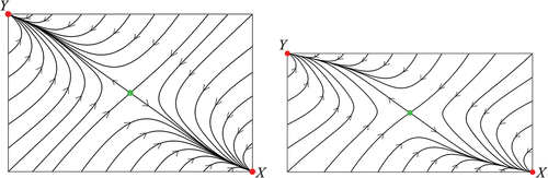
Figure 1. The dynamics of the BN model. Left: the bifurcation set consists of two surfaces separating the three open regions of parameters with the three different behaviours of the system. The smooth surface, blue, is given by (4) and the cuspy surface, green, is the discriminant set given by (9). At the red line, the dark green and light green parts of (9) meet to form a cusp. Right, bottom: the two segregated equilibria $(1,0)$ and $(0,\frac{1}{k})$, both red, attract every point except for the ones on the line separating their basins of attraction and the points on that line tend to the empty equilibrium $(0,0)$, blue. The parameter values $(\mathit{a},\mathit{b},\mathit{k})=(2,0.2,2)$ are between the smooth surface given by (4) and the two co-ordinate planes $\{\mathit{a}=0\}$ and $\{\mathit{b}=0\}$. Right, middle: a saddle, green, has detached from the origin and its stable manifold now separates the basins of attraction of the two segregated equilibria, which still attract all other points. The parameter values $(\mathit{a},\mathit{b},\mathit{k})=(2,2,2)$ are between the smooth and the cuspy surface. Right, top: there is a third attracting equilibrium, red, which is mixed. The two segregated equilibria have basins of attraction bounded by the stable manifolds of the two saddles, both green. These lines also form the boundary of the basin of attraction of the attracting mixed equilibrium. The parameter values $(\mathit{a},\mathit{b},\mathit{k})=(2,8,2)$ are in the third open region of the bifurcation set, the one bounded only by the cuspy surface given by the discriminant (9).

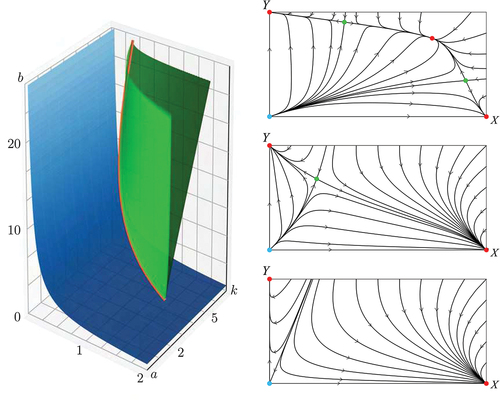
Figure 2. Left: bifurcation diagram showing saddles (green) and stable nodes (red) meeting at the fold line (blue). The surface has $0\le \mathit{X}\le 1$, ends at $\mathit{b}=1$ and we only draw it for $\mathit{k}\ge 1$. Right: for better orientation the bifurcation diagram is rotated to a top view. The saddles are no longer shown (otherwise all of $\mathit{b}\ge 1$ would be green) and the fold line forms a cusp at $(\mathit{k},\mathit{b})=(3,9)$ where it is projected along its vertical tangent.

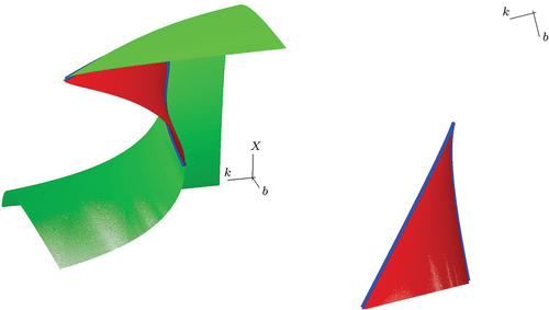
Figure 3. Phase portraits for $\mathit{a}=1$, $\mathit{k}=3.5$ and (bottom to top and left to right) $\mathit{b}=11$, $\mathit{b}=b_{-}(3.5)$, $\mathit{b}=12$, $\mathit{b}=16$, $\mathit{b}=b_{+}(3.5)$, $\mathit{b}=17$. Saddles are shown in green, stable nodes in red and non-hyperbolic equilibria in blue.

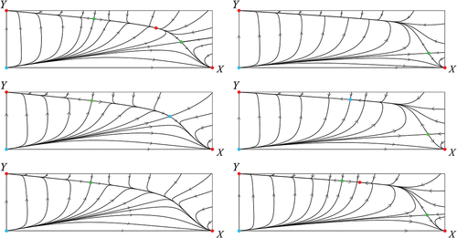
Figure 4. Bifurcation set of (16) in the $(\mathit{\alpha },\mathit{\beta })$–plane (or, equivalently, for tolerance $\mathit{a}=1$ in the $(\mathit{k},\mathit{b})$–plane). Counterclockwise (starting top right) the five pictures of nullclines have parameter values $(\mathit{\alpha },\mathit{\beta })=(2.5,6),(1.5,6),(2,4),(1.5,2),(2.5,2)$. In blue the cubic $X_1$–nullcline (dark) and the regions ${\mathcal{F}}_1^{\mathrm{i}\mathrm{n}}$, ${\mathcal{F}}_2^{\mathrm{i}\mathrm{n}}$ (light) and in red the cubic $Y_1$–nullcline (dark) and the regions ${\mathcal{G}}_1^{\mathrm{i}\mathrm{n}}$, ${\mathcal{G}}_2^{\mathrm{i}\mathrm{n}}$ (light). Where an ${\mathcal{F}}_i^{\mathrm{i}\mathrm{n}}$ and a ${\mathcal{G}}_j^{\mathrm{i}\mathrm{n}}$ intersect the colours mix to light purple. Only in the two top pictures ${\mathcal{G}}_1^{\mathrm{i}\mathrm{n}}\cap {\mathcal{G}}_2^{\mathrm{i}\mathrm{n}}\ne \mathrm{\varnothing }$ and only in the top right and bottom right pictures ${\mathcal{F}}_1^{\mathrm{i}\mathrm{n}}\cap {\mathcal{F}}_2^{\mathrm{i}\mathrm{n}}\ne \mathrm{\varnothing }$. Correspondingly, the top right picture features a (dark purple) sea of equilibria ${\mathcal{F}}_1^{\mathrm{i}\mathrm{n}}\cap {\mathcal{F}}_2^{\mathrm{i}\mathrm{n}}\cap {\mathcal{G}}_1^{\mathrm{i}\mathrm{n}}\cap {\mathcal{G}}_2^{\mathrm{i}\mathrm{n}}$. The middle left picture is also not structurally stable as small perturbations can lead to both the bottom left picture as to one of the other three pictures (the latter are clearly not structurally stable, displaying infinitely many equilibria).

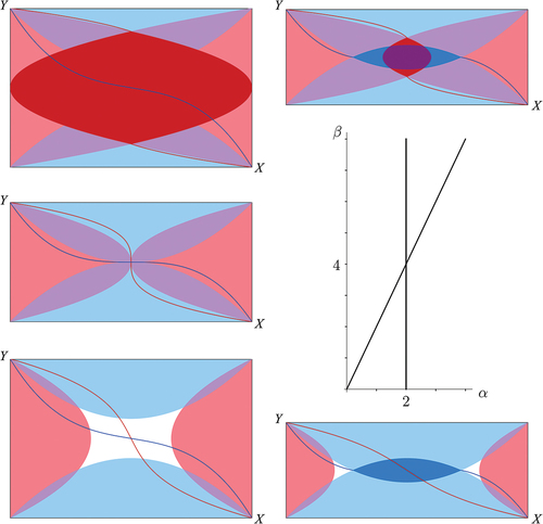
Figure 5. Phase portraits of (16) for $(\mathit{\alpha },\mathit{\beta })=(1.5,2)$, left, and for $(\mathit{\alpha },\mathit{\beta })=(2,4)$, right—the choice $\mathit{a}=1$ implies $\mathit{k}=\mathit{\alpha }$ and $\mathit{b}=\mathit{\beta }$, respectively. The left phase portrait is structurally stable while the right phase portrait is not – a fact that can be derived only by looking at small perturbations (see figure 4). Note that both phase portraits are invariant under a rotation of ${180}^{\circ }$—the dynamics of $\mathrm{B}{\mathrm{N}}_2$ coincides with that of $\mathrm{B}{\mathrm{N}}_1$.