New Zealand’s lauded fiscal legislation: has it reduced fiscal uncertainty?

Figures & data

Figure 1. Estimated government spending and net tax uncertainty – main specification.

Note: Uncertainty is the square root of the time-varying variances of structural shocks (see equation 9). The blue shaded area represents the 68 per cent credible set. The solid line is the posterior median. The pink shaded areas are recessions as identified by Hall and McDermott (2016).

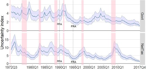
Table 2. The Pearson correlation between uncertainty estimates from alternative specifications and the uncertainty estimate from the baseline specification for the quarters 1972Q3 to 2017Q4 (unless otherwise stated).

	Govt spending uncertainty	Net Tax uncertainty
Debt included (1982Q4 to 2017Q4)	0.75	0.96
Deterministic trend model	0.95	0.98
Model with higher output/tax elasticity	0.999	0.98
Model with 90 d rate added (1985Q2 to 2017Q4)	0.91	0.98
Time Varying Parameters model (1975Q1 to 2017Q4)	0.98	0.90

Table 3. The estimated effect of the fiscal policy legislation on fiscal uncertainty: baseline model results.

	Net tax	Government spending
	(1)	(2)
During	−1.075	−0.302
	(0.889)	(0.337)
Post	−2.913***	−1.423***
	(0.641)	(0.152)
Constant	7.379***	3.659***
	(0.506)	(0.102)
Observations	182	182
R^2	0.31	0.59
F statistic (df = 2, 179)	40.4	128.4

Note: HAC standard errors reported.

Figure 2. Estimates of the percent reduction in mean uncertainty: alternative specifications and subsamples.

Note: The regression results underpinning this figure are available in Tables 1–6 of the Online Supplementary Materials. ‘Baseline’ is specification (1): the baseline model with no additional covariates; ‘US fiscal uncert’ is the baseline model with either US government or net tax uncertainty added as a covariate (see text for discussion); ‘US output uncert’ is the baseline model with US output uncertainty added as a covariate; ‘US BBD uncert’ is the baseline model with the US economic policy uncertainty of Baker et al. (2016) added as a covariate; ‘Inflation’, ‘Debt’ and ‘Output gap’ are specifications consisting of the baseline model with inflation, the government net debt-to-GDP ratio, and the output gap added as covariates respectively; ‘TVP’ is the time-varying parameters version of the baseline model; ‘Interpolated = 1’, ‘Major reform = 1’ and ‘All reform = 1’ is the baseline model with dummies for interpolated quarters, major tax reform quarters and the economic reform quarters respectively (see the text for more information); ‘1983-2017’, ‘1983-2010’ and ‘1972-2010’ are the results from the baseline model estimated on those subsamples.

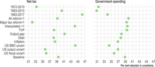
Table 1. P-values for a test of the null hypothesis of stationarity using the KPSS approach.

	log(Net tax)	log(Government spending)	log(GDP)
Trend, intercept	0.01	0.01	0.01
Intercept	0.01	0.01	0.01

Note: All three variables are real and expressed in per capital terms.

Figure 3. Response of output to a surprise doubling in fiscal uncertainty: baseline SVAR model.

Note: The shaded area represents the 68 percent credible set. The red line is posterior median. The y-axis is in percent growth rates.

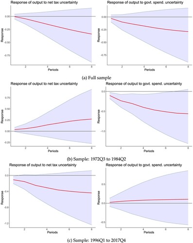
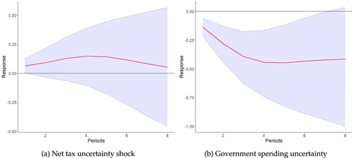
Figure 4. Response of the nominal 90 d bank bill rate to a surprise doubling in fiscal uncertainty in SVAR model with the short-term interest rate added: 1985Q2 to 2017Q4. (a) Net tax uncertainty shock. (b) Government spending uncertainty shock.

Note: The shaded area represents the 68 percent credible set. The red line is posterior median. The y-axis is in percentage points.

Hall, V., & McDermott, C. J. (2016). Recessions and recoveries in New Zealand’s post-Second World War business cycles. New Zealand Economic Papers, 50(3), 261–280. doi:10.1080/00779954.2015.1129358

 Google Scholar